Field line distribution of density at
L
=4.8 inferred from observations
by CLUSTER
R. E. Denton1, P. D´ecr´eau2, M. J. Engebretson3, F. Darrouzet4, J. L. Posch3, C. Mouikis5, L. M. Kistler5, C. A. Cattell6, K. Takahashi7, S. Sch¨afer8, and J. Goldstein9
1Department of Physics and Astronomy, Dartmouth College, Hanover, NH, USA
2Laboratoire de Physique et Chimie de l’Environnement/Centre National de Recherche Scientifique, Orl´eans, France 3Physics Department, Augsburg College, Minneapolis, USA
4Belgian Institute for Space Aeronomy, Brussels, Belgium 5University of New Hampshire, Durham, NH, USA
6Tate Physics Laboratory, University of Minnesota, Minneapolis, USA
7Applied Physics Laboratory, The Johns Hopkins University, Laurel, MD, USA
8Institut f¨ur Geophysik und extraterrestrische Physik, Technical University of Braunschweig, Germany 9Southwest Research Institute, San Antonio, USA
Received: 3 July 2008 – Revised: 3 December 2008 – Accepted: 7 January 2009 – Published: 16 February 2009
Abstract.For two events observed by the CLUSTER space-craft, the field line distribution of mass densityρwas inferred from Alfv´en wave harmonic frequencies and compared to the electron densityne from plasma wave data and the oxy-gen densitynO+ from the ion composition experiment. In
one case, the average ion massM≡ρ/ne was about 5 amu (28 October 2002), while in the other it was about 3 amu (10 September 2002). Both events occurred when the CLUSTER 1 (C1) spacecraft was in the plasmatrough. Nevertheless, the electron densityne was significantly lower for the first event (ne=8 cm−3) than for the second event (ne=22 cm−3),
and this seems to be the main difference leading to a dif-ferent value ofM. For the first event (28 October 2002), we were able to measure the Alfv´en wave frequencies for eight harmonics with unprecedented precision, so that the er-ror in the inferred mass density is probably dominated by factors other than the uncertainty in frequency (e.g., mag-netic field model and theoretical wave equation). This field line distribution (atL=4.8) was very flat for magnetic lati-tude|MLAT|.20◦ but very steeply increasing with respect to|MLAT|for |MLAT|&40◦. The total variation inρ was about four orders of magnitude, with values at large|MLAT| roughly consistent with ionospheric values. For the second event (10 September 2002), there was a small local maxi-mum in mass density near the magnetic equator. The
in-Correspondence to:R. E. Denton ([email protected])
ferred mass density decreases to a minimum 23% lower than the equatorial value at|MLAT|=15.5◦, and then steeply in-creases as one moves along the field line toward the iono-sphere. For this event we were also able to examine the spa-tial dependence of the electron density using measurements ofne from all four CLUSTER spacecraft. Our analysis in-dicates that the density varies withL atL∼5 roughly like
L−4, and thatneis also locally peaked at the magnetic equa-tor, but with a smaller peak. The value ofne reaches a den-sity minimum about 6% lower than the equatorial value at |MLAT|=12.5◦, and then increases steeply at larger values
of|MLAT|. This is to our knowledge the first evidence for a local peak in bulk electron density at the magnetic equa-tor. Our results show that magnetoseismology can be a useful technique to determine the field line distribution of the mass density for CLUSTER at perigee and that the distribution of electron density can also be inferred from measurements by multiple spacecraft.
Keywords. Magnetospheric physics (Magnetospheric con-figuration and dynamics; MHD waves and instabilities; Plas-masphere)
1 Introduction
growth and propagation of electromagnetic ion cyclotron (EMIC) waves. The field line dependence of electron den-sity affects the growth and propagation of magnetospheric whistler waves, hiss and chorus.
Direct measurement of mass density in the Earth’s magne-tosphere is difficult because it requires particle detectors with mass discrimination capable of measuring particles with low (∼eV) energies. Because of this, and also because of the po-tential for remote sensing, toroidal (azimuthally oscillating) Alfv´en wave frequencies have increasingly been used to de-termine magnetospheric mass density both from the ground (Waters et al., 2006) and from space (Denton, 2006). We sometimes refer to this as magnetoseismology.
Assuming a power law form for the mass density, a num-ber of authors have used toroidal Alfv´en wave harmonic fre-quencies to infer the field line dependence of mass density (see references in Denton, 2006, and Waters et al., 2006). Price et al. (1999) cast the wave equation into finite differ-ence form in order to solve for the mass density at several locations along a field line. Denton et al. (2001, 2004) solved for the field line dependence of mass density using a polyno-mial expansion in a coordinate related to distance along the field line. These last two studies revealed an equatorial peak in mass density. Statistical studies (Takahashi et al., 2004; Denton et al., 2006; Takahashi and Denton, 2007) have re-vealed that the tendency for the mass density to peak at the magnetic equator is greatest for largeL&6 in the afternoon local time sector, especially during geomagnetically active times. We defineLto be the maximum radius to any point on the field line (based on the TS05 model (Tsyganenko and Sitnov, 2005)) divided byRE. In dipole coordinates, this is the ordinaryLshell.
For this paper we return to an event study. Although the statistical studies of toroidal Alfv´en frequencies have the greatest potential for revealing the typical field line depen-dence and give some indication of the range of variability, it is not clear exactly how much of the variability in possible solutions is due to actual variation in the field line depen-dence at different times and how much is related to the un-certainty of the frequencies measured for individual events (Takahashi and Denton, 2007). (Takahashi and Denton ar-gued that both of these contribute to the range of possible solutions.) For instance, we can conclude from Takahashi and Denton’s results that forL>6 in the afternoon local time sector, there is on average a peak in mass density at the mag-netic equator, but we are not sure how much variability there is in the statistical distribution, that is, to what extent the dis-tribution can be more or less peaked. For this reason, it is still of interest to look at individual events, particularly if the fre-quencies can be measured with great accuracy. In this study, we use toroidal Alfv´en frequencies observed by the CLUS-TER spacecraft on 28 October 2002 in order to find what is probably the most precise field line distribution of mass den-sity determined to date, one for which the errors in the in-ferred mass density are probably dominated by factors other
than the uncertainty of the Alfv´en frequencies (e.g., magnetic field model and theoretical wave equation).
The best technique for determining the field line depen-dence of electron density is probably the active sounding technique of Reinisch et al. (2004), but this technique has so far been useful for detecting the near-equatorial density distribution only in the plasmasphere, where electron den-sity is relatively flat (Denton et al., 2006). Here we develop a least squares fitting technique for probing the distribution of electron density using plasma wave observations by the four CLUSTER spacecraft. For an event on 10 September 2002, we find (to our knowledge for the first time) an equa-torial peak in bulk electron density at the same time that we find a (larger) equatorial peak in mass density inferred from Alfv´en wave frequencies. In Sect. 2, we describe our method for inferring mass density; in Sect. 3, we describe our least squares fitting method for determining the spatial distribu-tion of electron density; in Sect. 4, we describe our results for the field line distribution of the mass density on 28 Octo-ber 2002; in Sect. 5, we describe our results for the field line distribution of mass and electron density for 10 September 2002; in Sect. 6, we compare the densities to other density measurements and compare the two events to each other; and in Sect. 7, we end with discussion.
2 Solving for the mass density
Our method for solving for the mass densityρis described by Denton et al. (2004). In brief, we solve the Alfv´en wave equation (Singer et al., 1981) with perfectly conducting ionospheric boundaries using the TS05 magnetic field model (Tsyganenko and Sitnov, 2005) and the following form for the base 10 logarithm of the mass densityρ
log10ρ=c0+c2τ2+c4τ4+c6τ6+. . . , (1)
with up to seven terms (up toc12τ12). The Alfv´en crossing time coordinateτ is
τ ≡
Z ds
VA
, (2)
a field line dependence forρ for the purpose of definingτ. Here, we use a power law field line distribution,
ρ=ρ0
LR E
R
α
, (3)
whereRis the geocentric radius, andLREis the largest value of R at any point on the field line (normally the magnetic equator); at the location corresponding to this largest value of
R, the mass density isρ0. The power law coefficient is found from the slope of the observed frequencies as described by Denton and Gallagher (2000). Please note carefully that the power law form here is used only to define the coordinate
τ used by our method. The resulting field line distribution using Eq. (1) is not restricted to the form of Eq. (3).
To find the coefficientsci yielding theoretical frequencies
fth−n best matching the observed frequencies fobs−n, we
minimize
σ ≡
v u u t 1
Nfreq
Nfreq X
n=1
f
th−n
fobs−n − 1
2
, (4)
wheren is the harmonic number (number of antinodes be-tween the ionospheric boundaries for the electric field or ve-locity perturbation) andNfreqis the number of harmonics
ob-served. We first do a grid search over a range of values for the coefficientsci, and then use a root finding or minimiza-tion routine to zero in on the soluminimiza-tion (Press et al., 1997).
Alternately we may solve for the density using
log10ρ=C0+C2z2+C4z4+C6z6+. . . , (5)
wherez=√1−R/(LRE), whereRis the geocentric radius, andLRE is defined as the maximum distance to any point along the field line. In dipole coordinates, L is the usual
L shell, and z is the sine of the dipole coordinate latitude MLAT. (It was not possible to use the coordinate τ′ used by Takahashi and Denton (2007) because the usefulness of that coordinate requires that the mass density not have a large variation along the field line, and we found that there was a large variation, especially for the event observed on 28 October 2002.) For the solution of the wave equation, we assume a perfectly conducting boundary at a height of 300 km (120 km) for the 28 October 2002 (10 September 2002) event. (There is no good reason for using different val-ues, but the difference in results is so small that it’s not worth redoing the calculations to make these values the same. For the 28 October 2002 event, using the 300 km height leads to values ofρthat are 0.9% higher at the magnetic equator, and 14% higher at a height of 300 km. See the discussion by Denton, 2006.)
0 1 2 3 4 5
−4 −3 −2 −1
0 +0.30
-0.01
-0.26 +0.01
( )
EZ R
( )
EX R
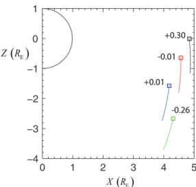
Fig. 1. CLUSTER spacecraft (where C1, C2, C3, and C4 are black, red, green, and blue, respectively) in a meridian with X=Rcos(MLAT)andZ=Rsin(MLAT). The dotted tracks show the spacecraft orbits from 11:40 UT to 12:07 UT on 10 September 2002, and the position of the spacecraft at 12:07 UT is indicated by the squares. The displacement in the out of plane (azimuthal) direc-tion at 12:07 UT is indicated by the numerals next to the squares.
3 Method for detecting the distribution of electron den-sity using multiple spacecraft
We then developed the following least squares fitting method to examine the distribution of electron density for the 10 September 2002 event. If several CLUSTER space-craft pass through a region and we are able to determine the local electron densityne along the trajectories (this method could be used with any number of spacecraft, but several are needed to constrain the possible solutions), we are able to de-termine the spatial and temporal distribution ofneunder the key assumptions of separability and smoothness. We assume that we can separate the dependence ofneinto a product of terms
ne,mod= ne,L
ne,k
ne,MLT ne,UT, (6)
wherene,Lis a function only ofL,ne,MLTis a function only
of MLT,ne,kis a function only of a parallel coordinate
(ide-ally orthogonal toLand MLT), andne,UTis a function only
of the time in hours. In addition, we assume that these sep-arated dependencies are relatively smooth (first few deriva-tives continuous) so that we can describe them in terms of a superposition of a few simple functions (like polynomials).
The problem becomes easier to solve numerically if we take the (natural) logarithm of Eq. (6),
ln ne,mod=ln ne,L+ln ne,k
+ln ne,MLT+ln ne,UT. (7)
Now suppose that we can write the individual logarithmic dependencies in terms of a sum of terms depending on the coordinate. For instance, for theLdependence, we may use
ln ne,L=aL,0+aL,1 ln(5/Ld), (8)
whereLdis theLvalue based on a dipole field, that is, Ld=
R
cos(MLAT′)2. (9)
whereRis the geocentric radius, MLAT′(defined in Eq. 11)
has values very close to those of the magnetic latitude MLAT, and the number “5” in Eq. (8) is an arbitrary choice. With (8),
ne,Lis exp ln ne,L, or
ne,L=exp aL,0
5
Ld
aL,1
, (10)
showing that this is a power law dependence in terms ofLd. The adjusted magnetic latitude MLAT′is
MLAT′≡MLAT−MLAT0. (11)
Using the TS05 magnetic field model to map the position of the CLUSTER spacecraft to the position of maximum geocentric radius, we find that this position is offset from MLAT=0 by MLAT0 (1.63◦ for the 10 September 2002
event), and we judge MLAT=MLAT0to be a better
descrip-tion of the locadescrip-tion of the magnetic equator. Note that the measured values ofneobserved by the CLUSTER spacecraft
for the 10 September 2002 event peaked at this slightly offset value.
Alternately, we may use a more general polynomial ex-pansion,
ln ne,L=aL,0+aL,1Ld+aL,2L2d+aL,3L3d, (12)
where in most cases we drop the last (cubic) term. Keep in mind that theaterms are constants that multiply field values (e.g.,Ld). With Eq. (12),ne,Lis
ne,L=exp
aL,0+aL,1Ld+aL,2L2d+aL,3L3d
. (13)
For the parallel dependence (along the field lines), we use either
ln ne,k=ak,1ln(Ld/R) , (14)
or
ln ne,k=ak,1z′+ak,2z′2+ak,3z′3+ak,4z′4 +ak,5z′
5
+ak,6z′ 6
, (15)
where only a limited number of these terms is typically kept. Equation (14) yieldsne,k=(Ld/R)aL,1, which is the power law form (3) forne(rather thanρ) withα=ak,1. For a dipole
field, (Ld/R)aL,1=1/cos2(MLAT), a function of MLAT; MLAT is not an orthogonal coordinate to Ld, and neither is MLAT′. (This is not a terrible problem, but it should be kept in mind thatLd and MLAT′ are not entirely indepen-dent.) Equation (15) is a polynomial expansion in terms of
z′, where
z′=sin MLAT′
(16) only on theLd=5 magnetic field line. At other field lines,z′ is really a function of the parallel dipole coordinate
µ= sin MLAT ′
R2 (17)
that is orthogonal toLd. Our procedure is to mapµtoz′on
theLd=5 magnetic field line (through a lookup table). At other values ofLd, we use the same mapping to determine
z′ from the localµvalue. At Ld6=5, z′(µ)is not equal to the local value of sin(MLAT′), becauseµdepends on both MLAT′ andLd. Since the dipole coordinateµ is orthogo-nal toLd (surfaces of constantµare orthogonal to surfaces of constantLd), z′(µ) is also orthogonal to Ld. (Usingz′ rather than sin MLAT′leads to a small but not crucial im-provement in the agreement between the model and observed densities. That is, one could satisfactorily use sin MLAT′ instead ofz′if he didn’t want to go to the trouble of convert-ing toz′.)
We also can add terms proportional to MLT′=MLT−MLT0
and to UT′=UT−UT0, where MLT0 is the average MLT
100
125
100
125
100
UT R
MLAT -36.63 -32.12 -27.41 -22.53 -17.49 -12.31 -7.03 -1.67 3.74 9.17 14.57 19.92 25.18 MLT 08:37 08:36 08:36 08:36 08:37 08:38 08:40 08:41 08:44 08:46 08:49 08:52 08:56 L 8.0 7.1 6.3 5.7 5.3 5.0 4.8 4.7 4.7 4.8 5.1 5.4 5.9 5.16 5.06 4.97 4.90 4.83 4.78 4.75 4.72 4.72 4.72 4.74 4.78 4.83 01:30 01:40 01:50 02:00 02:10 02:20 02:30 02:40 02:50 03:00 03:10 03:20 03:30 01:30 01:40 01:50 02:00 02:10 02:20 02:30 02:40 02:50 03:00 03:10 03:20 03:30 01:30 01:40 01:50 02:00 02:10 02:20 02:30 02:40 02:50 03:00 03:10 03:20 03:30
1 2
3 4
5 6
1
8
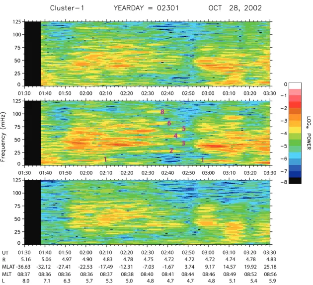
Fig. 2. Fourier spectrogram of differenced magnetic field data in field aligned coordinates for (bottom) parallel or compressional component (zˆ), (middle) azimuthal or toroidal component (yˆ∝Rˆ×ˆz), and (top) radial or poloidal component (xˆ=yˆ×ˆz). In the second panel, magenta numerals indicate the harmonic number withn=1 for the fundamental,n=2 for the second harmonic, etc.
of the event. In a number of cases, we use a term proportional to
MLT′′=MLT′−UT′. (18)
This combination takes into account corotation (for constant MLT′′, MLT′ and UT′increase together) and leads to a bet-ter match between the observations and the model than does MLT alone if explicit UT dependence is not modeled.
A full list of the possible terms used in the method appears in the middle range (between the second and third horizontal lines) of the first column of Table 1. (The specific fits will be discussed in Sect. 3.) In schematic form, we have a string of observations ofne,ne(j ), wherej is a single subscript rep-resenting the variation in time and spacecraft, and we want to approximate the values of ln(ne(j ))by
ln ne,mod(j )=
X
k
a(k) t (j, k), (19)
where the indexkrepresents one of the termst (j, k)used in the model (one of the terms listed in Table 1). The coeffi-cientsa(k)are determined to minimize the averaged squared difference between the observed values, ln(ne(j )), and the model values, ln ne,mod(j ). Since the model values come from a linear superposition, this (linear algebra) problem has a unique answer, and the standard difference
χ=
v u u t
X
j
ln ne,mod(j )
−ln(ne(j ))2
!
/Nj (20)
Table 1.Fit coefficients for ln(ne)for 10 Septtember 2002 event.
Fit
Term 1 2 3 4 5 6
1 2.90 9.85 13.1 10.1 9.99 10.0
ln(5/Ld) 4.21 – – – – –
Ld – −1.96 −3.78 −2.06 −2.05 −2.06
L2d – 0.120 0.453 0.127 0.129 0.129
L3d – – −0.0200 – – –
ln(Ld/R) 1.81 – – - – –
z′ – – – 0.143 – 0.0311
z′2 – −3.38 −2.08 −2.72 −2.73 −2.68
z′3 – – – 0.706 – −0.137
z′4 – 31.3 9.37 32.4 29.8 29.6
z′6 – – 83.8 – – –
MLT′′≡MLT′−UT′(h) −0.0114 −0.114 −0.118 −0.0931 – –
MLT′≡MLT−11.3 (h) – – – – 0.124 0.106
UT′≡UT−12.1 (h) – – – – 0.114 0.110
χ 0.0845 0.0504 0.0490 0.0451 0.0431 0.0430
exp(χ ) 1.088 1.052 1.050 1.046 1.044 1.044
close to unity, then exp(χ )−1 is the fractional error. Bothχ
and exp(χ )are listed at the bottom of Table 4.
4 Field line distribution of mass density for the 28 Oc-tober 2002 event
4.1 Alfv´en wave frequencies for 28 October 2002
Survey plots of power spectra of 4 s resolution magnetic field data from the CLUSTER Flux Gate Magnetometer (FGM) (Balogh et al., 2001) were scanned to look for toroidal Alfv´en wave events. Clear events with dominant toroidal (az-imuthal) polarization and with harmonics were not common, but there were a few. A Fourier spectrogram for one of these events observed by CLUSTER spacecraft 1 (C1) on 28 Oc-tober 2001, is shown in Fig. 2.
In order to detect toroidal Alfv´en frequencies with suf-ficient accuracy, it is necessary to take a Fourier transform over a sufficiently long time at nearly constantLshell. For a spacecraft like CRRES, the best opportunity for determina-tions of mass density based on Alfv´en frequencies is at craft apogee (Denton et al., 2004). For the CLUSTER space-craft, the orbit apogee is at geocentric radiusR∼20RE (Es-coubet et al., 2001). At this distance, magnetic field models are not reliable. Probably the best location for magnetoseis-mology using CLUSTER data is at spacecraft perigee with
R∼4–5RE. On 28 October 2001, perigee occurred at about 02:50 UT, at which time the C1 spacecraft was 3.7◦north of the SM magnetic equator at magnetic local time MLT=8.7 (dawn). The middle panel of Fig. 2 shows the power spec-trum of the toroidal (azimuthal) component of the magnetic
field and bands of wave power are clearly evident at around 02:40–02:45 UT for the second harmonic (n=2 at 27 mHz marked by the magenta label “2”) and 4th harmonic (n=4 at 55 mHz). The spacecraft crossed the SM magnetic equator at 02:43 UT, which is about the time with the clearest Alfv´en wave bands. At earlier and later times (02:00 and 03:05 UT), wave power can be seen at the fundamental frequency (n=1 at 11 mHz). Weaker but still evident at 02:43 UT are other wave bands such as the 3rd harmonic (41 mHz), 5th har-monic (67 mHz), 6th harhar-monic (80 mHz), and even the 8th harmonic (103 mHz). The harmonic indexnis the number of anti-nodes in the electric field or velocity perturbation be-tween the ionospheric boundaries. Modes with odd harmonic numbern, the fundamental, 3rd harmonic, 5th harmonic, etc. have a node (antinode) in the wave magnetic field (electric field) at the magnetic equator, while modes with evenn, the 2nd harmonic, 4th harmonic, etc. have an antinode (node) in the wave magnetic field (electric field) (Denton et al., 2004). Because of this, the 2nd harmonic and 4th harmonic are the strongest modes seen near the magnetic equator.
Fig. 3. Plot of power spectrum of the azimuthal component of the magnetic field with red diamonds at the position of mouse clicks and red lines showing the computer generated fits to the wave bands.
Then the program finds the best linear fit to the power spec-trum in the vicinity of the mouse clicks (red lines in Fig. 3). This is done by computing the integrated wave power (in-tegrated with respect to time and frequency) around the fit weighting the power at each frequency in the power spectrum by a Gaussian in the difference between the wave frequency and the fit frequency with a Gaussian width of 5 mHz.
Figure 4 is like Fig. 3, except for the power spectrum of the radial component of the electric field from the Electric-Field and Wave experiment (EFW) on Cluster spacecraft 1 (Gustafsson et al., 1997). The resolution of the data is the same as for the FGM instrument, and the power spectrum is calculated exactly the same way. In the case of the elec-tric field, the strongest waves are observed for the funda-mental and 3rd harmonic (because these harmonics have an anti-node in the electric field at the magnetic equator). The fit lines in Figs. 3 and 4 have a similar slope, and we nor-malized the frequencies to the second harmonic frequency to reduce the effect of changing frequency. These normalized frequency ratios(fn/f2)are listed in Table 2 as a function of
the harmonic numbern(=1 for the fundamental) for the mag-netic field data ((fn/f2)B) and electric field data ((fn/f2)E),
where the uncertainties are found from the variation of the frequency ratio(fn/f2)from the fit curves over the common
frequency range that was fit for bothfnandf2.
In the past, we have found the uncertainties of observed frequencies by finding the width of the frequency peaks (Denton et al., 2001, 2004, 2006; Takahashi et al., 2004). However, this method probably overestimates the error be-cause the error in the mean of a distribution is less than the width of the distribution (Takahashi and Denton, 2007). Un-fortunately, our method of estimating the error listed in Ta-ble 2 (error from range of variation in the values offn/f2
from the linear fits) yields uncertainties that are too low. We can see this by comparing the values of (fn/f2)B and
(fn/f2)E. For modesn=3, 4, and 5, the difference in these
Fig. 4. Like Fig. 3, but using the power spectrum of the radial component of the electric field.
values is 0.015, 0.023, and 0.038. These values are larger than the uncertainties listed in Table 2. However, they are smaller than the uncertainties that would result from the fre-quency resolution of the 20 min time window used for the Fourier analysis (0.8 mHz). If the uncertainty of each har-monic frequency is assumed to be the same value 1f, the uncertainty of(fn/f2),1(fn/f2)would be
1
f n
f2
=
f n
f2
s1f
fn 2
+ 1f
f2
2
= 1f
f2
s
1+ f
n
f2
2
. (21)
With 1f=0.8 mHz, or 1f/f2=0.031 (using f2=26.63 mHz), Eq. (21) yields 1(fn/f2)=0.057, 0.071,
and 0.084 for n=3–5, which is larger than the difference between(fn/f2)B and(fn/f2)E (0.015, 0.023, and 0.038). If we take 1f/f2=0.014, we get1(fn/f2)=0.026, 0.032,
and 0.038 forn=3–5, all of which are at least as great as
(fn/f2)B−(fn/f2)E (0.015, 0.023, and 0.038). The uncer-tainties in Table 2 for(fn/f2)are found using1f/f2=0.014, using Eq. (21), but the values of1(fn/f2)forn=3–5 have been reduced by a factor of 1/√2 to account for the fact that these values come from two measurements ((fn/f2)B and(fn/f2)E). The unnormalized frequencies are labelled
fn−input(mHz) in the next to last column of Table 2. These
are found by multiplying(fn/f2)byf2=26.63 mHz.
4.2 Inferred mass density for 28 October 2002
Table 2.Frequencies of toroidal harmonics for 28 October 2002 event.
n (fn/f2)B (fn/f2)E (fn/f2) fn−input(mHz) fn−solution(mHz)
1 0.410±0.003 0.410±0.015 10.92±0.40 10.95±0.42
2 1 1 1 26.63 26.63
3 1.549±0.013 1.564±0.019 1.556±0.018 41.44±0.48 41.32±0.32 4 2.038±0.005 2.061±0.006 2.050±0.022 54.59±0.59 54.63±0.37 5 2.491±0.007 2.529±0.009 2.510±0.027 66.84±0.72 67.03±0.54 6 2.999±0.001 2.999±0.044 79.86±1.2 79.23±0.84 7 3.388±0.012 3.388±0.049 90.22±1.3 90.66±0.95 8 3.883±0.010 3.883±0.056 103.4±1.5 103.3±1.3
MLAT (˚) R R( E)
3 amu cm
⎛ ⎞ ⎜ ⎟ ⎝ ⎠
A
V
τ
(a) (b)
(c) (d)
(e) (f )
Fig. 5. (Top) Mass densityρ, (middle) Alfv´en speedVA normal-ized to unity at the magnetic equator (MLAT=0), and (bottom) the Alfv´en crossing time coordinateτversus MLAT (left) and geocen-tric radiusR(right) based on solutions forρ found from Alfv´en wave frequencies observed on 28 October 2002.
uncertainties listed forfn−input in Table 2. In other words,
we pick a random set of combinations of harmonic frequen-cies such that the distribution of the frequenfrequen-cies of each har-monic is consistent with the mean and uncertainty offn−input
for the harmonic numbern. In order to determine the range of mass density distributions consistent with the frequency uncertainties, we solve for the mass density using 51 com-binations of random frequencies. However, when using all eight frequencies as input to our mass density inversion code, and using the field line distribution (Eq. 1) with 5 polyno-mial terms (c0toc8), our code did not converge on a solution
for all combinations of the frequencies we tried. We only consider solutions valid if the theoretical frequencies found by the code are within the uncertainties of the original mea-surements from the input frequencies (which may include the random variation discussed immediately above). In fact, only 51 out of 209 frequency combinations attempted resulted in a valid solution. (We keep trying random combinations until we get 51 solutions.) The actual mean and standard devia-tion of the frequencies of the harmonics used in the Monte Carlo simulation (those frequency combinations yielding a valid solution) are listed asfn−solution in Table 2. As can
be seen from Table 2, these values are within the range of frequencies listed forfn−input, but have a somewhat smaller
standard deviation.
The resulting solutions for mass density are displayed in the top panels of Fig. 5. The bold curve is the mass den-sity based on the peak frequencies. There are three thin solid curves plotted in Fig. 5a and b. At every value of MLAT, the middle thin curve shows the mean value from the Monte Carlo simulation of random combinations of harmonic fre-quencies, while the upper and lower curves show the mean plus or minus one standard deviation. However, these four curves are so close together that it is difficult to see the vari-ation. (Fig. 5c–f are discussed in Sect. 7.3.)
the frequencies were about a factor of 10 higher (because of the lowerL=4.8 shell sampled at the perigee of CLUSTER compared toL∼7 sampled by CRRES).
Whileτ may be in some sense the ideal coordinate (see Sect. 2), it is difficult to interpret the meaning of particular polynomial coefficients. For this reason, we have also solved for the field line distribution using a 5 polynomial fit forρ
with respect to thezcoordinate. Figure 6b shows that this so-lution also lies within the range of soso-lutions from the Monte Carlo simulation using theτ coordinate. This polynomial function is
log10ρ=1.57+0.35z2+0.83z4+3.95z6+4.12z8, (22)
forρexpressed in amu/cm3.
5 Mass and electron density distributions inferred for 10 September 2002
5.1 Alfv´en wave frequencies and inferred mass density for 10 September 2002
For our second event, observed at around 12:07 UT on 10 September 2002, the Alfv´en wave data is not as complete or accurate, but this event is interesting because we have better data forneandnO+and because this event has a somewhat
different field line distribution. This event occurred when the C1 spacecraft was again at perigee (geocentric radius
R=4.8RE) at MLAT=−0.2◦and MLT=11.55 (noon). The Alfv´en frequencies are found as described for the 28 October 2002 event and the frequencies and uncertain-ties are listed in Table 3 using magnetic and electric field data from the C1 spacecraft. As was the case in the first event, the uncertainties of the frequencies listed in the sec-ond and third columns found from the measured frequency ratios were judged to be too small. Based on frequency ra-tios found from the C2 spacecraft (for which the wave spectra were of lower quality; otherwise we would have used these to help calculate the harmonic frequencies), we used an error model like that used for the first event to find the uncertain-ties of the frequency ratios listed in the next-to-last column of Table 3, and those uncertainties were used in the following calculations.
Using a three polynomial fit with respect to the square of the Alfv´en crossing coordinate τ (Eq. 2), we ran our mass density inversion code to get the field line distributions shown in Fig. 7a–d (black solid curves). There is a slight peak inρnear the magnetic equator at MLAT′=0 (MLAT′=0 is at the position where the geocentric radius is maximum and the magnetic field is minimum as described in Sect. 3). The height of this peak is only 23% (as compared to a factor of 2 in the afternoon local time sector at largeL&6 (Takahashi and Denton, 2007)). The distribution of solutions from the
MLAT (˚)
z
7
(b)
peaks
ρ
ρ
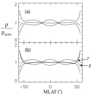
Fig. 6. (a)The (log average) mean mass densityρ(middle curve) and the meanρ plus or minus one standard deviation (upper and lower curves) at each value of MLAT based on the solutions ofρ from the Monte Carlo simulation using a 5 polynomial fit with re-spect toτ and using the eight Alfv´en wave frequencies observed on 28 October 2002. Here the values ofρare divided by the mass density found using the peak frequencies in order to better show the difference between the solutions.(b)Same curves forρplus or mi-nus one standard deviation (upper and lower curves). The middle solid (dotted) curve is the solution using the peak frequencies but with a 7 polynomial term fit with respect toτ (a 5 polynomial fit with respect toz). Both of these functions are also divided by the value ofρfound using the peak frequencies using the 5 polynomial fit with respect toτ.
Monte Carlo simulation indicated by the spread of the up-per and lower black thin solid curves in Fig. 7b does not ex-clude the possibility that the real distribution is flat. The solu-tion using three polynomial terms with respect tozis similar to that usingτ and is plotted as the black dotted curves in Fig. 7a–d. This solution is
log10ρ=1.79−1.69z2+8.38z4, (23)
forρ expressed in amu/cm3. (Fig. 7e–h will be discussed in the Discussion section.)
5.2 Spatial electron density distribution for 10 Septem-ber 2002 found from data from all four spacecraft
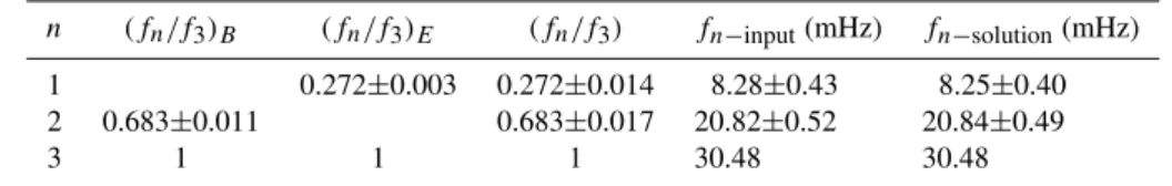
Table 3.Frequencies of toroidal harmonics for 10 September 2002 event.
n (fn/f3)B (fn/f3)E (fn/f3) fn−input(mHz) fn−solution(mHz)
1 0.272±0.003 0.272±0.014 8.28±0.43 8.25±0.40
2 0.683±0.011 0.683±0.017 20.82±0.52 20.84±0.49
3 1 1 1 30.48 30.48
in Fig. 8a but excluded the dotted portion of the green curve (C3). The reason for excluding this segment of data is that only C3 sampled the largeLdand large negative MLAT′ val-ues. The lownevalues of C3 could be modeled by alteration of either the terms describing theLdor MLAT′dependence, and which of these was affected was not well determined, leading to unnecessary variation in the solutions depending on the exact terms included in the model. Aside from C3, for which we used a start time of 12.1 UT (h), the data was used between 11.75 and 12.7 UT (times plotted in Fig. 8). These limits were chosen because of large oscillations in the C3
ne(plasma frequency) at earlier times and because C4 pene-trated into the plasmasphere at later times (not shown). How-ever, a more general treatment would allow different time limits for each spacecraft.
As described in Sect. 3, we find an optimal fit to the ob-served values of ln(ne) using a superposition of particular model functions. The models we used are listed in Table 1. For the first model, fit 1,
ne,mod 1=exp(2.90+1.81 ln(Ld/R) +4.21 ln(5/Ld)−0.0114 MLT′′ ≃18.2 cm−3
L d
R
α 5
Ld β
, (24)
(using theLshell dependence in Eq. (8) and the parallel de-pendence in Eq. 14) where we have neglected the (small) MLAT′′ dependence in the last line and the power law co-efficients for the parallel andLd directions areα=1.81 and
β=4.21. This distribution of density is extremely reason-able. Denton et al. (2004) state thatα=2–3 is typical in the plasmatrough. Values ofβ equal to 4.5 (Carpenter and An-derson, 1992), 4.0 (Sheeley et al., 2001), and 3.5 (Denton et al., 2004) have been found in statistical studies of plas-matrough density. The valueβ=4 results from the assump-tion that the flux tube content per magnetic flux is constant (Denton et al., 2004). The standard difference (of the natu-ral logarithm) isχ=0.0845, leading to a multiplicative error factor exp(χ )=1.088 (approximately a 9% error in the linear density).
In Fig. 9a, we plot the observedne values (solid curves) and model values for fit 1 (dashed curves) for all four CLUS-TER spacecraft. The model curves fit the data fairly well. We noticed, however, that the model curves in Fig. 9a have lower density than the observedneat the places where the space-craft cross MLAT′=0. These locations are indicated in Fig. 8
as vertical dashed lines for C1 (black) and C2 (red). In addi-tion, C4 reaches MLAT′=0 at the right side of the plot. Note the local increase inne at these positions. This observation led us to explore sets of model functions with a more general field line dependence. The second set of model functions for the natural logarithm ofne (fit 2 in Table 1) includes terms proportional toz′2andz′4(parallel dependence (Eq. 15)) in-stead of the power law field line dependence. (Here, sym-metry about MLAT′=z′=0 is assumed; see definitions in Sect. 3.) Fit 2 also has a quadraticLddependence (constant,
Ld, andL2d terms). For fit 2,χ=0.0504 or exp(χ )=0.0504 (roughly a 5% error), a significant improvement. The model functions for fit 2 are shown in Fig. 9b (dashed curves). The field line dependencene,k(see Eq. 6) for fits 1 and 2 is shown
in Fig. 10. Fit 2 yields a local peak inneat MLAT′=0 with a drop ofneof about 8% to MLAT′∼13◦beforenestarts to increase again at larger values of|MLAT′|. It should be kept
in mind that the parallel dependence inferred here is derived from and therefore representative of the densities observed by all four spacecraft, and may not exactly correspond to the exact parallel dependence on any particular field line; we ex-pect that it represents a typical or average field line depen-dence within the region sampled by the four spacecraft.
TheLddependence ofne,ne,Ld, normalized to its value at
Ld=5 is shown in Fig. 11 for fit 1 (solid black curve) and for fit 2 (dashed blue curve). Both of these show a monotonic decrease inne,Ld with respect toLd, but the quadratic fit 2 is
slightly less steep. Motivated by the better agreement of fit 2, we tried fit 3 with a cubic dependence inLdandz′2,z′4, and
z′6terms for the field line dependence. In this case, however, there was not a significant improvement in the fit. The value of χ was 0.0490 (versus 0.0504 for fit 2) and exp(χ ) was 1.050 (versus 1.052 for fit 2). In Fig. 11, ne,Ld for fit 3 is
plotted as the dashed red curve, and it is not significantly different from the blue dashed curve (fit 2). Based on this comparison, we used only a quadratic fit forLd and terms only up toz′4
for the remaining models.
The remaining models were partly motivated by the dis-agreement between the model and observed curves for C2 (red curves) and C4 (blue curves) in Fig. 9b. Noting that these differences occur at the right side of the plot where the spacecraft are moving to larger values of MLAT′, we
3 amu cm ⎛ ⎞ ⎜ ⎟ ⎝ ⎠
(a) (b)
(c) (d)
e
n
M
(amu)
(e) (f)
2.5ne
(g) (h)
s
n
(
cm−3)
( E)
R R
MLAT '( )°
O+
10
n
e
n
H+
n
Fig. 7. (a, b)Mass densityρ (black curves) and electron density ne(red curves) versus MLAT′(left) andR(right). The black solid curves are all found using a three term polynomial expansion for ρ with respect to τ. The thick black solid curve is the solution based on the peak frequencies in Table 3, the middle thin black solid curve (obscured in (a, b) by the thick black solid curve) is the mean solution from the Monte Carlo simulation using the uncertainties listed in Table 3, and the upper and lower thin black solid curves are the mean solution plus or minus one standard deviation (in the log value). The black dotted curves are found using a three polynomial expansion with respect toz. The red curve is ne found from fit 5 as described in the text. (c, d)The same quantities are plotted with a smaller linear scale. Here, the values ofne(red curve) are multiplied by a factor 2.5.(e, f)Average ion massM≡ρ/nebased on the thick solid black and red curves in (a–d). (g, h)Species densities (of species s) based onMassuming a three species plasma with H+, O+, and electrons. The values ofnO+are multiplied by a
factor of 10.
has a local peak at MLAT′=0, but the dip inne,kis greater for
negative values of MLAT′than for positive values. The re-sulting values ofχand exp(χ )are 0.0451 and 1.046, respec-tively, versus 0.0504 and 1.052, respecrespec-tively, for fit 2 (Ta-ble 1). While fit 4 does improve the agreement between the observed and model values of density, slightly better
agree-MLT
UT
R
( )
RE( )
°(a)
(b)
(c)
(d)
(e)
C1 C2C3 C4
(f )
d
L
e
(
3)
cm−
MLAT '
( )
hrMLT ''
( )
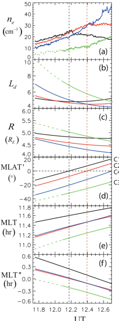
hrFig. 8.Quantities for each of the four CLUSTER spacecraft (black, red, green, and blue for C1, C2, C3, and C4, respectively) plotted as a function of UT,(a)nevalues inferred from the upper hybrid noise band,(b)Ld calculated using the dipole field model (Eq. 9) with the modified magnetic latitude MLAT′(Eq. 11),(c)the geocentric radiusR,(d)MLAT′,(e)magnetic local time MLT, and(f)the co-rotation local time MLT′′(Eq. 18).
UT
e
n
(
3)
cm−
(a) Fit 1, Power Law
(b) Fit 2, Quadratic in L and z
(c) Fit 5, like 2, but linear in UT’
C1
C2
C3 C4
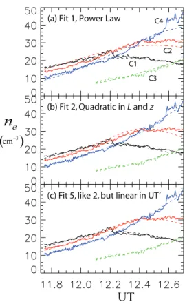
Fig. 9. Observed values ofne (solid curves) and model values (dashed curves) versus UT for all four CLUSTER spacecraft (black, red, green, and blue color for C1, C2, C3, and C4, respectively) for
(a)fit 1,(b)fit 2, and(c)fit 5 in Table 1.
1
2 4 5, 6
MLAT '
e,
n
Fig. 10. Parallel dependence ofne,ne,k, versus the magnetic lat-itude MLAT′for fits withne,ksymmetric with respect to MLAT′
(black curves): fit 1 (solid black curve), fit 2 (dotted black curve), and fit 5 (dashed black curve); and for asymmetric (with respect to MLAT′) dependencies (red curves): fit 4 (solid red curve), and fit 6 (dashed red curve).
In Fig. 9c, we compare the observed and model densities for fit 5. The agreement is good in most regions; there is still some disagreement for C2 (red curves) at the largest values of UT. This remaining disagreement is either because we have not used general enough model functions, or the assumption of separability in Eq. (6) is not exactly valid. Nevertheless,
L
1 2, 3, 5
e,
e,
(
5)
L L L
n
n
=Fig. 11. TheLddependence ofne,ne,Ld, normalized to its value atLd=5 is shown for fit 1 (solid black curve), fit 2 (blue dashed curve), fit 3 (red dashed curve), and fit 5 (green dashed curve).
we regard the fit shown in Fig. 9c to be very good. TheLd dependence for fit 5 is the dashed green curve in Fig. 11, and it’s clearly very close to the curves for fits 2 and 3 (blue and red dashed curves, respectively). The parallel dependence for fit 5 is the black dashed curve in Fig. 10. There is still a local peak inne at MLAT′=0, but the peak has slightly less amplitude (6% drop inne from the value at MLAT′=0 to the minimum value versus a 9% drop for fit 2). Fit 6 is the same as fit 5 (with terms for MLT′ and UT′) but with
asymmetric terms inz′allowed like for fit 4. That is, terms
forz′,z′2,z′3, andz′4were all included. Theχ and exp(χ )
values, 0.0430 and 1.044, respectively, were almost identical to those for fit 5 (0.0431 and 1.044, respectively), as shown in Table 1. The coefficients of the odd terms inz′(z′andz′3
) were very small compared to those of the even terms, so that the field line dependence was almost the same, as can be seen by comparing the red dashed curve (fit 6) to the black dashed curve (fit 5) in Fig. 10.
Fig. 12.Sounder data measured by the WHISPER instrument on the C1 spacecraft showing the labelled resonances.
odd terms inz′are included (fit 6), the resulting fit is nearly
identical to that of fit 5.
Now we return to Fig. 7, where we make use of the par-allel distribution ofne from fit 5. In Fig. 7a and b, the red curve is the product of theLd dependence of fit 5 evaluated atLd=4.8 (the L value of C1 at the time the Alfv´en fre-quencies were observed) and the parallel dependence of fit 5, n5,k. In Fig. 7c and d, the same values are plotted but
multiplied by 2.5 (to aid comparison to the curves forρ). Fit 5 forne has a local peak inne at the magnetic equator, likeρ, but the amplitude of the peak inneis smaller, a 6% drop inne from MLAT′=0 to the minimum value versus a 23% drop inρ for the solution based on the peak frequen-cies (thick solid black curve in Fig. 7a). Using this last curve forρ with the red curve forne, we can derive the average ion massM≡ρ/ne within the region of overlap in MLAT′;
Mis plotted in Fig. 7e and f. The value ofM is largest at MLAT′=0.
Some earlier work has indicated that the He+ density, which is usually small, is not nearly as sensitive to geomag-netic activity as is that of O+ (Craven et al., 1997; Krall et al., 2007). This suggests that ifM is significantly greater than unity,nO+/neis as a first approximation equal to(M−1)/15. Combining this relation with quasineutrality for an H+/O+ plasma (1=nH+/ne+nO+/ne), we can use the field line
dis-tribution ofMto derive the field line distribution of H+ and O+ and these curves are plotted in Fig. 7g and h. The field line distribution of H+ is less peaked than that ofne(3% peak for H+ versus a 6% peak forne), while the field line distribu-tion of O+ is more peaked than that ofρ (34% peak for O+ versus a 23% peak forρ).
6 Comparison to other density measurements
The purpose of this section is to check for consistency of the measured density values, and then to compare the two events. For consistency, the average ion massM≡ρ/ne should be greater or equal to 1 amu (corresponding to pure H+ plasma), and the directly measured heavy ions should be less than that needed to account for the mass density inferred from the Alfv´en wave frequencies.
6.1 Other measurements for 28 October 2002
1000 10000
O
+ (eV)
1000 10000
0.1 1.0
O
+ n (cm -3 )
1-40 (keV)
0100 0200 0300 0400
hhmm
8.7 12.8 73.8 5.5
8.6 5.7 65.3
4.9
8.8 4.8 63.0
4.7
9.2 8.7 70.1
5.1 MLT
L ILAT DIST
1 1000
1/cm
2 -s-sr-(eV/e)
CIS Instrument, CLUSTER SC1, 2002 Oct 28
Fig. 13.(Top) Spectrogram of the flux of O+ions with energy from 1-40 keV, and (bottom) density of O+ integrated over the same energy range for the 28 October 2002 event.
smoothed spectrum. The smoothing uses a common ad hoc filter function, providing in all regions a first approximation of the plasma frequency Fp. It is based on the fact that all res-onance peaks (Fce, Fqs, Fp, Fuh) appear in a frequency range more or less centered near Fp. A value of Fp between 23 and 27.2 kHz leads to an electron densityneof about 8 cm−3.
Oxygen ions (O+) can be detected using the Cluster Ion Spectrometry (CIS) instrument (R`eme et al., 2001). A spec-trogram of the flux of O+ions with energy from 1–40 keV is shown in the top panel of Fig. 13, and the density of O+ integrated over the same energy range is shown in the bottom panel. Below 1 keV, the signal to noise ratio was too low to get a reasonable estimate. At about 02:30 UT, the measured O+density is about 0.5 cm−3.
Table 4 summarizes our information about the 28 October 2002 event. The negativeDst value =−49 nT is indicative of a significant ring current population. The instantaneous
KpandhKpi3(average of previousKpvalues weighted with exp(−(t−tKp)/(3 days))) values (4.6 and 4.1, respectively) indicate a moderately high level of geomagnetic fluctuations. The C1 spacecraft was close to the magnetic equator (MLAT =−5.4◦), and the inferredρ at the spacecraft location was 37.6 amu/cm3 (Fig. 17c and Eq. 22). The shape of the field line distribution was flat in the middle region (around MLAT=0) and very steep at large|MLAT|(close to the iono-sphere), as shown in Fig. 16. Usingρ=37.6 amu/cm3 and
ne=8 cm−3, the average ion massM≡ρ/ne=4.7 amu. In a plasma composed of H+, He+ and O+, the average ion mass will be
M=1+3 n
He+ ne
+15
n
O+ ne
. (25)
To have a value ofM=4.7 would requirenO+/ne=0.25 in an H+/O+ plasma, or nO+=2 cm−3. If nHe+/ne=0.20 (a typical upper limit), nO+/ne=0.21 is needed, correspond-ing to nO+=1.7 cm−3. We observed nO+=0.5 cm−3 with
energy>1 keV, and the plot of the flux of O+ (bottom panel of Fig. 13) indicates that there is more O+ at lower energies. Thus we observed a substantial fraction of the needed O+, enough to raiseMto the valueMO+,obs=1.9 in Table 4, but
not enough to raise it toM=4.7.
6.2 Other density measurements for 10 September 2002
At the time of this event,ne=22 cm−3at the position of C1. From the solution based on the peak frequencies (thick solid curve) plotted in Fig. 7,ρ=63.0 amu/cm3there, leading to M=2.8. In this case, we were able to measure O+ down to 40 eV (Fig. 14), and find an integrated oxygen density
nO+=0.6 cm−3. The measured O+ is by itself enough to
raiseMto a value of 1.4. These values are listed in Table 4. As in the previous case, there is a significant amount of flux at the lower range of energy, so it is likely that there was more oxygen present. From Eq. (25), a value ofM=2.8 would re-quirenO+/ne=0.12 in an H+/O+ plasma, ornO+=2.7 cm−3
(as compared to 1.7–2 for the 28 October 2002 event). With
nHe+/ne=0.2 (a typical upper limit), there would need to be
nO+/ne=0.08, ornO+=1.8 cm−3(as compared to 1.7–2 for
the 28 October 2002 event). Based on these numbers, the to-tal amount of O+ could be similar for the two events. As can be seen in Fig. 14, there are two populations of O+, one with energy lower than 1 keV, and another with higher energy. About 0.5 cm−3of the total O+ (0.6 cm−3) is in the higher
Event UT MLT Dst Kp hKpi3 ρ Shape ne M nO+ MO+,obs
(Hours) amu
cm3
(cm−3) (cm−3)
28 Oct 2002 0233 8.7 −49 4.6 4.1 37.6 flat/steep 8 4.7 0.5 (>1 keV) 1.9
10 Sep 2002 1207 11.6 −61 3.6 2.7 62.6 slightly peaked (23%) 22 2.8 0.6 (>40 eV) 1.4
100 1000 10000
O
+ (eV)
100 1000 10000
1 1000
1/cm
2-s-sr-(eV/e)
0.10 1.00
O
+ n (cm -3)
40-40000 (eV)
1100 1130 1200 1230 1300 1330
11.2 7.8 69.0
5.4
11.4 5.8 65.4 5.1
11.5 4.9 63.2
4.9
11.7 5.0 63.4
4.8
11.9 6.2 66.3
4.8
12.0 9.6 71.2
4.9 hhmm
MLT L ILAT DIST
CIS Instrument, CLUSTER SC1, 2002, Sept 10
Fig. 14. (Top) Spectrogram of the flux of O+ ions with energy from 40 eV to 40 keV, and (bottom) density of O+ integrated over the same energy range for the 10 September 2002 event.
6.3 Comparison of the two events
The density of ring current (>1 keV) O+ is about the same for both cases and the total amount of O+ could be similar, but the electron density is larger for the 10 September 2002 event (22 cm−3as compared to 8 cm−3for 28 October 2002), leading to a smaller value ofMfor the 10 September 2002 event (2.8 as compared to 4.7 for the 28 October 2002 event). TheDst values for the two events are similar (Table 4), con-sistent with similar values for the O+ density with energy
>1 keV. The Kp value for the 10 September 2002 event is somewhat lower (3.6 as compared to 4.6 for the 28 October 2002 event). There is a greater difference inhKpi3(average
ofKp weighted with 3 day exponential decay as described in Sect. 3.3). The indicesDstandKpare plotted for the two events versus time in Fig. 15, showing thatKp was consis-tently higher during the two days leading up to the 28 Oc-tober 2002 event. This probably correlates with greater con-vection leading to lowerne even though for both events, the CLUSTER spacecraft are in the plasmatrough (based on IM-AGE EUV images not shown). In summary, the ring current
populations of the two events are similar (at least for O+), but the cold electron density is larger for the 10 September 2002 event, leading to a lower average ion massM.
7 Discussion
7.1 The difference in the two events
Before discussing the results for the field line distribution of density, we discuss the results presented in Sect. 6. Ideally, we would like to show that the value of mass densityρ in-ferred from Alfv´en wave frequencies is equal to the sum of measured ion densities. Unfortunately, we cannot show that because the ion composition instrument on CLUSTER does not measure the cold (∼eV energy) heavy ions (ions heavier than H+). (Given the heavy ion densities, we can infer the proton density from the electron densityne.) We have shown that the measured O+ densitynO+,obsleads to an average ion
28 Oct 2002 10 Sep 2002
Dst
Kp
Day of Month
Fig. 15.Dst (top) andKp(bottom) versus time for the 28 October 2002 (left) and 10 September 2002 (right) events, with the event time at the right side of each panel.
andρare at least possibly correct. In the two events consid-ered (Table 4), both of which were in the plasmatrough, the
Dstvalues and density of O+ with energy>1 keV were sim-ilar (see discussion in Sect. 6.2), and the total amount of O+ may also possibly be similar. The main difference between the two events seems to be that the total density was greater for 10 September 2002 than for 28 October 2002 (Table 4). Although the field line distribution is slightly peaked for 10 September 2002, both field line distributions are relatively flat compared to field line distributions studied by Denton et al. (2006) (23% peak for 10 September 2002 versus about a factor of 2 forL=6–8 in Fig. 8 of Denton et al.). Denton et al. found that the field line distribution of mass density was typically flat forL=4–5, but slightly peaked forL=5–6; the value ofLin this study, 4.8, is close to the boundary between these two ranges.
7.2 Variation in solutions for the mass density for 28 Oc-tober 2002
Here we consider how the solution for the field line depen-dence varies if we use different assumptions for the field line dependence or if we use a smaller number of harmonics. In Fig. 16, we show the solutions forρ using different num-bers of polynomial terms Npoly in Eq. (1). Solutions with
Npoly<7 are shifted down by factors of 10 so that the solu-tions do not overlap, as indicated in the caption. The three solid curves represent solutions using all the observed fre-quenciesNfreq=8, but the dotted curves are solutions using Nfreq=Npoly. (The vertical lines are there to help the viewer
more accurately compare the different curves.) There are no solid curves for Fig. 16 withNpoly≤4 because when using
8 input frequencies (Nfreq=8) our code only converged on
valid solutions when Npoly was at least 5. This is
proba-bly because the field line distribution of ρ is very flat for |MLAT|.20◦ but very steeply increasing with respect to
MLAT
(°)
3
amu
cm
7
6
5
4
3
2
1 Npoly=
Fig. 16. Solutions for mass density based on the peak frequencies fn−inputfrom Table 2. The numerical labels indicate the number of
polynomialsNpolyused in Eq. (1). The values ofρforNpoly<7 are
divided by 107−Npolyso that they do not overlap. The solid (dotted) curves show the solutions usingNfreq=8 (Nfreq=Npoly)
frequen-cies. The dashed curve is a second solution forNfreq=Npoly=6 as
described in the text.
|MLAT| for |MLAT|&40◦, and this distribution cannot be fit with a small number of polynomials. The solid curves forNpoly=5 and 6 are nearly identical. The solid curve for
Npoly=7 is very similar but increases less at the largest values of|MLAT|. Despite this, the solution forNpoly=7 still lies within the range of solutions for the Monte Carlo simulation withNpoly=5, as can be seen from Fig. 6b.
While there are no solutions forNpoly≤4 using all eight
input frequencies (Fig. 16), we can find solutions if we re-duceNfreq. The dotted curves in Fig. 16 show the solutions
using Nfreq=Npoly input frequencies. It is clear that using
are unique. In fact, forNfreq=Npoly=6, we found two
solu-tions. The second solution is the large dashed curve in Fig. 16 (that goes to the same values ofρas the otherNpoly=6 curves
at MLAT=0◦). However, the chances of finding solutions that differ are greatly reduced ifNfreq>Npoly because the extra
information constrains the values of the polynomial coeffi-cients. For that reason, theNpoly=5 or 6 solutions (which
are nearly identical) may actually be more accurate than the
Npoly=7 solution. (Though as we noted before, theNpoly=7 solution does lie within the range of the values from the Monte Carlo simulation usingNpoly=5.)
For the 28 October 2002 event, we have eight frequen-cies, but most often when mass density is inferred from Alfv´en frequencies, there is far less information available. To show how less information could influence the results, we show several different solutions forρ in Fig. 17. The bold solid curve is our solution withNpoly=5 (τ expansion)
with Nfreq=8. The thin solid curve is our solution using Npoly=3 with Nfreq=3. The dashed curves are found
us-ing only the fundamental frequency (Nfreq=1), and
assum-ing the power law form (Eq. 3) withα=1 (dotted), 2 (small dashes), 4 (medium dashes), and 6 (large dashes), as labelled in Fig. 17b. UsingNfreq=3, the three term polynomial solu-tion does a fairly good job of modelling the field line distri-bution up to|MLAT|=35◦, but does not model the steep in-crease at large|MLAT|(at ionospheric altitudes) represented in the 5 polynomial solution. Clearly the power law form does not well describe the variation ofρover the entire range of MLAT either. The field line distribution ofρis very flat within|MLAT|=20◦(thick solid curve), and the best power
law fit for this region is withα=1 (dotted curve). The value
α=6 (large dashes) yields best agreement at large|MLAT| (close to the ionosphere). If three frequencies are used to determine the best power law fit, the inferred power law co-efficient isα=2.25 and the resulting solution (not shown) is very close to the α=2 curve in Fig. 17 (found using only the fundamental frequency). As stated previously, our code does not converge on a valid solution usingNfreq=8 with the uncertainties in Table 2. However, if we increase the uncer-tainties by a factor of 10, we can find the best fitting power law solution, which hasα=4.05; the resulting solution (not shown) is very close to theα=4 solution in Fig. 17. Denton et al. (2006), using CRRES data, suggested thatα=2 was the best choice forL=4–5 if the power law form is used. These results also show thatα=2 would work fairly well for the 28 October 2002 event up to about|MLAT|=35◦. The use of a
power law solution withα=4 better represents the values of
ρat larger|MLAT|, but as can be seen from Fig. 17, this so-lution leads to equatorial and topside ionosphere values ofρ
that are too low, and mid-range values that are too high (com-paring theα=4 medium dashed curve with the thick solid curve).
(c) (d)
MLAT (˚) R R( E)
3 amu cm ⎛ ⎞ ⎜ ⎟ ⎝ ⎠
1 2 4
Fig. 17. The bold solid curve is our solution forρ versus MLAT (left) and geocentric radiusR(right) using 5 polynomial terms to fit the 8 peak frequencies in Table 2. The thin solid curve is the solu-tion using 3 polynomial terms to fit 3 frequencies. The four dashed curves are the solutions using only one frequency (the fundamen-tal) assuming the power law form (Eq. 3) forα=1 (dotted), 2 (small dashes), 4 (medium dashes), and 6 (large dashes), as labelled in(b). The bottom panels are the same as the top panels, except that the range ofρvalues plotted is smaller.
7.3 Discussion of the mass density field line distribution for 28 October 2002
For the 28 October 2002 event, we were able to determine a large number of harmonic frequencies with unprecedented precision. The resulting solution for mass density was also very precise because of the large number of harmonics mea-sured and the smaller relative uncertainties in the harmonic frequencies (Fig. 6). The net result is that the error in the inferred mass density is probably dominated by factors other than the uncertainty in frequency (e.g., magnetic field model and theoretical wave equation). As shown in Fig. 6, our solution for the field line distribution on 28 October 2002 (at L=4.8) is very flat for |MLAT|.20◦ but very steeply increasing with respect to |MLAT| for |MLAT|&40◦. Be-cause of the improved precision of the observed frequen-cies, we are able to see a steep increase inρ as MLAT ap-proaches ionospheric values (Fig. 5a and b). And because of this increase, the Alfv´en speed VA≡B/√4πρ (in CGS units) does not keep increasing as |MLAT| increases; the increase in ρ at large |MLAT| causes a decrease in VA at the largest values of|MLAT| as shown in the middle pan-els of Fig. 5. (Thus we observe the ionospheric Alfv´en res-onator (Polyakov, 1976; Lysak, 1993), a dip in the value of
(km)
h
(a) South
(b) North
3 amu cm
⎛ ⎞ ⎜ ⎟ ⎝ ⎠
IRI
ρ
+
IRI-O ρ
Fig. 18. The solid curves are the same solutions forρ that were plotted in Fig. 5a and b, but shown with respect to heighthfrom the Earths surface within the southern(a)and northern(b)ionospheres. The large dashed curve is the mass density from the International Reference Ionosphere (IRI) model (Bilitza, 2001). The dotted curve is the mass density from the IRI due to O+.
affects the solutions for the frequency of the Alfv´en wave harmonics. This can be seen from the values of τ (the Alfv´en crossing time coordinate defined in Eq. 2) shown in Fig. 5e and f. In the WKB approximation, the Alfv´en fre-quency∼1/(RSNds/VA)=τN−τS, where the integral is eval-uated from the southern ionosphere (S) to the northern iono-sphere (N). The contribution to τN−τS in each differential change in latitude dMLAT goes like the slope ofτ in Fig. 5e, and the slope ofτ versus MLAT is non-negligible at every value of MLAT, showing that all regions of MLAT contribute to the Alfv´en frequencies. This is the second reason for the improved precision at large values of|MLAT|; the values ofρ at large |MLAT|are having a significant effect on the frequencies. (In our previous solutions (e.g., Denton et al., 2004),ρdid not increase nearly so much at large|MLAT|so thatVAbecame very large at large|MLAT|(due to the large value ofBat low altitude) and the differential contribution to
τ,dτ=ds/VA, became small.)
Considering the tremendous imprecision of our previous solutions at large values of |MLAT| (Denton et al., 2001, 2004, 2006; Takahashi et al., 2004; Takahashi and Denton, 2007), one might well question whether our technique can actually determine a variation inρ of more than four orders of magnitude. While we cannot prove that this field line dis-tribution ofρ is accurate, several pieces of evidence argue that the values ofρmay actually increase steeply as we have found. First of all, we do not find valid solutions for the field line distribution of log10ρ using less than five
polyno-mial terms. (We also do not find a solution using the power law description withρ∼R−α.) Secondly, polynomial fits to
ρ(rather than log10ρ) did not yield valid solutions, indicat-ing that we need a functional form that can represent a very steep increase inρat large values of|MLAT|. Third, the dis-tribution seems to have converged with respect toNpoly for Npoly=5. Fourth, the values ofρ that we find at the largest
values of|MLAT|compare reasonably well with ionospheric mass densities. This is shown in Fig. 18 for the southern (a) and northern (b) ionospheres. Note that our values ofρ
are intermediate between the IRI values at heighth.600 km and those ath&1400 km. Therefore, our estimate of mass density based on Alfv´en frequencies may be probing into the ionosphere while not resolving its detailed structure.
Further work should be done to verify whether the four or-der of magnitude variation inρwith respect to MLAT is justi-fied based on our method, but it is encouraging that the iono-spheric values ofρ are consistent with values from the IRI model. Such a dependence with increasing steepness away from the magnetic equator is also consistent with the field line dependence ofneinferred from active radio sounding by IMAGE RPI (Reinisch et al., 2004; Denton et al., 2006, and references therein). An important effect of the steep increase inρat large|MLAT|is that the large|MLAT|(low altitude) portion of the field line contributes to the global frequency of oscillation, even for the fundamental mode (Fig. 5e). 7.4 Discussion of the field line distribution of mass
den-sity for 10 September 2002
For the second event, 10 September 2002, we measured only three harmonic frequencies and the solution was not as ac-curate (partly because of the small number of Alfv´en wave harmonics observed). In this case, we found a small local peak in mass density near the magnetic equator. This peak is similar to those we have found in earlier studies, but smaller in amplitude, 23% (as compared to a factor of 2 in the after-noon local time sector at largeL&6 (Takahashi and Denton, 2007)). Because this peak is small, and because the range of solutions from the Monte Carlo simulation does not exclude a flat distribution (Fig. 7), we would be reluctant to confi-dently state that this peak is real based on this data alone. However, our analysis of the field line distribution of elec-tron density for this event also indicates that the density is peaked at the magnetic equator.
7.5 Discussion of the electron density distribution for 10 September 2002