Structure of Interest Rates
Luiz Paulo Fichtner
Nova School of Business and Economics
Universidade Nova de Lisboa
A thesis submitted for the degree of
Doctor of Philosophy
List of Figures iii
List of Tables v
1 Out-of-Sample Predictability of Bond Returns 1
1.1 Introduction . . . 1
1.2 Forecasting Returns with Predictive Regressions . . . 4
1.2.1 Notation . . . 4
1.2.2 Yield Forecasting Approach . . . 5
1.2.3 Forecasting Performance . . . 7
1.3 Empirical Analysis . . . 7
1.3.1 Data and Predictors . . . 7
1.3.2 Results . . . 9
1.3.3 Robustness Check . . . 11
1.4 Conclusion . . . 13
1.5 Tables and Figures . . . 14
2 How You Estimate the Yield Curve Matters! 23 2.1 Introduction . . . 23
2.2 Methodology . . . 26
2.2.1 A two-factor CIR model for the Euribor . . . 26
2.2.2 Interest rate forecasts . . . 28
2.2.3 Interest rate caps . . . 28
2.2.4 Econometric method . . . 30
2.3 Empirical Analysis . . . 33
2.3.1 Data . . . 33
2.3.2 Results . . . 33
2.4 Conclusion . . . 37
2.5 Tables and Figures . . . 38
3 Bias and the Estimation of the CIR Term Structure Model 47 3.1 Introduction . . . 47
3.2 Methodology . . . 51
3.3 Results . . . 55
3.4 Conclusion . . . 59
3.5 Tables and Figures . . . 61
Bibliography 75
1.1 FB and Random Walk bond excess return forecasts . . . 21
1.2 CP and DNS bond excess return forecasts . . . 22
2.1 CIR cap prices with Alpha = 0.1 . . . 42
2.2 CIR cap prices with Alpha = 0.3 . . . 43
2.3 CIR cap prices with Alpha = 0.5 . . . 44
2.4 CIR cap prices with Alpha = 0.7 . . . 45
2.5 CIR cap prices with Alpha = 0.9 . . . 46
3.1 Relationship between k and option and bond prices . . . 73
3.2 Relationship between k and log-likelihood values . . . 74
1.1 Yield Curve Summary Statistics . . . 14
1.2 Fama and Bliss Excess Return Regressions . . . 15
1.3 Ilmanen Excess Return Regressions . . . 16
1.4 Cochrane and Piazzesi Excess Return Regressions . . . 17
1.5 Greenwood and Vayanos Excess Return Regressions . . . 18
1.6 Yield Forecasting Excess Return Predictions . . . 19
1.7 Fama and Bliss versus Dynamic Nelson Siegel Excess Return Predictions . 20 2.1 Euribor Zero Curve Summary Statistics . . . 38
2.2 Estimation of two-factor CIR model . . . 39
2.3 Pricing and Forecasting Errors . . . 40
2.4 Cap Volatilities . . . 41
3.1 Estimation of one-factor CIR model, √V = 0 b.p. . . 61
3.2 Estimation of one-factor CIR model, √V = 5 b.p. . . 62
3.3 Estimation of one-factor CIR model, √V = 10 b.p. . . 63
3.4 One-factor CIR model Pricing Errors . . . 64
3.5 Partial derivatives of the one-factor CIR model . . . 65
3.6 Estimation of two-factor CIR model, √V = 0 b.p. . . 66
3.7 Estimation of two-factor CIR model, √V = 5 b.p. . . 68
3.8 Estimation of two-factor CIR model, √V = 10 b.p. . . 70
3.9 Two-factor CIR model Pricing Errors . . . 71
3.10 Partial derivatives of the two-factor CIR model . . . 72
Out-of-Sample Predictability of
Bond Returns
1.1
Introduction
Significant predictability of bond returns is a much established fact in the literature. Cochrane and Piazzesi (2005) find that a single tent-shaped linear combination of for-ward rates predicts excess returns on one- to five-year maturity bonds with R-square up to 44%. They strengthen the results by Fama and Bliss (1987) and Campbell and Shiller (1991) against the Expectation Hypothesis of the Term Structure (EH). Based on a modified version of the EH, in which expected bond excess returns are unforecastable, Fama and Bliss test whether forward rates have information about expected returns on bonds with different maturities. They find that the spread between the n-year forward rate and the one-year yield predicts the one-year excess return of then-year bond, with R-squares up to 18%. Using a comparable approach, Campbell and Shiller (1991) find similar results forecasting yield changes with yield spreads. Following the bond return predictability literature, Ilmanen (1995) forecasts out-of-sample bond excess returns for different countries using the term spread, real yields, the inverse relative wealth, and bond return betas. He finds that these variables predict monthly bond excess returns with out-of-sample R-squares up to 12%.1 Greenwood and Vayanos (2008) find that, consistent with a preferred habitat model of the term structure, where clienteles with
1Ilmanen (1995) also uses international weighted averages versions of these variables. But due to data
availability for our samples, and because we found no impact of these variables for the data available, we chose to use only US variables.
strong preferences for specific maturities trade with arbitrageurs, the supply of long-relative to short-term bonds positively predicts long-term excess returns even after con-trolling for the term spread and Cochrane and Piazzesi’s single factor.
In this paper we assess the out-of-sample predictive power of the methods proposed by these authors for one-year holding period excess return regressions. We use Fama-Bliss monthly one- to five-year zero coupon bond prices (available from CRSP), from January 1965 to December 2010. On this dataset, we replicate the regressions of Fama and Bliss (1987), Ilmanen (1995), Cochrane and Piazzesi (2005), and Greenwood and Vayanos (2008), and forecast one-year holding period excess returns using only data available at the time of the forecast.1 This is the only approach that could have been implemented to time the market in real time. Judging by the R-square values, the models do well in explaining bond excess returns in sample. The Fama and Bliss regression produces squares of up to 15%, Ilmanen and Greenwood and Vayanos regressions produce R-squares of up to 31%, and Cochrane and Piazzesi’s regression reach R-R-squares of up to 33%.
However, hight in-sample R-squares do not imply good out-of-sample performance. Using the metric proposed by Goyal and Welch (2003), we find that all methods, except for Fama and Bliss, produce negative out-of-sample R-squares. Fama and Bliss’ method produces out-of-sample R-squares of up to 8.5%. Ilmanen’s regressions produce negative out-of-sample R-squares for the two- and five-year bond returns, while small, but positive out-of-sample R-squares for the three- and four-year bond returns. Cochrane and Pi-azzesi’s single factor regression produces out-of-sample R-squares of -8.5%. Greenwood and Vayanos’ regressions have the worst performance, with out-of-sample R-squares of -11%. Since the regressions try to minimize squared errors, they tend to overfit in sam-ple.2 Sampling noise in the data make regression coefficients not robust out of sample. Furthermore, the data is also prone to pure measurement error. In practice, discount bond prices at exactly the desired maturities are not observed. Instead, they must be
1Campbell and Shiller (1991) perform regressions based on yield spreads and these behave similarly
to Fama and Bliss’ regression. Thus, for simplicity, we only reproduce Fama and Bliss (1987).
2Ashley (2006) shows that the unbiased forecast is no longer squared-error optimal in this setting.
Instead, the minimum-MSE forecast is shown to be a shrinkage of the unbiased forecast toward zero. However, applying shrinkage to our regressions did not alter significantly the results. We therefore chose not to report shrinked out-of-sample R-squares.
estimated from observed bond prices. If excess return components are also used as right-hand-side variables, as in the case of Fama and Bliss’s forward spread and Cochrane and Piazzesi’s single factor, measurement error will induce spurious common movement in left- and right-hand-side variables. Although Cochrane and Piazzesi (2005) argue that the results of their single factor approach are not driven by measurement error, our out-of-sample results suggest that this and overfitting make their approach useless to forecast returns in practice.
In this paper we propose a different method for predicting bond excess returns. Instead of regressing returns on a set of explanatory variables, we forecast the relevant return components separately. By definition, the one-year holding period log excess return on a n-year bond at timet+ 1 is the difference betweenn times then-maturity bond yield at timet, and the sum ofn−1 times the (n−1)-maturity bond yield at time t+ 1 and the one-year bond yield at time t. It is straightforward to see that, at timet, the (n−1)-maturity bond yield at time t+ 1 is the only unknown. We forecast these bond yields to produce bond return forecasts. We use two yield forecasting approaches. First, simply we assume that yields follow a random walk. Substituting the random walk yield forecast in the excess return definition, the excess return forecast at time t+ 1 will be equal to the forward spread at timet. Although very simple, this approach produces out-of-sample R-squares of up to 15%. It also strengthens the idea that overfitting and measurement errors affects bond excess return forecasts based on predictive regressions. Fama and Bliss use the lagged forward spread in their excess return predictions, but assuming that yields follow a random walk is equivalent to taking the forward spread directly as the return forecast. Second, we forecast future yields using a dynamic Nelson Siegel model proposed by Diebold and Li (2006). This approach is highly tractable, and produces reasonable out-of-sample yield forecasts.1 Out-of-sample R-squares reach up to 24% with the dynamic Nelson Siegel approach using the Fama-Bliss dataset.
To verify the robustness of our findings, we test the out-of-sample predictive power of the Fama and Bliss (1987) and dynamic Nelson Siegel methods on a second dataset, namely Gurkaynak et al. (2006) monthly one- to twenty-year zero coupon bond prices (available from the Federal Reserve Board), from July 1982 to December 2010. This
1The out-of-sample R-square measure depends exclusively on the historical sample mean and the
forecasting errors. Since our approach is to forecast yields separately and plug them back into the excess return equation, the results are independent of the method used to forecast yields.
dataset enables us to evaluate the models using a more representative cross-section of the term structure of bonds, albeit for a shorter time series. When the Fama and Bliss model is estimated using this smaller sample, regression coefficients are no longer significant and out-of-sample R-squares are negative for all maturities. The three- and five-year bond excess return regressions that share a common sample between both datasets produce out-of-sample R-squares of -33% and -29%, respectively, in comparison to 7% and 8.5% in the Fama-Bliss dataset. On the other hand, the dynamic Nelson Siegel approach benefits from using a larger cross-section of bond yields in its estimation and produces out-of-sample R-squares of up to 30%.
The paper proceeds as follows. Section 3.2 discusses the notation, the methodology of the traditional predictive regressions and the performance measure. Section 1.3 describes the data, the main empirical results and the robustness check. Section 3.4 concludes.
1.2
Forecasting Returns with Predictive Regressions
The central goal of this paper is to assess the performance of existing Bond return predictability models, and compare them with our yield forecasting method. For this purpose, we need to evaluate models both by their in-sample and their out-of-sample performance. We begin this section by describing the notation and predictive regression methodology that we are using throughout the paper.
1.2.1 Notation
We use the same notation as CP and denote log bond prices as:
p(tn)= log price of n-year discount bond at time. (1.1)
Parenthesis are used to distinguish maturity from exponentiation in the superscript. The log yield is:
yt(n) ≡ −1 np
(n)
t , (1.2)
and the log forward rate at timetfor loans between time t+n−1 andt+nis:
ft(n)≡pt(n−1)−p(tn). (1.3)
The log holding period excess return from buying an n-year bond at time tand selling it as ann−1 year bond at time t+ 1 is:
rt(n+1) ≡pt(+1n−1)−p(tn)−y(1)t . (1.4) Bold letters denote vectors. When used as right-hand-side variables, these vectors include an intercept. The traditional predictive regression methodology regresses excess returns on lagged predictorsXt−1:
rt=β⊺Xt−1+εt.
We generate out-of-sample forecasts of the vector of log bond excess returns using a sequence of expanding windows, starting with an initial sample of five years. We use a subsample t= 1, ..., sof the entire sample of T observations and estimate the model. The forecast of the one-year excess log return at time s+ 1 is the estimated coefficient (denoted with hat) times the contemporaneous value of the predictor:
b
rs+1= βb⊺Xs.
1.2.2 Yield Forecasting Approach
We propose a new method for predicting log bond excess returns. We rewrite the one-year bond excess return definition in (1.4) in terms of yields:
rt(+1n) = (n−1)yt(+1n−1)−nyt(n)−yt(1). (1.5)
It is straightforward to see from the equation above that, at time t, yt(+1n−1) is the only unknown. Our approach is to forecastyt(+1n−1)and replace it in the excess return definition to produce our excess return forecast. We use two methods to forecast yields. First, we assume that yields follow a random walk. In this way, we do not need to estimate a yield forecast for every period in our out-of-sample procedure. Assuming a random walk for bond yields, we can write our excess return forecast as
b
rt(+1n) = (n−1)yt(n−1)−nyt(n)−yt(1).
Using the definitions in (1.2) and (1.3), we rewrite the equation above as:
b
rt(+1n) =ft(n)−yt(1). (1.6)
That is, the random walk excess return forecast equals the forward spread. In essence, we are using the same component as Fama and Bliss (1987), except that we do not run a regression, but instead use the forward spread directly as our return forecast. Second, we forecast yields using a dynamic Nelson Siegel model proposed by Diebold and Li (2006). Diebold and Li extend the the Siegel and Nelson (1988) model to an out-of-sample forecasting exercise. The Nelson-Siegel approach assumes that forward rates (and thus yields) can be characterised by a continuous function with only four parameters, as a polynomial times an exponential decay term.1 They fit the yield curve using the three factor model
y(tn)=Lt+St
1−e−λtn
λtn
+Ct
1−e−λtn
λtn −
e−λtn
. (1.7)
Where λt governs the exponential decay terms. To estimate their model, they fix the
parameter that governs the exponential decay rates at 0.0609. This value maximizes the loading on the curvature factor at 30 months. By fixing λt, they are able to estimate
the remaining parameters by ordinary least squares. Diebold and Li interpret the other three parameters Lt, St and Ct as latent dynamic factors, and show that they relate
to the level, slope and curvature of the yield curve, respectively.2 Repeating this for every period, they are left with a time series of estimated factors.3 Each factor is then modelled and forecasted separately as an univariate AR(1) process using a sequence of expanding windows, starting with an initial sample of five years. This method relates nicely to our return forecasting method, and has also a series of advantages, notably its tractability. The dynamic Nelson-Siegel one-year yield forecast is thus the summation of each latent factor forecast times its loading:
b
y(t+1n) =Lbt+1+Sbt+1
1−e−λn
λn
+Cbt+1
1−e−λn
λn −e
−λn. (1.8)
Using (1.5), it is possible to show that return forecast errors using both yield forecasting approache are simply yield forecast errors multiplied by the maturity:
rs+1−brs+1 = (n−1)
ys(n+1−1)−yb(sn+1−1). (1.9)
1Integrating these forward rates results in the corresponding zero-coupon yields.
2Diebold and Li (2006) define the level as the 10-year yield, the slope as the difference between
the 10-year and 3- month yields, and the curvature as the twice the 2-year yield minus the sum of the 3-month and 10-year yields.
3Using our data sample, we found the relation between the estimated factors and the level, slope
and curvature definition of Diebold and Li (2006) weak (considering that the dataset contains only one to five-year yields).
1.2.3 Forecasting Performance
We evaluate the performance of the forecasting exercise with an out-of sample R-square as in Goyal and Welch (2003) and Ferreira and Santa-Clara (2011).
R2 = 1− M SER M SEM
.
M SER is the mean squared error of the out-of-sample predictions from the model:
M SER=
1 T−s0
TX−1
s=s0
(rs+1−brs+1),
and M SEM is the mean squared error of the historical sample mean:
M SEM =
1 T−s0
TX−1
s=s0
(rs+1−rs),
where rs is the historical mean of excess log returns up to time s. Note that the
out-of-sample R-square will take negative values when the historical sample mean predicts returns better than the model.
1.3
Empirical Analysis
1.3.1 Data and Predictors
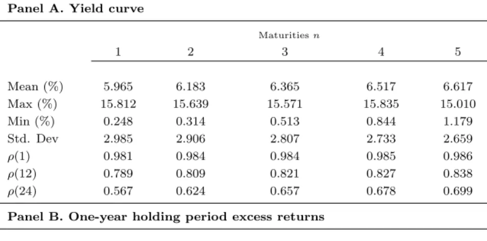
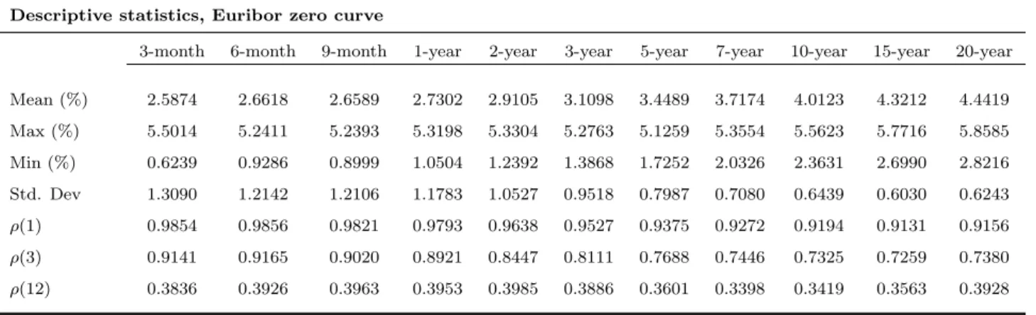
We use the Fama-Bliss dataset (available from CRSP) of monthly one- through five-year zero coupon bond prices, from January 1965 to December 2010. Monthly values are derived from end-of-month observations. From this dataset we compute one-year holding period returns. The one-year risk-free rate is assumed to be the one-year zero-coupon yield. Table 2.1 presents summary statistics for the yield curve and the one-year holding period returns. The descriptive statistics of yields in panel A present stylised facts known to the yield curve. The yield curve is on average upward sloping, long yields are less volatile than short yields, and yields of all maturities are very persistent (long yields are more persistent than short yields). The bottom three rows of the descriptive statistics show autocorrelations at displacements of 1, 12, and 24 months. For our one-year forecast horizon, autocorrelations are around 0.80 across maturities. The descriptive statistics of bon returns in Panel B shows that an investor who purchased 5-year bonds and sold them 12 months later earned on average 1.94% yearly in excess of the risk free
rate. The maximum holding period excess return was 16.89% for the 5-year bond in March 31, 1986. Holding period returns are more volatile than yields. The standard deviation of the 5-year bond yield is 2.66%, while the standard deviation of the one-year holding period return on a 5-year bond is 5.74%. This and the high persistence of yields is what makes our approach work well.
We also collect data on bond characteristics (issue date, coupon rate, maturity, calla-bility features) as well as monthly observations of face value outstanding from CRSP, from January 1965 to December 2010. For predictive variables that are not derived bond yields, we use the dataset updated maintained by Goyal and Welch (2003).1 From this
dataset we draw monthly observations of the market return (proxied by the S&P 500 continuously compounded returns, including dividends), and inflation.
The bond return predictors are:
Forward rate (f ): the log 1-year forward rate at time t for loans between time t+n−1 and t+n.
Forward spread (fs): The forward spread is defined as the difference between the forward rate and the one-year yield.
Term spread (ts): Then-year term spread is defined as the difference between the n-year bond yield and the one-year yield.
Real bond yield (ry): The real bond yield is defined as the difference between the current yield and annual year-on-year inflation:
Bond beta: The bond beta is the slope coefficient from a regression of excess bond returns on excess stock stock returns.
Inverse relative wealth (InvRelw): The inverse relative wealth is the ratio of past to current real wealth. Ilmanen (1995) motivates the use of this measure as a proxy for time-varying risk aversion. Asset risk premia should be positively related to aggregate relative risk aversion levels as suggested in Constantinides (1990), and Cochrane and Campbell (1999). We follow Ilmanen (1995) and use the real stock market index as a empirical proxy for aggregate wealth. The InvRelw is computed using an exponentially weighted average of past wealth levels, with a smoothing coefficient value of 0.90.2
1This data is maintained and updated by Amit Goyal at http://www.hec.unil.ch/agoyal/ 2I nvRelw
t≡
Pt−1 i=10.9
i−1W t−i
Wt .
Cochrane and Piazzesi factor (γ⊺f
t): The Cochrane and Piazzesi factor is
esti-mated by running a regression of the average (across maturities) excess return rt+1
on all forward rates:
rt+1 =γ⊺ft+ǫt+1. (1.10)
The Cochrane and Piazzesi factor is defined asbγ⊺f t.
Relative supply of long-term bonds (D10t +/Dt): Greenwood and Vayanos (2008)
define the relative supply of long- to short-term bonds as the ratio between total outstanding payments in ten years or longer and total outstanding payments.1 For this purpose, we replicate their indicator by collecting data on every U.S. government bond that was issued from 1965 from the CRSP historical bond database.
1.3.2 Results
We first reproduce the models of the existing literature.2 Table 1.2 presents the estimated coefficients from the Fama and Bliss (1987) regressions of bond excess returns on the forward spread, test statistics and out-of-sample R-squares. We follow Cochrane and Piazzesi (2005) and compute standard errors following Newey-West (1987), allowing for 18 months of lags. This covariance matrix is positive definite in any sample, giving more weight to more recent lags.3 We find results very similar to those of Fama and Bliss (1987). The forward spread coefficients are close to one, and the level coefficients are close to zero. Cochrane (2005) shows that a one-for-one variation of the expected excess return on an-maturity bond and the forward spread on the same-maturity bond is equivalent to the n-year yield following a random walk.4 The χ2 statistics for joint parameter significance are above the 1-percent critical value of 6.64, with the exception of the coefficient for the 5-year return, which is only significant at the 5-percent level. The in-sample R-squares are 11.6%, 13.2%, 14.9% and 7.3% for the 2, 3, 4 and 5-year bond excess returns, respectively. These results are also similar to the regressions in
1Outstanding payments at time tare the sum of principal and coupon payments from all bonds,
bills, and notes that were issued at timetor before and have not yet retired, scaled by their face value outstanding.
2We use the Matlab code from Cochrane and Piazzesi (2005), available at John Cochrane’s website:
http://faculty.chicagobooth.edu/john.cochrane/research/.
3We also compute Hansen-Hodrick (1980) standard errors that explicitly control for overlapping
observations, imposing equal weights on the first 12 lags. However, because both measures were very similar, we use only the first. We use the Newey-West 18 lag standard errors for joint test statistics.
4Replace the bond excess return definition in (1.6).
Cochrane and Piazzesi (2005) who replicate the Fama-Bliss regression to compare it to their single-factor model. Both studies argue that positive slope coefficients and high R-squares prove that returns are predictable and thus violate the Expectations Hypothesis. Figure 1.1 plots the 5-year bond excess return forecasts of the Fama and Bliss and random walk approaches against actual excess returns. It is clear from this figure that the Fama and Bliss excess return forecast converges to the random walk excess return forecast over the sample period and that the random walk approach performs much better at the beginning of the sample. Out-of-sample R-squares for the Fama and Bliss approach are 2.4%, 7.0%, 8.5% and 4.0% for the 2, 3, 4 and 5 years, respectively.
Second, we analyse the regressions with the predictive variables of Ilmanen (1995). Ilmanen proposed using variables linked to yields, such as the yield spread and real yields, but also variable linked to risk and risk aversion, such as the bond beta and the inverse relative wealth. Like our study, Ilmanen assesses the out-of-sample power of his regression. Using one-month holding period returns, he finds out-of-sample R-squares up to 12%.1 Table 1.3 presents the results for the one-year holding period return regressions.
Regression coefficients are jointly significant at the 1-percent level. Compared to Fama and Bliss, in-sample R-squares are much higher, around 30%. On the other hand, the out-of-sample R-squares produced using Ilmanen’s regressions are much lower, at -5.6%, 1.3%, 2.4% -2.5% for the 2, 3, 4 and 5 years, respectively.
Table 1.4 presents results for the Cochrane and Piazzesi (2005) regressions. They use a two-step procedure in their regressions in order to capture the single-factor structure for return forecasts. They find that the this two-step procedure has little effect on the excess return regression estimated coefficients, but adds economic meaning. Their return-forecasting single tent-shaped factor is unrelated to the usual term structure factors of level, slope and curvature. The table shows the regression coefficients and test statistics for the holding period excess return regressions on the single-factor. Coefficients are jointly significant and in-sample R-squares are as high as 32.6%. The out-of-sample R-squares on the other hand are negative for all maturities. Out-of-sample R-squares are as low as -8.5%, underperforming the historical average return.
1The yield forecasting approach based on yields following a random walk produces out-of-samples
R-squares as high as 92%, using monthly bond returns. This is because yield forecasting errors decrease with the forecasting horizon, making return forecasts more accurate.
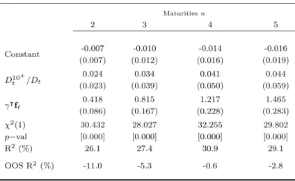
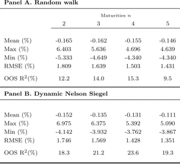
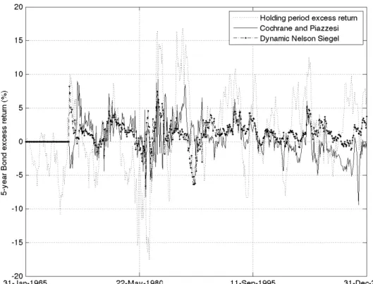
Greenwood and Vayanos (2008) find that, in accordance to a preferred habitat theory of the term structure, the supply of long- relative to short-term bonds helps to explain future bond excess returns. In addition to this variable, they also include the Cochrane and Piazzesi (2005) single-factor and the term spread. Table 1.5 presents the results of the Greenwood and Vayanos regression.1 All regression coefficients are jointly significant at the 1-percent level. Like the previous regression, in-sample R-squares are high, up to 30.9% for the 4-year return, but out-of-sample R-squares are negative for all maturities. The models above do badly in predicting excess returns out of sample. With excep-tion of the Fama and Bliss method which converges to the random walk excess return forecast, the models fall short of a forecast based on the historical sample mean. Table 1.6 presents the results for the yield forecasting approach. Panels A and B present sum-mary statistics of yield forecasts and out-of-sample R-squares for the random walk and dynamic Nelson Siegel approaches, respectively. For both forecasting methods, mean residuals are negative. This reflects the fact that the average yield curve is upward slop-ing, and both methods have poor performance predicting negative slopes of the yield curve. The summary statistics results are reflected in the overall out-of-sample perfor-mance. The random walk predicts excess returns with R-squares of up to 15.3%, while the dynamic Nelson-Siegel predicts excess returns with R-squares of up to 23.6%. Figure 1.2 plots the 5-year bond excess return forecasts against the actual excess returns for the Cochrane and Piazzesi’s and dynamic Nelson-Siegel approaches. From figures 1.1 and 1.2 it is possible to see that the yield forecasting approach performs much better than the traditional predictive regression in forecasting bond excess returns.
1.3.3 Robustness Check
As a robustness check of our findings, we conduct the out-of-sample exercise for the Fama and Bliss (1987) and dynamic Nelson Siegel methods on the Gurkaynak, Sack, and Wright dataset of monthly one- to twenty-year zero coupon bond prices (available from the Federal Reserve Board), from July 1982 to December 2010.23 This dataset enables
1The regression using the term spread instead of the single-factor yielded similar results.
2Thirty-year zero-coupon bond yields are available only from November 1985. We incorporate the
twenty-one- through thirty-year yields in the dynamic Nelson-Siegel forecast, from January 1986 onwards.
3Note also that the the maturities we use are equally spaced, unlike Diebold and Li (2006) which
use a dataset containing maturities with lower frequencies at the short end of the yield curve. Implicitly, they are weighting the short end of the yield curve more when fitting their model. Although using
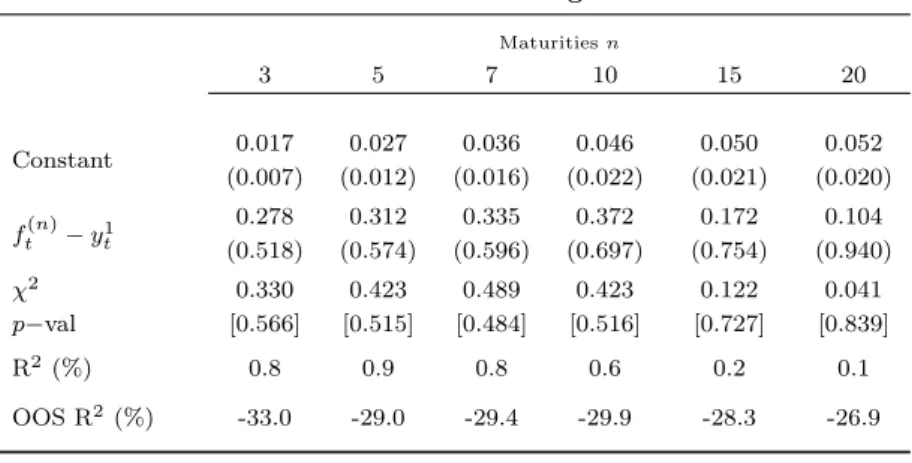
us to evaluate the models using a more representative cross-section of the term structure of bonds, albeit for a shorter time series. For simplification, we report only the 3, 5, 7, 10, 15 and 20-year returns. Despite being constructed using different bootstrapping and smoothing techniques than the Fama-Bliss dataset, one to five-year yields for the overlapping period are very close. This makes three and five-year return regressions comparable across datasets. Panel A in Table 1.7 presents the estimated coefficients from the Fama and Bliss regressions of bond excess returns on the forward spread, test statistics and out-of-sample R-squares. The Fama and Bliss model performs much worse in this second dataset. Forward spread coefficients are far from one even for the three and five-year bond excess return regression that share a common sample. Regression coefficients fail the joint significance test at any level, and in-sample R-squares are only marginally positive. The small sample bias is more acute in the second, smaller, sample. Negative out-of-sample R-squares (as low as -33%) is evidence that the models overfit in sample, and thus underperform out of sample.
Panel B presents summary statistics of yield forecasts and out-of-sample R-squares for the dynamic Nelson Siegel approach. Mean residuals are negative, reflecting the fact that the model is still deficient predicting negative slopes for the yield curve. Yield RMSE are much smaller than for the Fama-Bliss dataset. Clearly, the dynamic Nelson Siegel approach benefits from estimating Lt, St and Ct using a larger cross-section of
bond yields and thus produces better yield forecasts. The summary statistics results are reflected in the overall out-of-sample performance. Out-of-sample R-squares are positive for all maturities, reaching values of up to 29.8% for the seven-year bond return. Interestingly, in spite of having lower yield forecasting RMSE than for other maturities, the out-of-sample R-squares for the 15- and 20-year bond returns are only 15.3% and 8.7%, respectively. This is because the excess return forecasting error for then-maturity bond is (n−1) times the yield forecasting error, and MSE are penalised by (n−1)2.
Thus even though the yield forecasting improves with maturity, out-of-sample R-squares will be smaller.
equally spaced is not necessarily optimal (we underestimate the short end variation of the yield curve), our aim is just to produce better forecasts than the random walk approach, to show the power of the yield forecasting approach for bond returns.
1.4
Conclusion
Bond returns have long been thought to be predictable. Nevertheless, the existing liter-ature lacks out-of-sample evidence. Our paper closes this gap. We assess the predictive power for one-year holding period bond excess return regressions of Fama and Bliss (1987), Ilmanen (1995), Cochrane and Piazzesi (2005) and , Greenwood and Vayanos (2008). We find that high in-sample R-squares are a misleading indication of out-of-sample predictability. Problems arising from sampling errors in the data cause regres-sions to overfit in sample, and underperform out of sample.
We propose a new approach for predicting bond excess returns. Instead of forecasting returns directly, we forecast bond yields and replace them in the bond excess return definition. We use two bond yield forecasting methods: a random walk and a dynamic Nelson-Siegel approach proposed by Diebold and Li (2006). Both approaches outperform return forecasts based of the existing literature. An investor who used a simple random walk on yields would have predicted bond excess returns with R-squares of up to 15%, while a dynamic Nelson-Siegel approach would have produced R-squares up to 30%.
1.5
Tables and Figures
Table 1.1: Yield Curve Summary Statistics
This table reports summary statistics for yields and one-year holding period excess returns of Fama-Bliss yields from CRSP, from January 1965 to December 2010, with bond yields of maturities of 2 to 5 years. The last three rows of Panel A contain sample autocorrelations at displacements of 1, 12, and 24 months.
Panel A. Yield curve
Maturitiesn
1 2 3 4 5
Mean (%) 5.965 6.183 6.365 6.517 6.617
Max (%) 15.812 15.639 15.571 15.835 15.010
Min (%) 0.248 0.314 0.513 0.844 1.179
Std. Dev 2.985 2.906 2.807 2.733 2.659
ρ(1) 0.981 0.984 0.984 0.985 0.986
ρ(12) 0.789 0.809 0.821 0.827 0.838
ρ(24) 0.567 0.624 0.657 0.678 0.699
Panel B. One-year holding period excess returns
Mean (%) 0.500 0.880 1.151 1.209
Max (%) 5.968 10.261 14.381 16.889
Min (%) -5.595 -10.426 -13.545 -17.548
Std. Dev 1.837 3.368 4.674 5.737
Table 1.2: Fama and Bliss Excess Return Regressions
This table reports coefficient estimates and corresponding statistics for regressions of one-year holding period excess returns on constant maturity Treasury Bonds on the forward spread (ft(n)−y1
t). The in-sample R-squared is estimated over the full in-sample period. The out-of-sample R-squared in the bottom row compares the forecast error of the regression versus the forecast error of the historical mean. The sample period is from January 1965 to December 2010, and comprises bond returns of maturities of 2 to 5 years.
Fama and Bliss Excess Return Regressions
Maturitiesn
2 3 4 5
Constant 0.001 0.001 -0.002 0.002
(0.003) (0.005) (0.007) (0.009)
ft(n)−yt1
0.831 1.130 1.367 1.032
(0.236) (0.310) (0.376) (0.433)
χ2 12.539 13.468 13.520 6.121
p−val [0.000] [0.000] [0.000] [0.000]
R2(%) 11.6 13.2 14.9 7.3
OOS R2 (%) 2.4 7.0 8.5 4.0
N otes: The regressions arert =β⊺Xt−1+εt. Standard errors are
in parenthesis, probability values in brackets.The 5-percent and 1-percent critical values for a χ2(1) are 3.84 and 6.64. All standard
errors are Newey-West adjusted, with maximum lag of 18.
Table 1.3: Ilmanen Excess Return Regressions
This table reports coefficient estimates and corresponding statistics for regressions of one-year holding period excess returns on constant maturity Treasury Bonds on a set of forecasting variables at monthly frequency. These are the the Bond beta, Inverse Relative Wealth (In-vRelw), the real yield (yt(n)−π) and the term spread (yt(n)−y1
t). The in-sample R-squared is estimated over the full sample period. The out-of-sample R-squared in the bottom row compares the fore-cast error of the regression versus the forefore-cast error of the historical mean. The sample period is from January 1965 to December 2010, and comprises bond returns of maturities of 2 to 5 years.
Ilmanen Excess Return Regressions
Maturitiesn
2 3 4 5
Constant -0.078 -0.140 -0.192 -0.231 (0.020) (0.038) (0.055) (0.070)
Bond Beta -0.013 -0.021 -0.026 -0.025 (0.022) (0.021) (0.023) (0.025)
InvRelw 0.074 0.131 0.176 0.211
(0.019) (0.035) (0.052) (0.065)
y(tn)−π
0.359 0.673 0.947 1.180
(0.109) (0.199) (0.279) (0.358)
y(tn)−y1t
1.228 1.332 1.505 1.341
(0.453) (0.517) (0.553) (0.609)
χ2 28.438 29.721 33.856 29.725
p−val [0.000] [0.000] [0.000] [0.000]
R2(%) 27.2 28.7 31.0 29.0
OOS R2(%) -5.6 1.3 2.4 -2.5
N otes: The regressions arert =β⊺Xt−1+εt. Standard errors are
in parenthesis, probability values in brackets.The 5-percent and 1-percent critical values for aχ2(4) are 9.49 and 13.28, respectively. All
standard errors are Newey-West adjusted, with maximum lag of 18.
Table 1.4: Cochrane and Piazzesi Excess Return Regressions
This table reports coefficient estimates and corresponding statistics for the regressions of the single-factor (γ⊺ft) on each bond excess return. The in-sample R-squared is estimated over the full sample period. The out-of-sample R-squared in the bottom row compares the forecast error of the regression versus the forecast error of the historical mean. The sample period is from January 1965 to December 2010, and comprises bond returns of maturities of 2 to 5 years.
Cochrane and Piazzesi Regressions
Maturitiesn
2 3 4 5
γ⊺f t
0.460 0.859 1.236 1.444
(0.028) (0.025) (0.026) (0.036)
χ2 45.351 44.182 47.596 42.574
p−val [0.000] [0.000] [0.000] [0.000]
R2(%) 26.9 29.0 32.6 30.8
OOS R2 (%) -8.5 -6.3 -3.1 -3.0
N otes: The regressions arer(tn+1) =bn(γ⊺ft) +ǫ(tn+1). Standard errors
are in parenthesis, probability values in brackets.The 5-percent and 1-percent critical values for aχ2(1) are 3.84 and 6.64. All standard
errors are Newey-West adjusted, with maximum lag of 18.
Table 1.5: Greenwood and Vayanos Excess Return Regressions
This table reports coefficient estimates and corresponding statistics for regres-sions of one-year holding period excess returns on constant maturity Treasury Bonds on a set of forecasting variables at monthly frequency. These are the the supply of long- relative to short-term bonds (D10+t/Dt) and the Cochrane-Piazzesi single-factor (γ⊺ft). The in-sample R-squared is estimated over the full sample period. The out-of-sample R-squared in the bottom row compares the forecast error of the regression versus the forecast error of the historical mean. The sample period is from January 1965 to December 2010, and com-prises bond returns of maturities of 2 to 5 years.
Greenwood and Vayanos Excess Return Regressions
Maturitiesn
2 3 4 5
Constant -0.007 -0.010 -0.014 -0.016
(0.007) (0.012) (0.016) (0.019)
D10+
t /Dt
0.024 0.034 0.041 0.044
(0.023) (0.039) (0.050) (0.059)
γ⊺f t
0.418 0.815 1.217 1.465
(0.086) (0.167) (0.228) (0.283)
χ2(1) 30.432 28.027 32.255 29.802
p−val [0.000] [0.000] [0.000] [0.000]
R2(%) 26.1 27.4 30.9 29.1
OOS R2(%) -11.0 -5.3 -0.6 -2.8
N otes: The regressions arert=β⊺Xt−1+εt. Standard errors are in
paren-thesis, probability values in brackets.The 5-percent and 1-percent critical val-ues for aχ2(2) are 5.99 and 9.21. All standard errors are Newey-West
ad-justed, with maximum lag of 18.
Table 1.6: Yield Forecasting Excess Return Predictions
This table reports summary statistics for the yield forecasting errors (ys(n−1)−byt+1(n−1)) and out-of-sample R-squares for the yield forecasting regressions. Panel A and B report results for the random walk and the dynamic Nelson Siegel approaches, respectively. The out-of-sample R-squares for the one-year holding period excess returns in the bottom rows compare the forecast error of each yield forecasting method versus the forecast error of the historical mean. The sample period is from January 1965 to December 2010, and comprises bond returns of maturities of 2 to 5 years.
Panel A. Random walk
Maturitiesn
2 3 4 5
Mean (%) -0.165 -0.162 -0.155 -0.146
Max (%) 6.403 5.636 4.696 4.639
Min (%) -5.333 -4.649 -4.340 -4.340 RMSE (%) 1.809 1.639 1.503 1.431
OOS R2(%) 12.2 14.0 15.3 9.5
Panel B. Dynamic Nelson Siegel
Mean (%) -0.152 -0.135 -0.131 -0.111
Max (%) 6.975 6.375 5.392 5.090
Min (%) -4.142 -3.932 -3.762 -3.867 RMSE (%) 1.746 1.569 1.428 1.351
OOS R2(%) 18.3 21.2 23.6 19.3
Table 1.7: Fama and Bliss versus Dynamic Nelson Siegel Excess Return Predictions
This table reports one-year holding period excess return predictions for the Fama and Bliss and the Dynamic Nelson Siegel approaches on the Gurkaynak, Sack, and Wright (Federal Reserve Board) sample. Panel A reports coefficient estimates and corresponding statistics for the Fama and Bliss regressions of one-year holding period excess returns on constant maturity Treasury Bonds on the forward spread (ft(n)−y1
t). The in-sample R-squared is estimated over the full sample period. Panel B reports summary statistics for the yield forecasting errors (ys(n−1)−
b
yt+1(n−1)) of the dynamic Nelson Siegel approach. The out-of-sample R-squares for the one-year holding period excess returns in the bottom rows compare the forecast error of each yield forecasting method versus the forecast error of the historical mean. The sample is period from July 1982 to December 2010, and comprises bond yields of maturities of 2, 4, 6, 9, 14 and 19 years and bond returns of maturities of 3, 5, 7, 10, 15 and 20 years.
Panel A. Fama and Bliss Excess Return Regressions
Maturitiesn
3 5 7 10 15 20
Constant 0.017 0.027 0.036 0.046 0.050 0.052 (0.007) (0.012) (0.016) (0.022) (0.021) (0.020)
ft(n)−yt1
0.278 0.312 0.335 0.372 0.172 0.104 (0.518) (0.574) (0.596) (0.697) (0.754) (0.940)
χ2 0.330 0.423 0.489 0.423 0.122 0.041
p−val [0.566] [0.515] [0.484] [0.516] [0.727] [0.839]
R2 (%) 0.8 0.9 0.8 0.6 0.2 0.1
OOS R2 (%) -33.0 -29.0 -29.4 -29.9 -28.3 -26.9
Panel B. Dynamic Nelson Siegel Excess Return Regressions
Mean (%) -0.344 -0.332 -0.320 -0.300 -0.278 -0.254 Max (%) 2.015 1.660 1.316 1.480 1.735 1.910 Min (%) -3.297 -2.727 -2.277 -2.225 -2.085 -1.911 RMSE (%) 1.209 0.975 0.830 0.733 0.698 0.673
OOS R2 (%) 19.4 26.3 29.8 27.4 15.3 8.7
N otes: The regressions arert=β⊺Xt−1+εt. Standard errors are in parenthesis,
probability values in brackets.The 5-percent and 1-percent critical values for aχ2(1)
are 3.84 and 6.64. All standard errors are Newey-West adjusted, with maximum lag of 18.
Figure 1.1: FB and Random Walk bond excess return forecasts
Figure 1.2: CP and DNS bond excess return forecasts
How You Estimate the Yield
Curve Matters!
2.1
Introduction
In the past few decades a special class of term structure models termed ”affine” has received a lot of attention in finance. Affine term structure (AFTS) models are based on the risk-neutral dynamics of the instantaneous short rate process. These models allow all fundamental interest rate assets (bonds and derivatives) to be priced using no-arbitrage as terms of expectations of functionals of the short rate process. Assuming no-arbitrage seems natural for bond markets since they are usually very liquid, and arbitrage opportunities are traded away immediately by investment banks. Thoroughly characterised by Duffie and Kan (1996) and Dai and Singleton (2000), this class of models encompasses the Vasicek (1977) and Cox et al. (1985a,b) seminal dynamic term structure models. It also generalises easily towards a multifactor specification of the short rate without losing its analytical tractability. Closed-form solutions for derivative prices are known for many models, adding to the desired analytical properties of this class of models.
Although these properties prove very convenient, empirical evidence against AFTS models is substantial. Backus et al. (2001) show that term premiums generated by affine models may be too low when compared to the data. Bansal and Zhou (2002) find that affine specifications are rejected by the data and propose a model that allows for regime shifts in order to account for conditional volatility and the conditional correlation across
yields. Orphanides and Kim (2005) report the existence of numerous model likelihood maxima that have essentially identical fit to the data but very different implications for economic behavior. Duffee (2002) shows that AFTS models produce poor out-of-sample forecasts.1 AFTS models have also been dismissed to price the two main interest rate derivative products: caps and swaptions. Instead, models known as ”market models” are used to price these derivatives using Black’s (1976) formula (Brace et al. (1997), Jamshidian (1997), Miltersen et al. (1997), Longstaff et al. (2001a,b)).2
In this paper, we show that the way you estimate the model matters as much as the choice of specification. We estimate a two-factor Cox et al. (1985a,b) model (CIR) on a dataset of weekly zero-coupon Euribor yields from Datastream, for the period from April 3, 2002, to October 26, 2011. This model is well known and has been extensively studied in the literature (Longstaff and Schwartz (1992), Chen and Scott (1992, 1993), Pearson and Sun (1994), Ball and Torous (1996), Duffie and Singleton (1997), Dai and Singleton (2000), Lamoureux and Witte (2002), Jagannathan et al. (2003), Duffee and Stanton (2004), Phillips and Yu (2005)). It is particularly useful because closed form expressions for the transition and marginal densities are known. This makes the model convenient to estimate using maximum likelihood and to compute derivative prices using closed form solutions. We study three basic applications of term structure models: the fitting of the yield curve, yield forecasting, and derivative pricing. For the latter, we compute cap prices using closed form solutions from Chen and Scott (1992), and then invert the cap prices and compute implied volatilities using Black’s (1976) formula.3 We then compare the implied cap volatilities from the two-factor CIR model with Euribor cap volatilities from Datastream, for the period from March 2, 2005 to October 26, 2011. We follow an estimation method that is standard in this literature.4 We use a state-space framework where cross-section pricing errors link observable yields to the
1There is only one exception. Christensen et al. (2011) develop an AFTS model based on Diebold
and Li (2006). They show that the arbitrage-free restriction improves forecasts. However, little is known of this model other than its pricing and forecasting ability. Interest rate derivative pricing has not yet been developed for this model.
2There are only few empirical studies of AFTS models using derivative price data. Jagannathan et
al. (2003) apply the CIR model for pricing caps and swaptions and find pricing errors that are too large relative to the typical bid-ask spread.
3The model in Chen and Scott (1992) is a special case of a two-factor CIR model analysed in Longstaff
and Schwartz (1992). The advantage of Chen and Scott (1992) is that it reduces bond option expressions to univariate integrals.
4Ait-Sahalia and Kimmel (2010) provide a thorough four step description of the estimation procedure.
unobservable state vector of short rate factors. We maximize a joint log-likelihood that is the sum of the log-likelihood of the short rate factor dynamics under the risk-neutral probability measure and the log-likelihood of cross-section pricing errors under the phys-ical measure. This framework makes it possible for the model to be identified under both physical (P) and risk-neutral (Q) measures. We approximate the log-likelihood of the short rate factor dynamics using Ait-Sahalia (1999, 2008) closed-form approximations based on Hermite expansions. Additionally, we follow a market price of risk specification as in Cox et al. (1985b), which allows the drift of the state vector to be affine under both the physical and risk-neutral measures.1
The impact of the estimation approach in economic applications has not been studied before. We add an intermediate step before the optimisation procedure. We introduce measure-scaling weights, that sum up to one unit, in the joint log-likelihood. By varying these weights, we implicitly give more or less importance to fitting the term structure versus capturing the dynamics of interest rates. We find that these weights have great impact in the results. We show that giving more weight toPimproves the cross-section fit and forecasting performance of the medium and long end of the Euribor yield curve. The fitting and forecasting root-mean-square errors (RMSE) for the model estimated with 90% of the weight allocated toPare almost double compared to those of the model estimated with only 10% of the weight allocated toP. Forecasting RMSE on the 10-year yield are 0.4333% and 0.9568% for the model with 90% and 10% of weight allocated to
P, respectively. On the other hand, giving more weight to Q slightly improves pricing and forecasting performance on the short end of the Euribor yield curve, but greatly improves the pricing of cap volatilities. The 10-year cap volatility RMSE are 11.7909% and 3.0918% for the model with 10% and 70% of weight allocated to Q, respectively. However, allocating too much weight on the hedging likelihood worsens cap volatility pricing performance. The 10-year cap volatility RMSE for the model with 90% of weight allocated on the hedging likelihood is 7.5296%.
This tradeoff is striking. A small deterioration in fitting the term structure results in a significant gain in the derivative pricing performance. This result is consistent with the
1This market price of risk specification is also used in most empirical studies of the CIR term structure
model (Chen and Scott (1993), Pearson and Sun (1994), Lamoureux and Witte (2002), Jagannathan et al. (2003), Duffee and Stanton (2004), Phillips and Yu (2005))
results from Phillips and Yu (2005). They show that changes in CIR model parameters have little impact in bond pricing compared to pricing of European options.
Our paper proceeds as follows. In section 3.2 we describe the CIR model and the pricing, forecasting and derivative pricing applications, as well as the estimation proce-dure. Section 3.3 describes the data and presents the results for the model estimation using different measure-specific weights. Section 3.4 concludes.
2.2
Methodology
The central goal of this paper is to assess the performance of the two-factor CIR model, applied to Euribor rates, under different estimation approaches. We identify three main direct implementations of term structure models that give rise to numerous applications: fitting of the yield curve, yield forecasting, and derivative pricing. In practice, discount rates at exactly the desired maturities are not observed. Instead, they must be estimated from observed Libor, Swap and Futures quotes. If our model fits well a Euribor yield curve of bootstrapped rates, then it also fits well the original Euribor, Swaps and Futures quotes from which it was bootstrapped. Second, we test the forecasting performance of the model by forecasting 3-month ahead Euribor yields. Third, we test how our model prices interest rate caps of different maturities.
We begin this section by describing the CIR two-factor model for Euribor rates. We also describe how the model forecasts yields and prices caps. Lastly, we explain the estimation methodology.
2.2.1 A two-factor CIR model for the Euribor
Under the assumption of no arbitrage, the value process of a contingent claim P(t, T), with terminal payoffP(T, T), in the event of no default can be expressed in terms of the risk-free pricing kernelkt as a martingale under the equivalent measure as
P(t, T) =EQheRtTksdsP(T, T) i
.
We assume no default. In this case, we can replace the risk-free pricing kernel kt
with the default-adjusted pricing kernel Rt.1 Let P(t, T) be the price of a bond that
1In our study we use Euribor rates which reflect the credit risk of lending to commercial banks
in the Eurozone. Duffie and Singleton (1999) show that we can use the same models with different
pays one currency unit at maturity, without paying any intermediate coupons. Rt is the
instantaneous short rate that drives the dynamics of the term structure. We assume the short rate to be the sum of two independent square root processes plus a constant,
Rt=r1t+r2t+r.
The constant is added to help guarantee that interest rates are bounded away from zero.1 The standard two-factor CIR model can be seen as a special case when r = 0. The square root process under the physical measure is
drit=ki(θi−rit)dt+σi√ritdWit, for i= 1,2.
Where Wit are independent Brownian motions. It can be shown that under the
risk-neutral probability measure it maintains a square root structure, with linear market prices of risk λi associated with each state variable (Cox et al. (1985b) ),
drit =ki(θi−rit)dt+σi√ritdWitQ, ki =ki+λi, θi=
kiθi
ki+λi
. (2.1)
We refer to the physical probability measure asP, and the risk-neutral measure as
Q. The price of a discount bond is
P(t, T) =A1(t, T)A2(t, T)e−B1(t,T)r1t−B2(t,T)r2t−r (2.2)
where
Ai(t, T) =
"
2rie[(ki+γi)(T−t)]/2
ki+γi e(T−t)γi−1+ 2γi #2kiθi
σ2 i
, (2.3)
Bi(t, T) =
2 e(T−t)γi−1
ki+γi e(T−t)uγi−1+ 2γi
, (2.4)
and γi = [k2i + 2σi2]1/2. The instantaneous expected return on any default-free bond in
the CIR model is
rit+
λi
P(t, T)
∂P(t, T) ∂rit
=rit−λiBi(t, T)rit.
Therefore the risk premium is positive whenever λi<0.
interpretations ofRt. They argue that discounting at the adjusted short rateRt accounts for both the probability and timing of a default event, as well as for the effect of losses on default.
1The short rate positivity matter has been solved in the case of the single-factor CIR model by
Feller (1951). The multi-dimensional case is much less understood. Duffie and Kan (1996) and Dai and Singleton (2000) generalize vanishing conditions for multi-factor models. The usual empirical fix to this problem is to introduce a constant to the short rate (see Pearson and Sun (1994)), Duffie and Singleton (1997), Lamoureux and Witte (2002), Jagannathan et al. (2003)).
2.2.2 Interest rate forecasts
The conditional mean and variance ofris conditional onrit are given by
E[rit|ris] = rise−ki(t−s)+θi
1−e−ki(t−s), (2.5)
V ar[rit|ris] = ris
σ2
i
ki
e−ki(t−s)−e−2ki(t−s)+θ
i
σ2
i
2ki
1−e−ki(t−s)2. (2.6)
3-month Euribor zero-coupon yield forecasts can be computed using (2.5) and (3.3) and the definition of bond yield. We assess the forecasting performance through the root mean-squared error of Euribor yield forecasts.
2.2.3 Interest rate caps
A cap can be viewed as a payer interest rate swap contract where each payment is made only if it has positive value. The interest rate caps that we examine are written on Euribor with payments made at the end of each period and settlement periods of 3 months.
Euribor rates are rates at which deposits between banks are exchanged in the Euro-pean Union interbank market. They can be seen as a simple forward rate on a defaultable bond. For the period [T, S], the Euribor is defined as
Euribor(t, T, S)≡ 1 S−T
P(t, T) P(t, S) −1
.
The forward swap rate is the rate at the fixed leg of the swap contract that makes the receiver forward swap receive zero net present value. At fixed year fractionsτ (usually 3 or 6 months), the forward swap rate for the period [α, β] is
Rα,βswap(t) = PP(t, Tβ α)−P(t, Tβ)
i=α+1τ P(t, Ti)
.
Cap contracts can be decomposed additively. For each period, the potential payment is the face value timesτ[Euribort−RK]+. The call option on the rate being capped is
referred as a caplet. It is market practice is to price a caplet using Black (1976) (see Hull (2008)), which assumes a lognormal process for the Euribor. The cap contract is said to be ATM ifRK equals the forward swap rate at the relevant period.
Hull (2008) shows that a cap can be transformed into a portfolio of European puts on discount bonds. LetRi be the value of the rate being capped. The value at timeiof
the payoff from the caplet that occurs at time (i+ 1) is τ
1 +Ri
max [Ri−RK,0] = (1 +τ RK) max
1 1−τ RK −
1 1−τ Ri
,0
,
which is 1 +τ RK times the payoff on a put option on a par zero-coupon bond with strike
price 1/(1 +τ RK). Therefore, a cap can also be considered a portfolio of put options
on zero-coupon bonds. We use the second interpretation, a portfolio of put options on zero-coupon bonds, to compute the cap price for a two-factor CIR model following Chen and Scott (1992). We first compute the price of a put option on a discount bond. The integration region is given by P(T, S) ≤ K where P(T, S) is the discount bond price. This generates a linear boundary
2 X i=1 riT r∗ i ≥ 1, where r∗ i = 1 Bi ln 2 Y i=1 Ai K !
−y¯
!
.
The price of a put option on a discount bond is given by
Pput(t, T, S, K) = KP(r1, r2, t, T) 1−χ2(L1, L2, ν1, ν2, , λ∗1, λ∗2)
−P(r1, r2, t, S) 1−χ2 L1∗, L∗2, ν1, ν2, , λ01, λ02
where
χ2(L1, L2, ν1, ν2, , λ∗1, λ∗2) = Z L2
0
F∗
L1−
L1
L2x2, , ν1, λ
∗
1
f(x2, ν2, λ∗2)dx2,
and
Li = 2ψir∗i, L∗i = 2ψ∗ir∗i,
δi=ritφ2i exp (γi(T−t))/ψi, δ∗i =ritφ2i exp (γi(T−t))/ψ∗i,
ψi= 2
φi+γi+k
∗
i
σi
, ψi = 2
φi+γi+k
∗
i
σi +Bi(T, S)
, φi = σi(exp(γ2i(γTi−t))−1), νi = 4kσi2θi
i
.
The χ2 denotes a multidimensional cumulative noncentral chi-square distribution function. F andf are the distribution and density functions, respectively, of a univariate noncentral chi-square distribution. Numerical approximations to the function above can be found in Chen and Scott (1992, 1995).
2.2.4 Econometric method
We follow Ait-Sahalia and Kimmel (2010) and estimate the two-factor CIR model in four steps. These estimation steps are similar to those in Chen and Scott (1992, 1993), Duffie and Singleton (1997), Lamoureux and Witte (2002), and Jagannathan et al. (2003). First, we extract the value of the state vector Rt from a cross-section of zero-coupon
yields. The state vector is not directly observable. Under the physical measure, bond prices follow the pricing equation in (3.3). It is possible to invert for theN state variables usingN discount bonds at different maturities. It is usual in the literature, when using multi-factor models, to use a short and a long maturity in order to capture the different dynamics of the short end and the long end of the yield curve, and therefore better replicate the whole dynamics of the term structure. We choose the 9-month and 5-year Euribor zero-coupon yields to invert for the short rate factors. We invert for the two using the system of equations of yields,
y1(t, τ9m)τ9m
y2(t, τ5y)τ5y
=
B1(t, τ9m)r1t+B2(t, τ9m)r2t+r−logA1(t, τ9m)−logA2(t, τ9m)
B1(t, τ5y)r1t+B2(t, τ5y)r2t+r−logA1(t, τ5y)−logA2(t, τ5y)
, (2.7) where yi(t, s) represents a zero-coupon bond yields with maturity s, assumed to be
observed without error. Zero-coupon yields are affine functions of the state vector, and thus the likelihood function of yields is readily determined from the likelihood function of the state vector. Second, we compute the conditional density function for the square-root processri at timet+s, conditional on its realisation on timet,
fri(ri,t|ri,t−1) = 2cifrncxi 2(2ciri,t;vi,2ui) =cie
−ui−vi
vi
ui
qi/2
Iqi
2 (uivi)1/2
,
where frncx2 is the conditional noncentral chi-square distribution and Iqi is a modified
Bessel function of the first kind and orderqi, and
ci = σ2 2ki
i(1−e−kis)
, ui =cirii,te−
kis, v
i =ciri,t+s, qi = 2kσi2θi
i −
1.
The joint likelihood of the short rate factors is the product of the two transition functions. Instead of using the analytical solution for the conditional density of the short rate factor in the likelihood function, we use Ait-Sahalia (1999, 2008) closed-form
approximations based on Hermite expansions to the CIR likelihood function.1 This procedure is faster and more accurate in computing the joint likelihood.
Third, we multiply this joint likelihood by a Jacobian determinant to find the like-lihood of the panel of observations of the benchmark yields. As we are working with Euribor zero-coupon yields, the JacobianJ is
J = 1 τ9mτ5y
BB11((t, τt, τ95my)) BB22((t, τt, τ95my))
.
The log-likelihood of the short rate dynamics under the risk-neutral measureQis
logD =log(J−1)
TX−1
t=1 2 X
i=1
logfri(ri,t|ri,t−1). (2.8)
We follow Chen and Scott (1993), de Jong (2000), and Duffee (2002), and assume that a second set of yields is observed with error. It is common to assume that the errors are i.i.d Normal with zero mean. The log-likelihood for measurement errors under the physical measure Pis
logC =−N T
2 log(2π)− T
2log(det Σt)1 1 2
T
X
t=2
(byt−yt)′Σ
−1
t (ybt−yt),
whereytis a vector of observed yields and bytis a vector of yields estimated using (3.3).
Different settings can be made on these measurement errors. Either all of the yields are observed with error or only a subset of yields are observed with error. The variance terms of Σt is nonzero for all maturities we wish to add in the cross-section errors. In
our estimation, we assume that the 6-month, 3- and 15-year Euribor zero-coupon yields are observed with error, and Σt is a diagonal matrix.2
As a fourth step we add the two log-likelihood functions to find the joint log-likelihood of the panel of all yields,
logL=logQ+logP.
1We find that these likelihood approximations produce better results than using the analytical
den-sity function. The whole algorithm and explicit expressions for the two-factor CIR likelihood approx-imations are described thoroughly in Ait-Sahalia (1999) and Ait-Sahalia (2008). The expressions are quite lengthy and take more than one page. Matlab codes are available at Ait-Sahalia’s website at http://www.princeton.edu/ yacine/.
2Assuming a diagonal structure for the covariance matrix yielded better results in our estimation.
The cross-covariance terms were close to zero and did not affect the results.
We estimate the model by maximisinglogL. This affine model can be seen as a state space system. The cross-section errors link observable yields to the state vector and the implied short rate factors describe the dynamics of the state vector.
This framework is necessary to identify the parameters under the risk-neutral mea-sure Q. Note that bond prices in (3.3) are written in terms of ki = ki+λi, and the
conditional factor density function in (3.6) are written in terms of ki only. If we
esti-mate the model using onlylogLQ, we will not able to estimatek
iand λi separately. The
market prices of risk, λi identify the risk-neutral measure Q. Therefore, if we estimate
the model in this way, we will estimate the parameters under the physical measure P. This will suffice to price and forecast bonds, since (3.3) and (2.5) are equivalent under
Pand Q.
Conversely, if we estimate the model using only logLP (this is equivalent to assume that all rates are observed with error), we can not invert the system of equations in (2.7) to compute the state vector. In this case we will estimate poorly the factor dynamics under the Q. Since interest rate derivatives are priced as expectations of functionals of the process short rate under Q, we will not be able to correctly price interest rate derivatives.
To estimate the model properly, we must use the joint log-likelihood. In other words, to estimate the model usinglogLQ andlogLP, the weight of each log-likelihood in logL must be greater than zero. However, the magnitude of this weight has not subject of study. Previous studies usually assume that both measures enter with the same weight. The effects of changing the weights in the joint-likelihood estimation are unknown.
We introduce a measure-scaling weight alpha, in the joint log-likelihood function,
logL=αlogQ+ (1−α)logP. (2.9)
We estimate the model using the joint log-likelihood above for different alphas in the open interval (0,1). We choose alphas equal 0.1, 0.3, 0.5. 0.7, and 0.9, and assess the CIR model performance in the three basic applications for term structure models described above.
2.3
Empirical Analysis
2.3.1 Data
Euro Interbank Offered Rates (Euribor) rates are based on the average interest rates at which a panel of more than 50 European banks borrow funds from one another. There are different maturities, ranging from one week to one year. The Euribor rates are considered to be the most important reference rates in the European money market. They provide the basis for the price of Euro interest rate swaps, interest rate futures, saving accounts and mortgages. We use a dataset of Euribor weekly zero-coupon yields bootstrapped from Euribor, swaps and futures quotes, obtained from Datastream for the period from April 3, 2002, to October 26, 2011. This dataset includes Euribor zero-coupon yields with maturities ranging from 3 months to 30 years. We need only a subset of yields for our estimation. We use the 9-month and 5-year yield to invert for the short rate, and the 6-month, 3 and 15-year yields for measurement errors. In addition, we use the 3-month, 1, 2, 7, 10 and 20-year yields for our out-of-sample pricing and forecasting exercises.
Table 2.1 presents the summary statistics for the Euribor yield curve. The Euribor yield curve on average is upward sloping, long yields are less volatile than short yields, and yields of all maturities are very persistent (long yields are more persistent than short yields). The bottom three rows of the descriptive statistics show autocorrelations at displacements of 1, 3, and 12 months. For our 3-month forecast horizon, autocorrelations are around 0.80 across maturities.
We also collect weekly at-the-money cap volatilities based on the Euribor from Datas-tream, for the period from March 2, 2005 to October 26, 2011. Caps are said to be at the money if the strike rate equals the forward swap rate for the corresponding maturity. We choose cap volatilities with maturities of 3, 5, 7, 10, 15 and 20 years. The first two rows on Table 2.4 show the mean and standard deviations for cap volatilities.
2.3.2 Results
We estimate the model parameters for five choices of the measure weight alpha, 0.1, 0.3, 0.5, 0.7 and 0.9. A higher alpha means that the dynamics of interest rates under the risk-neutral measureQhave greater weight in the joint-likelihood than the pricing errors under the physical measureP. Table 2.2 reports the parameter estimates and results for