Turbulent viscosity optimized by data assimilation

Turbulent viscosity optimized by data assimilation

Y. Leredde1, J.-L. Devenon2, I. Dekeyser1

1 _{Centre d'OceÂanologie de Marseille, Universite de la MeÂditerraneÂe, Campus de Luminy-Case 901-F 13288 Marseille Cedex 9, France}

e-mail: leredde@com.univ-mrs.fr

2 _{LSEET, Universite de Toulon et du Var, BP 132-F 83957 La Garde Cedex, France}

Received: 21 October 1998 / Revised: 5 July 1999 / Accepted: 20 July 1999

Abstract. As an alternative approach to classical tur-bulence modelling using a ®rst or second order closure, the data assimilation method of optimal control is applied to estimate a time and space-dependent turbu-lent viscosity in a three-dimensional oceanic circulation model. The optimal control method, described for a 3-D primitive equation model, involves the minimization of a cost function that quanti®es the discrepancies between the simulations and the observations. An iterative algorithm is obtained via the adjoint model resolution. In a ®rst experiment, ak‡L model is used to simulate the one-dimensional development of inertial oscillations resulting from a wind stress at the sea surface and with the presence of a halocline. These results are used as synthetic observations to be assimilated. The turbulent viscosity is then recovered without the k‡L closure, even with sparse and noisy observations. The problems of controllability and of the dimensions of the control are then discussed. A second experiment consists of a two-dimensional schematic simulation. A 2-D turbulent viscosity ®eld is estimated from data on the initial and ®nal states of a coastal upwelling event.

Key words. Oceanography: general (numerical modelling)Oceanography: physical (turbulence, di€usion, and mixing processes)

1 Introduction

In ocean models, the system of mean equations for momentum, temperature and salinity contain unknown second order correlations between ¯uctuations compo-nents of momentum and the buoyancy. Closure as-sumptions need to be introduced to relate frictional e€ects to the calculated large-scale velocity ®eld, and the di€usive e€ects to the gradients of the temperature and salinity ®elds. These e€ects are produced in

turbulence-like fashion by motions on scales too small to be resolved by the grid. These are called sub-grid scale phenomena. To close the system, the e€ects of these scales are usually parametrized in a simple way through the use of the eddy viscosity and di€usivity concept. Typically in the past, constant values of eddy viscosity (with di€erent values in the horizontal and vertical directions) or empirical variable eddy viscosity, allowing non-linear e€ects to be more realistic, were used. More recently, with the increasing resolution capacities of present-day computers, the di€usion coecients have often been determined from local values of scalar properties of the turbulence. Approaches of this type make use of one or more additional transport equations (Rodi, 1980). Today, while models have become quite sophisticated in computational and turbulence model-ling aspects, they depend on numerous calibration parameters that must be extrapolated from limited ®eld measurements. Furthermore, many uncertainties that cannot be accounted for by these turbulence models remain.

norm of the di€erence between the computed and observed values. An algorithm is obtained via the adjoint equations for the construction of the gradient of the cost function with respect to the parameters. Once the gradient has been determined, the minimization can be performed using any gradient descent algorithm.

The eciency of the optimal control method to optimize time-constant viscosity distributions in 1-D vertical models has already been underlined (Yu and O'Brien, 1991; Panchang and Richardson, 1993). In these studies, initial and boundary conditions are assumed to be well known, the variational formulation of the dynamic model acting as a strong constraint. In the case of 1-D advection-di€usion equation (Leredde et al., 1998) it has been shown that, with such a strong constraint formulation, the simultaneous optimization of the initial conditions, the boundary conditions and the space and time distributed viscosity coecient becomes rather dicult. This is due to the fact that a single solution for all the controls is not ensured if no penalization of the ®rst guesses of the controls is included in the cost function. Instead of using this type of strong constraint formulation, Eknes and Evensen (1997) have developed a weak constraint formulation which allows the observational data, the turbulent vertical viscosity, the initial and boundary conditions and also the model equations to be a€ected by errors. This approach involves a sophisticated iterative representer method (Bennett, 1992) and generates a highly non-linear prob-lem whose solution depends on the required ®rst guesses of the control and the error weights. Eknes and Evensen (1997) have used a 1-D Ekman model which is only an approximation of the primitive equations. Their results indicate that model de®ciencies, such as neglected physics, are accounted for through the weak constraint formulation to ensure an inverse solution in agreement with the measurements. In this respect and in the framework of this non-exact model, their ®t is closer to the data than those obtained by the strong constraint formulation (Yu and O'Brien, 1991).

In the present study, a 3-D primitive equation model has been adopted. Since the model is expected to be more exact and the representer method is not yet implemented in this three-dimensional case, the strong constraint variational formulation is used. Furthermore, in previous studies (Yu and O'Brien, 1991; Panchang and Richardson, 1993; Eknes and Evensen, 1997), the turbulent viscosity was taken to be constant in time. In fact, as mentioned many times in the literature (e.g. Blumberg and Goodrich, 1990), turbulent mixing is time-dependent especially for transient phenomena such as wind-driven or tidal processes. Therefore, the optimal control method is formalized in the more general frame of the optimization of a turbulent viscosity which can vary in the four space and time dimensions.

This induces a large number of parameters to be optimized requiring at least the same number of data to be assimilated. We have thus chosen to create synthetic observations with a complete turbulence model. The chosen model is ak‡L model (Leendertseet al., 1973;

Leendertse and Liu, 1977) using a single transport equation for the turbulent kinetic energy k and an algebraic formulation for a mixing length scale L. It allows the construction of a data set and of the associated turbulent viscosity set to be recovered by the inverse method.

The physical and mathematical background is given in Sect. 2, including the description of the 3-D multilayer dynamic model and the adjoint model resulting from the variational formalism. This section deals with the complete and continuous optimization problem and adopts a more general framework than the applications which are made in Sects. 3 and 4. In addition to the numerical computational cost, it becomes rather dicult to solve optimization problems which have a size equal to the number of grid points and time steps in the discretized form. Therefore, the ®rst applications of our data assimilation model concern fairly simple oceano-graphic processes allowing the numerical treatment of the method with an acceptable space-time dimension.

In Sect. 3, a wind-driven mixing event of a strati®ed water column inducing inertial oscillations is simulated by the 3-D multilayer dynamical model with open lateral boundaries and consequently the process is 1-D. Section 4 deals with the optimization of a 2-D space-dependent turbulent viscosity in the case of a wind-driven mixing event of coastal upwelling. Concluding remarks are presented in Sect. 5.

2 Tools

2.1 The circulation model

The direct model (Leendertse et al., 1973), recently implemented (Lellouche, 1995) is a classical primitive equation model for coastal seas. Many others are based on a similar approach (e.g. Nihoul, 1977; Thouvenin and Salomon, 1984; Van Dam and Louwersheimer, 1990). The Boussinesq approximation (density is con-stant except in the buoyancy term, (Pedlosky, 1982)), and those of hydrostasy and f-plane are made. The physical state of the ¯uid is given by the seven equations for the average variables:

@u

@t‡

@…uu†

@x ‡

@…uv†

@y ‡

@…uw†

@z ÿfv‡

1

q₀ @p

@x

ÿmh

q0 @2_u @x2‡

@2_u @y2

ÿ 1

q0 @ @z mt

@u

@z

ˆ0 1_†

@v

@t‡

@…vu†

@x ‡

@…vv†

@y ‡

@…vw†

@z ‡fu‡

1

q₀ @p

@y

ÿmh

q0 @2_v @x2‡

@2_v @y2

ÿ 1

q0 @ @z mt

@v

@z

ˆ0 2_†

@p

@zˆ ÿqg …3†

@u

@x‡

@v

@y‡

@w

@S

@t‡

@…uS†

@x ‡

@…vS†

@y ‡

@…wS†

@z

ÿmS_h @ 2_S

@x2‡ @2_S @y2

ÿ @

@z m

S t

@S

@z

ˆ0 …5†

@T

@t ‡

@…uT†

@x ‡

@…vT†

@y ‡

@…wT†

@z

ÿmT_h @ 2_T

@x2 ‡ @2_T @y2

ÿ_@@ z m T t @T @z

ˆ0 6_†

qˆq0…1‡aS…SÿS0† ‡aT…TÿT0†† …7†

In this set of equations, u;v;w are the mean velocity components in the three space dimensions x;y;z;t denotes the time, p the pressure, S the salinity, T the temperature, q the sea-water density. q₀;T0;S0 are

constant reference values for density, temperature and salinity. f is the Coriolis parameter,gthe gravitational acceleration,aS the saline contraction coecient,aT the

thermal expansion coecient. mh;mt are the horizontal

and vertical turbulent viscosity coecients.mS_h;mS_t;mT_h and mT_t are the turbulent di€usivity coecients. A ®rst

approach, the zero order turbulence closure, consist of giving constant values to these viscosity and di€usivity coecients without using additional transport equations. When needed, heat ¯uxes at the surface and bottom and surface stresses can be introduced. In the following, only wind stress and bottom stress are considered and modelled.

At the upper boundary, the horizontal wind stress vector~scan be estimated by the quadratic expression:

~sˆCdq_ajjU~wjjU~w …8†

where q_a is the air density,U~w the wind speed vector at

10 m above mean sea surface andCd a drag coecient.

The bottom stress vector~sb is also expressed in the

same way:

~sbˆq_bgjj ~

UbjjU~b

C2 …9†

where q_b is the water density at the bottom layer, ~Ub is

the horizontal velocity vector at the bottom layer andC the Chezy coecient, homogeneous with g12. For the

numerical implementation (Lellouche, 1995), a ®nite di€erence approximation has been used both in time and space according to a vertical multilevel geometrical discretization.

In a ®rst model version, used for open boundary condition optimizations (Lellouche et al., 1998), the turbulent viscosity and di€usivity coecients were all set to constant values. A simple study of sensitivity of the model to the horizontal viscosity and di€usivity coe-cients values shows that the horizontal di€usion terms are helpful to damp down the small-scale instabilities. Nevertheless a ®rst approximation given by constant horizontal coecients seems to be sucient. The hor-izontal di€usion terms in Eqs. (1), (2), (5) and (6) were already written under this hypothesis.

In contrast, the vertical turbulent viscosity and di€usivities have a real in¯uence on the numerical

results, particularly for strati®ed seas, and must be speci®ed with more accuracy.

2.2 The k + L turbulence model

A classical approach consists in using a turbulence model where the turbulent viscosity and di€usivity coecients are expressed as functions of the turbulent state of the sea water. This turbulent viscosity and di€usivity concept gives rise to various models. Among these models, the length scale formulation (Blackadar, 1962) can be chosen and might be corrected to take correctly into account the strati®cation e€ects. This dependence can be introduced via the Richardson number (Munk and Anderson, 1948). To go further, second order formulations (Rodi, 1980; Mellor and Yamada, 1982), known askÿeandkÿLmodels, have

became rather popular, notably in the coastal and estuaries oceanographic community, and satisfy opera-tional numerical needs. This operaopera-tional goal restricts the implementation of higher order formulations with transport equations for Reynolds stresses (Mellor and Yamada, 1974; Andre et al., 1979). In coastal zones, recent works (Nihoul et al., 1989. Luyten et al., 1996) have shown that cruder models with only one transport equation for the turbulent kinetic energy (k-models) could be suciently ecient. In the framework of this study and in order to progress towards our assimilation aims, ak-model, initially developed by Leendertse and Liu (1977), has been chosen. This model, called k‡L model, takes the following form.

The vertical eddy viscosity coecient mt is evaluated

by using a buoyancy extended Prandtl-Kolmogorov hypothesis:

mtˆCmL



k p

exp…ÿmRi† …10†

whereL is a mixing length scale,k the turbulent kinetic energy, andmand Cmpositive constants.

Riis the ``turbulent'' (not the ``gradient'') Richardson number.

Riˆ ÿ

g

q₀ @q

@z L2

k …11†

The mixing length scale is given by an algebraic function of the distance to the bottomz.

Lˆjz



1_ÿz d

r

…12_†

where j is the Von KaÂrmaÂn constant and d the local

water column height. The vertical eddy di€usivities for heat and salinity transport are assumed to be propor-tional to the turbulent vertical viscosity:

mT_t ˆ mt

Pr and m

S t ˆ

mt

Sc …13†

@k

@t‡

@…uk†

@x ‡

@…vk†

@y ‡

@…wk†

@z ÿm

k h

@2_k @x2‡

@2_k @y2

ÿ @

@z m

k t

@k

@z

ÿPÿG‡eˆ0 …14†

where mk_h, the horizontal turbulent di€usivity for k, is

considered as constant, and mk_t, the vertical turbulent

di€usivity for k, is assumed to be proportional to the turbulent viscosity:

mk_t ˆ mt

rk …

15† where rk is also often called the turbulent Prandtl

number for the turbulent kinetic energy.

Inside the ¯uid, the shear production of turbulent energyP is expressed by:

P ˆmt @u

@z

2

‡ @v

@z

2!

…16†

The bottom layer friction is taken into account by an additional production term:

P ˆg…u2_b‡v_b2†3=2=C2 …17† where C is the Chezy coecient previously introduced.

In the top layer, the wind and waves e€ects give also rise to an additional term:

P ˆajjU~wjj3 …18†

where ais a non dimensionless…mÿ1†positive constant.

The buoyant productionGis modelled according to

Gˆ ÿaSmS_tg@S @zÿaTm

T tg

@T

@z …19†

Instead of solving a transport equation which involves more model assumptions than the corresponding equa-tion for k;e, the turbulent kinetic energy dissipation is

modelled according to

eˆe0

k3=2

L …20†

where e0 is a positive constant.

2.3 The optimal control formulation

Even if the applications presented in Sects. 3 and 4 are two dimensional (1D space and 1D time or 2D space) and in order to adopt a more general framework, the complete 4D formalism is here described. The optimal control aims at ®nding the best parameters of the model to simulate computed values closest to those observed. It is exempli®ed here when the turbulent viscosity coe-cient set is considered as the control to be optimized.

The physical state is described by the vector Y ˆ …u;v;w;p;S;T;q†, solution of the set of di€erential

Eqs (1)±(7) which can be re-written: dY

dt ˆF…Y;m† in X …0;s† …21†

whereF is a non-linear operator,Xis the space domain and …0;s† is the time interval. X is considered in this

general development as three dimensional. Here,

mˆ …mt;mS_t;mT_t† is the only control of the system. In a

more general case, the control could be the initial conditions (Le Dimet and Talagrand, 1986), the boundary conditions (Lellouche et al., 1994) or other tunable parameters such as friction coecients (Begis and Crepon, 1975), optimized separately or together (Devenon, 1990; Lereddeet al., 1998). In the following, in order to simplify somewhat the problem the turbulent Prandtl and Schmidt numbers, respectively Pr and Sc, are set to constant values. Without restraining the scope of the present study, taking PrˆScˆ1, the turbulent di€usivities for heat and salt transport will be equal to the turbulent vertical viscosity. The control is then restricted tomt as a space

and time dependent variable. In this general frame-work,mt is a function of the three space dimensionx;y;z

and the time dimension t.

The observations ofY being designated as Y^, a cost function which measures the mean squared discrepancy between the model solution and the observations can be de®ned as:

J…Y…mt†;Y^† ˆ

1

2<YÿY^;C

ÿ1 ^

Y …Y ÿY^†>X …0;s† …22†

where < ; >_X0;s† is the inner product in

L2…X …0;s††, this space being de®ned as the set of

square integrable functions over X …0;s†: CY^ is the

covariance operator associated with the observations. Penalty terms could be added to this functional formu-lation. The convergence of the following method is then improved by the recall to a ``®rst guess'' of the control (Yu and O'Brien, 1991) or a smoothing term of the distributed control (Panchang and Richardson, 1993).

The optimal controlmt optminimizes the cost function

J. The optimal control set cannot be obtained directly. It must be reached by successive minimization of J through a descent algorithm. A classical way consists in computing the gradient of J relative to the control. Introducing the adjoint state Y (Lions, 1971), the expression of the gradient is:

rJYmt†;Y^† ˆ ÿ @F

@mt

adj

Y 23_†

and the adjoint state veri®es that: dY

dt ‡

@F

@Y

adj

YˆC_Yÿ^1…Y…mt† ÿY^†in X …0;s†

…24_† whereadjdenotes the adjoint operator. The details of the method for deducing the adjoint model can be found in Lereddeet al.(1998) for the case of a one dimensional Burger's equation and in Leredde (1999) for these primitive equations and will not be presented further here. From Eq. (24), using the proper de®nition for F (Eqs. 1±7), the adjoint stateY ˆ …u;v;w;p;S;T;q†

@u

@t ‡2u

@u

@x ‡v

@u

@y ‡

@v

@x

‡w@u

@z ÿfv

‡S@S

@x ‡T

@T

@x ‡

mh

q₀ @2_u

@x2 ‡ @2_u

@y2

‡ 1

q0 @ @z mt

@u

@z

ˆuÿu^

r2_u^ …

25_†

@v

@t ‡2v

@v

@y ‡u

@v

@x ‡

@u

@y

‡w@v

@z ‡fu

‡S@S

@y ‡T

@T

@y ‡

mh

q₀ @2_v

@x2 ‡ @2_v

@y2

‡ 1

q₀ @ @z mt

@v

@z

ˆvÿ^v

r2_v^ …

26_†

@p

@z ÿ

1

q₀ @u

@x ‡

@v

@y

ˆpÿp^

r_p2_^ …

27_†

@w @z ‡u

@u @z ‡v

@v @z ‡S

@S @z ‡T

@T

@z ˆ

w_ÿw^

r2_w^ …

28_†

@S

@t ‡u

@S

@x ‡v

@S

@y ‡w

@S

@z ‡q0aSq

‡mS_h @ 2_S

@x2 ‡ @2_S

@y2

‡ @

@z m

S t @S @z

ˆSÿS^

r2_^ S

…29†

@T

@t ‡u

@T

@x ‡v

@T

@y ‡w

@T

@z ‡q0aTq

‡mT_h @ 2_T

@x2 ‡ @2_T

@y2

‡ _@@ z m T t @T @z

ˆTÿT^

r2_^ T

…30_†

q‡g‰PŠˆ ^ qÿq

r2_^q …

31†

r2_y^

i, is the variance of the observationy^icorresponding to

the variable yi in the case of statistical independence

between data measurements. In fact,r2_y^

i, is the inverse of

the weigh given to each observation. For example, if no temperature data is available, the weight is zero, r2_^

T is

taken to be a large number and so there is no forcing term in Eq. (30).

Keeping this notation yi for any of the seven state

variables, the dimensionless cost function can be writ-ten.

J…Y…mt…x;y;z;t††† ˆ

1 sX Zs 0 Z X X7

iˆ1

…yiÿy^i† 2

r2_y^ i

dXdt 32_†

The expression of the gradient is then given by:

rJ…Y…mt…x;y;z;t††;Y^† ˆ

1

q₀ @u

@z

@u

@z ‡

1 q₀ @v @z @v @z

‡@_@S z

@S

@z ‡

@T

@z

@T

@z …33†

If the turbulent viscosity is not fully time and space dependent, this general expression is integrated on the

domain where the turbulent viscosity is constant. In Sect. 3,mtis considered as horizontally constant and the

temperature is not taken into account. The expression of the gradient of the cost function relative to mt…z;t†

becomes

rJ…Y…mt…z;t††;Y^† ˆ

1 C Z C 1 q₀ @u @z @u

@z ‡

1

q₀ @v

@z

@v @z :

‡@S

@z

@S

@z

dC …34†

where C is the horizontal domain. In Sect. 4, mt is a

function of two space dimensions x and z. The only assimilated data are temperature ones and the expression of the gradient of the cost function relative tomt…x;z†is

rJ…Y…mt…x;z††;Y^† ˆ

1 sL ZZ _@ T @z @T

@z dy dt …35†

where L is the domain of variation of y. In fact, the general expression (33) can be adapted for each new con®guration. For example, without the salinity term and with a time integration, the gradient expression of previous studies (Yu and O'Brien, 1991; Panchang and Richardson, 1993; Eknes and Evensen, 1997) could be found.

Once the gradient has been computed, the minimi-zation of the cost function can be performed using any gradient descent algorithm. Here, a classical quasi-Newton method (Gillbert and Lemarechal, 1989) is used.

For the numerical implementation, this continuous formulation must be converted to the discretized one. The way to proceed is not straightforward and involves theoretical and technical developments (Lelloucheet al., 1998).

3 Viscosity optimization

3.1 Description of the experiment

Although the numerical tools described in the previous section should allow the treatment of a fully three dimensional case of a rotating ¯uid, a simple physical 1-D case is investigated as a ®rst attempt. The 3-1-D model is then used with open lateral boundaries at which Neumann conditions are imposed and all the variables are taken to be horizontally uniform. In this academic framework, the observation data set is created using the k‡L model described in Sect. 2.2. This numerical construction of error free data is usually done to check the results of new assimilation methods (Courtier and Talagrand, 1990). The aim is to recover these ``simu-lated'' data by means of the full identi®cation of the turbulent viscosity coecients. It means that a zero order turbulence closure version of the model is used instead of solving thek_‡Lclosure.

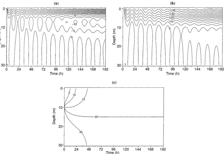
direct simulation consists in modelling the development of inertial oscillations in the presence of a halocline break. An 8-day simulation is performed with a time step of 20 min and a vertical grid size of 2 m. The model is started from a state of rest considering a simpli®ed two-layer water column with fresh water (10 m thick, 0 psu) upon salty water (20 m thick, 30 psu). The wind blows along the x direction and its speed increases linearly from 5 m sÿ1 _{to 10 m s}ÿ1 _{during the simulation.}

The solution of the computation is given in Fig. 1. Inertial oscillations remain trapped in the upper layer of the water column until the mechanical mixing energy, resulting from the downward di€usion of a fraction of the energy input by wind, overcomes the stabilizing e€ect of the strati®cation. Then, the halocline is suddenly broken and the motion can di€use downward and the salinity upward. In the following, these simu-lated data are used as observations to be assimisimu-lated by the optimal control method. An initial model solution (Fig. 2) from which to start the minimizing procedure is computed with a constant value of 10 cm2sÿ1arbitrarily chosen for the turbulent viscosity. One can remark that this value is not accounted for as a ®rst guess in the cost function as it is needed for a weak constraint formula-tion (Eknes and Evensen, 1997) to ensure a single solution (Bennett and Miller, 1991). In a strong constraint formulation, even though it can be used to

accelerate the convergence of the method (Yu and O'Brien, 1991), it is not required if the problem remains over-determined (Menke, 1984). In any case, such a ®rst guess choice could be dicult in this case of time-dependent viscosity.

A comparison between the observation simulation (Fig. 1) and the initial simulation (Fig. 2) shows that the solution of the model is highly controlled by the turbulent viscosity. This latter is about zero at the halocline that acts as a physical wall for the di€usion. As the wind speed increases, the eddy viscosity increases to a threshold value inducing the sudden halocline break. The oscillation amplitude and damping rate follow this time-dependence of the viscosity. As this viscosity varies in the whole space and time domain X …0;s†, the

dimension of the control vector is equal to M N where M is the number of grid points and N is the number of time steps. In order to keep the problem over-determined, the number of data to be assimilated must overtake the control dimension. All the model solution variables, here u;v;S can be taken as observa-tions. Di€erent numerical experiments using di€erent data sets are performed. The variances of the selected data are then set to a ®nite value corresponding to the inverse weights given to each observation. The other data variances are set to in®nity expressing the complete lack of any other available information. The forcing

Fig. 1a±d. Solution of the direct simulation used to construct the observations.aVelocityucmsÿ1

†,bvelocityvcmsÿ1

†,csalinity (psu),d

terms which appear in the second members of Eqs. (25)± (31) are then all equal to zero except for those corresponding to the chosen observations.

3.2 Optimization results

The most basic numerical experiment is to consider all the assimilated data u;v;S as error free data. In comparison with a cost function formulation including a ®rst guess (Yu and O'Brien, 1991), the decrease of the cost functionJis slower, but after about 3000 iterations, J reaches almost zero. The optimized viscosity values (Fig. 3) provide ®elds of u;v;S which appear to be indistinguishable from the observations. This results shows the feasibility of the method without using a ®rst guess. Nevertheless, it must be recalled that such a good ®t between model solution and data set is possible only because the data set was obtained via the completek‡L model and so is fully consistent with the optimization constraints. This cannot be expected with in-situ exper-imental data.

Besides, the optimal set of turbulent viscosity values (Fig. 3) is sometimes di€erent locally from the one given by thek‡Lmodel used to construct the data set. It can be noticed that, even when di€erent, the turbulent viscosity issued from the physical turbulence model and

the optimal viscosity issued from the data assimilation ®tting can lead to the same numerical solution of the model. This paradoxical behaviour can be explained. The optimal viscosity has a degree of freedom (DoF) per grid point and time set whilemt, computed with thek‡L

model, has a smaller number of DoF equal to the number of constants appearing in the k‡L turbulence model. In the optimization procedure, the turbulent viscosity value at a grid point and time step is not

Fig. 2a±c. Solution of the initial simulation with a constant turbulent viscosity mtˆ10 cm2 sÿ1†. a Velocity u…cmsÿ1†, b velocity

v…cmsÿ1_{†,csalinity (psu). The contour intervals are 5 units for each variable plotted}

Fig. 3. Optimal turbulent viscosity…cm2 _sÿ1_{†. The contour}

constrained by the global physical consistency due to the equation of the k‡L turbulence model. Furthermore, the sensitivity of a model to its parametrization may be so weak that the control of these parameters cannot be ensured. As already explained by Panchang and Rich-ardson (1993), the eddy viscosity appear only in the local di€usion terms so that in weak vertical gradient regions, it can take any value without in¯uencing the simulation results. This states the problem of the possibility to control models by parameters that do not have every-where a real in¯uence on the solution.

The ability of the method to recover the model control from a part of the observation data set must now be tested. In a second experiment, where only one variable, for instanceS, is assimilated, the optimization procedure succeeded in recovering exactly the salinity ®eld…J ˆ 0†and the velocity ®elds (Fig. 4) with a better accuracy in strati®ed regions. The controllability prob-lem leads to an optimal eddy viscosity that can take any possible value in zones of zero vertical salinity gradient. The uniqueness of the solution is then not ensured and the turbulent viscosity remains near its initial value …here 10 cm2_sÿ1_{†. For practical purposes, the velocity}

®eld is then a€ected in these regions and it could be worse with another initial value like 0 cm2sÿ1or 100 cm2sÿ1. The retrieval of the velocity

®eld from the salinity ®eld is interesting in itself since hydrological data are often more easily available than dynamic data. It must however be borne in mind that in the model the salt di€usivity is assumed to be propor-tional to the turbulent viscosity for the momentum di€usion (Sc is a constant). Further generalization to models with eddy viscosity and di€usivity using other relationships should be made.

For the same reason, the assimilation of only one velocity componentuorvleads to similar conclusions.u andvare in quadrature, and so give the same content of information for the optimization. The sudden event of the halocline break is included in the velocity ®eld information. In fact, with a slower convergence rate compared with the previous experiment, the model solution is recovered even for the salinity.

The three previous numerical experiments were performed with a great number of DoF with good eciency due to the ideal consistency of the data with the model. Unfortunately, oceanic observations are often sparse and noisy. In order to have a more realistic representation of in-situ observations, the following assimilation experiments are carried out with noisy and sparse data. To simulate di€erent station measurements conducted from an oceanographic ves-sel, either hydrological or current pro®ling

experi-Fig. 4a±d. Optimal solution and optimal turbulent viscosity obtained by the assimilation of the salinity data.aVelocityucmsÿ1

†,bvelocity

ments, the proposed application consists in assimilating noisy velocity and salinity pro®les taken at 48 h, 96 h, 144 h and 192 h. A white and gaussian noise is added with a rms equal to 6 cm sÿ1 _{for the velocities and}

4 psu for the salinity. This rather severe noise has been chosen to test the robustness of the optimal control method. As the control dimension greatly oversizes the number of sparse data, the unique determination of an optimal time-dependent eddy viscosity cannot be expected. To keep the problem over-determined, the control dimension must be reduced at least to the same order as the number of data. Following the idea of Panchang and Richardson (1993), a penalty term …e.g. @mt…t†=@t† could be added in the cost function to

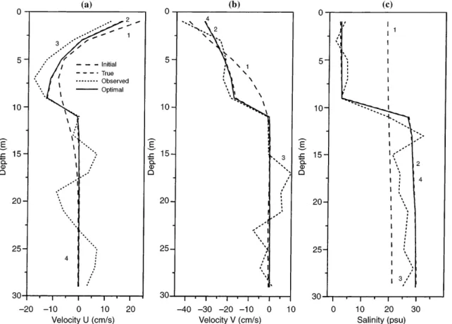
keep a continuous time-dependence of the viscosity. Here, a time-constant turbulent viscosity pro®le over each 48-h time-interval is chosen. The problem consists then in optimizing four viscosity pro®les given for each period: 0 h±48 h, 48 h±96 h, 96 h±144 h, and 144 h±192 h. The pro®le assimilation leads to the recovery of the full solution u;v;S…z;t† (Fig. 5). One can note the time jumps of the solution corresponding to the optimal turbulent viscosity pro®les. Figures 6 shows the u;v;S optimal pro®les att_ˆ96 h (the other time step results are not shown). Even if the assimilated pro®les are noisy, the optimal pro®les are very close to the true pro®les issued from the full solution given by k‡L model. The initial starting pro®les are computed with a

constant viscosity value …10 cm2_sÿ1_{†. Even with severe}

noise, the model is able to extract the mean informa-tion and to supply results provided with some physical consistency given by the model equations. The optimal eddy viscosity pro®les (Fig. 7) evolve with time and with the wind increase. It is almost zero on the halocline for the two ®rst pro®les (48 h, 96 h) before it breaks. When the turbulent viscosity does not control the solution, its value remains near its initial starting value. The non-sequential nature of the proposed assimilation scheme must be underlined. Indeed, the information over the entire data recording is used as a whole to optimize the turbulent viscosity value at a grid point and time step. A sequential optimization would conversely consist in the separate processing of juxtaposed time periods with initial and ®nal state observations. In the actual method, observations on past and future states are accounted for in addition to the initial and ®nal states of the considered sequence. The case of a wrong data pro®le at a given time, say at 48 h, which exhibits for instance a poor vertical resolution leading to an anticipated halocline break, could be corrected with later pro®les where this discontinuity remains.

To summarise the previously described numerical experiment, it can be said that the assimilation technique turns out to o€er a satisfactory robustness with noisy and sparse synthetic data.

Fig. 5a±c. Optimal solution obtained by the assimilation of sequential and noised data (48 h, 96 h, 144 h and 192 h).aVelocityucmsÿ1 †,b

velocityv…cm sÿ1

4 A two space dimension optimization case

The aim of this experiment is to show that the optimal control method can be used for more than one space dimension. The method described in Sect. 2.3 in the more general case has been applied in the previous section for only one space dimension and the time dimension. The control size was already very large in this previous simple case, involving a high numerical cost and a slow convergence of the method. This cost is enhanced by the need of the direct solution to solve the adjoint model: the values of the direct variables are to be stored in the direct path and read from the memory in the inverse path. This is why the control is here limited only to two space dimensions and considered as constant in time. In fact, a space dimension takes the place of the time dimension. For the same reason, a simpli®ed theoretical model of ocean and of wind patterns are considered using a simple geometrical grid. The integration proceeds also for a relatively short simulation time. In addition it is the temperature distribution that here modi®es the strati®cation.

The 2-D space-dependent viscosity optimization problem is exempli®ed on the simulation of a transient coastal upwelling assuming thatmt is time-independent.

The domain is closed to the west by a coast on which zero cross-shore transport conditions are speci®ed. A

Fig. 6a±c. Velocityua, velocityvband salinitycpro®les attˆ48 h.

1, Pro®les from the initial simulation computed with a constant turbulent viscositymtˆ10 cm2 sÿ1†.2, True pro®les.3, Assimilated

pro®les, the true pro®les are noisy. 4, Optimal pro®les, almost superimposed on the true ones

Fig. 7. Turbulent viscosity pro®les.1, Initial pro®le; Optimal pro®les

constant wind…5 m sÿ1_{†is assumed to blow towards the}

north. By assuming the domain is open to the south and to the north, the solution does not vary along the direction y. By taking Neumann open ocean boundary conditions to the south and north, a two space dimen-sion problem in a plane perpendicular to the coast is obtained. Neumann conditions are also imposed at the east boundary. The domain is extended to 40 km from the coast with a horizontal grid sizeDxˆ 2 km, whereas the depth is constant (40 m) with a vertical grid size Dz ˆ 2 m. The latitude is 45N, which leads to a Coriolis parameter f ˆ 10ÿ4sÿ1. The time step is Dt ˆ 50 s for a 48 h simulation. The model is started from a state of rest, a surface temperature of 25_{C and a}

linear vertical gradient of temperature DT

Dz ˆ0:5C mÿ1.

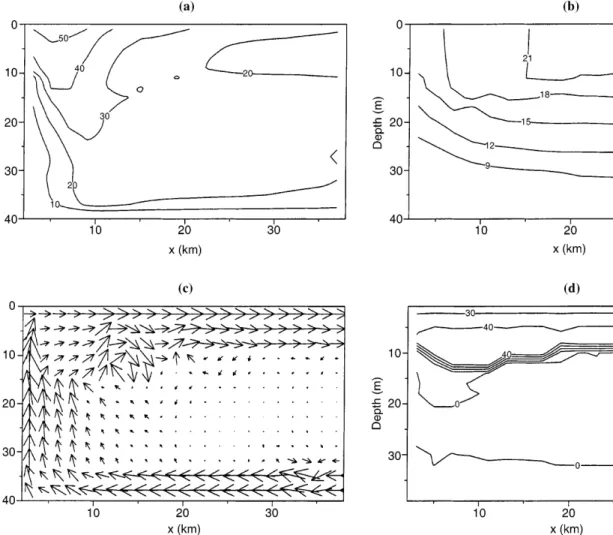
Salinity is taken to be uniform and constant in time. The observations are created from a 2-D steady viscosity ®eld corresponding to the results given by the k_‡L model at t_ˆ48 h. At this time, the turbulent viscosity ®eld is nearly steady and so can be taken as the steady control to be recovered. Nevertheless, one can remark that, even if the viscosity is considered as constant in time, coastal upwelling phenomena is already not steady after 48 h. During this transitional

period, inertial waves always propagate (see Crepon and Richez, 1982, or Kundu et al., 1983, for more details). The model therefore gives results as expected (e.g. Foo, 1981). Close to the coast, nearly 5 km, a coastal jet expands in the direction of the wind. The surface mixing layer is advected towards the open sea, whereas the return current stays between the boundaries of the bottom mixing layer. Near the coast, cold waters are advected from the bottom to the surface. Figure 8 presents the solution …u;v;w;T;mt† at the end of the

observations simulation.

The aim is then to reconstruct the 2D space-depen-dent turbulent viscosity ®eld from the solution of the model. The initial conditions (state of rest and linear temperature strati®cation) are presumed to be known. The initial solution obtained with an uniform viscosity value of 10 cm2_sÿ1 _{(Fig. 9) is considered as the starting}

point of the optimization procedure. The results ob-tained for this initial simulation show that it is necessary to consider a spatial variability of the viscosity.

In order to elaborate the problem and make the method more adapted to usual practical oceanographic application, only temperature data are assimilated, assuming the velocity ®eld to be unknown. As the

Fig. 8a±d. Solution of the direct simulation used to construct the observation of coastal upwelling attˆ48 h:x(km) is the distance to the coast. a Velocity v…cm sÿ1

†, b Temperature C), c vertical

current vector~Uˆ …u;w103_{†, the maximum length is 19 cm s}ÿ1_,d

control is considered as constant in time, a single time sequence of data is needed.

First, it has been chosen to assimilate the complete and noise-free temperature ®eld attˆ48 h. The number of data is almost equal to the number of parameters and it is already a signi®cant diculty to suppose that no information is known for the velocity ®eld and that no other data are available between 0 h and 48 h.

The optimal control method provides by inversion a viscosity ®eld which leads to a quite accurate simulation of the temperature ®eld. One can remark that, as well as with the salinity data in the previous example, the only assimilation of the temperature data allows to recon-struct the dynamics. Figure 10 presents this complete solution, very close to the simulated observations.

Secondly, in order to test the robustness of the method, the previous experiment is realised assimilating the complete but noise-distributed temperature ®eld at tˆ48 h. A white and gaussian noise is added to the temperature ®eld. The level of noise is raised step by step as long as the method remains ecient enough. The deduced borderline case, presented here, corresponds to a noise with a rms equal to 2C, which is more higher than the in-situ measurement errors occurring with

usual devices, such as CTD pro®lers. Figure 11 shows the assimilated temperature ®eld.

It can be seen that the added noise is smoothed by the physics of the model which acts as a strong constraint. The discrepancies of the data with the model, induced by a gaussian and white noise, remains weak enough to allow the method to work as shown in Fig. 12. This 2-D optimization case will allow us to consider more complex situations in the future.

5 Summary and conclusions

As an alternative to classical turbulence modelling, the data assimilation method of optimal control is formu-lated to optimize the turbulent viscosity in a 3-D primitive equation model of the ocean circulation. The chosen model and its full turbulence formulation…k‡L† is described and used to simulate synthetic observations (velocity, salinity or temperature) of two wind-driven events: the ®rst concerns an open strati®ed ocean, and the second, a coastal upwelling. These data are assim-ilated to reconstruct the turbulent viscosity ®eld, which depends either on time and 1-D space or 2-D space. An

Fig. 9a±c. Solution of the initial simulation of a coastal upwelling with a constant turbulent viscositymtˆ10 cm2 sÿ1†attˆ48 h:x(km) is

adjoint model of the direct model (without the complete turbulence formulation) is integrated backward in time to compute the gradient of the cost function with respect to the control and therefore performs the minimization.

The interest of ®tting the vertical turbulent mixing via mt must be stressed. In many coupled

physico-biogeochemical models (e.g. Pinazo et al., 1996), the turbulent state input is only described by a distribution of the eddy vertical viscosity. Its optimization by data assimilation could be useful in this case, the detailed understanding of the turbulent processes not being required. Of course, the success of the method is conditioned by the nature of the data. In the current work, it is pointed out that a vertical mixing process can be recovered using only salinity or temperature data. Furthermore, it would also be interesting to apply this method to reconstruct a physical mixing event from the observations of a conservative tracer (Vandenberghe, 1992).

The optimal control method has shown its eciency in reconstructing the turbulent viscosity ®eld from synthetic velocity or salinity data. Next, as has already been done on a time-independent 1-D optimization in an Ekman model (Yu and O'Brien, 1991), the optimization in a 3-D primitive equation model will have to be tested with assimilation of real observations. This preliminary study has pointed out the diculties that could be encountered.

Fig. 10a±d. Optimal solution and optimal turbulent viscosity ob-tained by the assimilation of the temperature data of the coastal upwelling.x(km) is the distance to the coast.aVelocityv…cmsÿ1

†,b

Temperature (C), c vertical current vector U~ˆ …u;w103_{†, the}

maximum length is 14 cm sÿ1_{,dturbulent viscosity} …cm2

sÿ1 †

The ®rst problem is the large dimension of the control vector. This involves an important numerical cost and a slow convergence rate of the method. Then, a number of data oversizing the control dimension is required. The eddy viscosity variations should be chosen versus the available data. For example, in Sect. 4, as only initial and ®nal states are known, the eddy viscosity is optimized as a time-constant. The full time-space 4-D variational formalism has been described and should be adapted for each physical situation and assimilable data. The second problem is the controllability problem. Prior knowledge of the distributed turbulent viscosity is sometimes not available, especially for a time and space dependent problem, and the method must be investi-gated without ®rst guess. As the eddy viscosity is not always an in¯uential parameter in the calculations, its uniqueness may not be ensured in some areas. Unique-ness in these zones could be achieved using a ®rst guess but with a loss of accuracy of the model results in the strong eddy viscosity in¯uenced regions. Moreover, the optimal viscosity can then take any values which appear sometimes to be physically inconsistent. In the optimi-zation procedure the zero order turbulence closure model allows a degree of freedom by grid point and

time step. In contrast, in thek‡Lturbulence model, the viscosity is strongly constrained by thek and Lvia Eq. (10), and so has a smaller number of degrees of freedom equal to the number of constants …e.g. Cm;k;a;e0†. In

this case, turbulence model calibration is required. It could be viewed as a challenging problem to consider in turn these parameters as controls of the model to be optimized. However, hardly any diculties are probably to be expected due to the strong non linearities of the dependence between the model solution and these constants.

Acknowledgements. Topical Editor D. Y. Webb thanks A. Ochlies and another referee for their help in evaluating this paper.

References

Andre, J. C., G. De Moor, P. Lacarrere, G. Therry and R. Du Vachat, Clipping approximation and inhomogeneous turbu-lence simulations in, Turbulent shear ¯ows I, Springer, Berlin Heidelberg New York, 307±318, 1979.

Begis, D., and M. Crepon,On the generation of currents by winds: an identi®cation method to determine oceanic parameters,

Lecture notes in Physics,58,1975.

Fig. 12a±d. Optimal solution and optimal turbulent viscosity ob-tained by the assimilation of the noisy temperature data of the coastal upwelling.x(km) is the distance to the coast.aVelocityvcmsÿ1

†,b

Blackadar, A. K.,The vertical distribution of wind and turbulent exchange in a neutral atmosphere,J. Geophys. Res.,4,333± 355, 1962.

Blumberg, A. F., and D. M. GoodrichModelling of wind-induced destrati®cation in Chesapeake Bay, Estuaries, 13(3) 236±249, 1990.

Bennett, A. F., Inverse methods in physical oceanography, Cam-bridge University Press, CamCam-bridge, UK, 346 pp, 1992.

Bennett, A. F. and R. N. Miller, Weighting initial conditions in variational assimilation schemes, Mon. Weather Rev., 119,

1098±1102, 1991.

CreÂpon, M. and C. Richez,Transient upwelling generated by two-dimensional atmospheric forcing and variability in the coastline,

J. Phys. Oceanogr.,12,1437±1456, 1982.

Courtier, P., and O. Talagrand, Variational assimilation of meteorological observations with the direct and adjoint shal-low-water equations,Tellus,42A,531±549, 1990.

Devenon, J. L., Optimal control theory applied to an objective analysis of a tidal current mapping by HF radar, J. Atmos. Ocean. Tech.,7,269±284, 1990.

Eknes, M., and G. Evensen,Parameter estimation solving a weak constraint variational formulation for an Ekman model,

J. Geophys. Res.,102(C6),12: 479±491, 1997.

Foo E. C.,A two-dimensional diabatic isopycnal model simulating the coastal upwelling front, J. Phys. Oceanogr., 11, 604±626, 1981.

Gilbert, J. C., and C. Lemarechal, Some numerical experiments with variable-storage quasi-Newton algorithms, Math. Progr.,

45, 407±435, 1989.

Kundu, P. K., S. Y. Chao, and J. P. McCreary,Transient coastal currents and inertio-gravity waves, Deep-Sea Res., 30, 10A: 1059±1082, 1983.

Le Dimet, F.-X, and O. Talagrand, Variational algorithms for analysis and assimilation of meteorological observations: the-oretical aspects,Tellus,38A,97±110, 1986.

Leendertse, J. J., and S.-K. Liu, A three-dimensional model for estuaries and coastal seas: turbulent energy computation,The RAND Corporation (California),Internal Rep., 1977.

Leendertse, J. J., R. C. Alexander and S.-K. Liu, A three-dimensional model for estuaries and coastal seas: principles of computation, The RAND Corporation (California), Internal Rep., 1973.

Lellouche, J. M.,MeÂthodes numeÂriques d'assimilation de donneÂes appliqueÂes aÁ la modeÂlisation tridimensionnelle des eÂcoulements en milieu peu profond, PhD Thesis, Universite d'Aix-Marseille II, 162 pp, 1995.

Lellouche, J. M., J. L., Devenon, and I., Dekeyser, Boundary control on Burgers' equation A numerical approach,Comput. Math. Applic.,28,5: 33±44, 1994.

Lellouche, J. M., J. L. Devenon and I. Dekeyser,Data assimilation by optimal control in a 3-D coastal oceanic model: the problem of the discretization,J. Atmos. Ocean. Tech., 15,2: 470±481, 1998.

Leredde, Y., MeÂthode d'assimilation de donneÂes par contr^ole optimal appliqueÂe aÁ l'estimation des parameÁtres de di€usion turbulente dans un modeÁle 3D de circulation oceÂanique, PhD Thesis, Universite d'Aix-Marseille II, 149 pp, 1999.

Leredde, Y., J. M. Lellouche, J. L. Devenon and I. Dekeyser,On initial, boundary conditions and viscosity coecient control for

Burgers' equation., Int. J. Num. Meth. Fluids, 28, 113±128, 1998.

Lions, J. L.,Optimal control of system governed by partial di€erential equations, Springer, Berlin Heidelberg New York, 396 pp, 1971

Luyten, P. J., E. Deleersnijder, J. Ozer and K. G. Ruddick,

Presentation of a family of turbulence closure models for strati®ed shallow water ¯ows and preliminary application to the Rhine Out¯ow region,Cont. Shelf Res.,16,1: 101±130, 1996.

Mellor, G. L., and T. Yamada,A hierarchy of turbulence closure models for planetary boundary layers,J. Atmos. Sci.,31,1791± 1806, 1974.

Mellor, G. L., and T. Yamada, Development of a turbulence closure model for geophysical ¯uid problems, Rev. Geophys. Space. Phys.,20,851±875, 1982.

Menke, W., Geophysical data analysis: discrete inverse theory.

Academic Press, London, 260 pp, 1984.

Moore, A. M., Data assimilation in a quasi-geostrophic open-ocean model of the Gulf Stream region using the adjoint method,J. Phys. Oceanogr.,21,398±427, 1991.

Munk, W. H., and E. R. Anderson, Notes on a theory for a thermocline,J. Mar. Res.,7,276±295, 1948.

Nihoul, J. C. J., ModeÁles MatheÂmatiques et dynamique de l'environnement, ELE, LieÁge, 198pp, 1977.

Nihoul, J. C. J., E. Deleersnijder and S. Djenidi, Modelling the general circulation of shelf seas by 3Dk_ÿemodels,Earth-Sci.

Rev.,26,163±189, 1989.

Panchang, V. G., and J. E. Richardson,Inverse adjoint estimation of eddy viscosity for coastal ¯ow models,J. Hydraulic Eng.,

119,4: 506±524, 1993.

Pedlosky, J.,Geophysical ¯uid dynamics,Springer, Berlin Heidel-berg New York, 624 pp., 1982.

Pinazo, C., P. Marsaleix, B. Millet, C. Estournel and R. VeÂhil,

Spatial and temporal variability of phytoplankton biomass in upwelling areas of the northwestern Mediterranean: a coupled physical and biogeochimical modelling approach,J. Mar. Syst.,

7,161±191, 1996.

Rodi, W.,Turbulence models and their applications in hydraulics. A state of are review. International Association for Hydraulics Research, Delft, Netherlands, 104 pp, 1980.

Roquet, H., S. Planton and P. Gaspar, Determination of ocean surface heat ¯uxes by a variational method,J. Geophys. Res.,

98(C6),10: 211±221, 1993.

Seiler, U.,Estimation of open boundary conditions with the adjoint method,J. Geophys. Res.,98,C12: 22, 855±22, 870, 1993.

Thouvenin, B., and J. C. Salomon, ModeÁle tridimensionnel de circulation et de dispersion en zone c^otieÁre aÁ mareÂe. Premiers essais: cas scheÂmatiques et baie de Seine,Oceanol. Acta, 7(4),

417±429, 1984.

Van Dam, G. C., and R. A. Louwersheimer,A three-dimensional transport model for dissolved and suspended matter in estuaries and coastal seas, inDynamics and exchanges in estuaries and the

coastal zone, Coastal and Estuarine Studies 40 A.G.U.

Washington, DC, pp. 481±506 Ed., D. Prandle 1992.

Vandenberghe, F., Assimilation de measures satellitaires dans les modeÁles numeÂriques par meÂthodes de contr^ole optimal, PhD Thesis, ENSM Paris, 1992.