Abstract— A modified edge detection algorithm has been presented here that uses logarithmic transform and Hyperbolic Tangent (HBT) filter. The proposed algorithm incorporates Logarithmic transform along with Luminance and Contrast-Invariant Edge Similarity Measure algorithm for edge detection. The proposed algorithm gives a good quality edge detection of images with improved SSIM value and almost equal or higher PSNR values.
Index Terms— Edge-Detection, HBT filter, Logarithmic Transform, Structural Similarity, Similarity Measure.
I. INTRODUCTION
Accurate detection of edges is not possible most of the times due to contrast and noise sensitivity, and uneven illumination. Classical Gradient-Magnitude (GM) methods for edge detection [3] depend on edge strength and they usually do not detect weaker edges. Angle-based (AN) methods, which are based on the computation of the cosine of the projection angles between neighborhoods and predefined edge filters, can be used for detecting valid edges regardless of their magnitude, , but they are sensitive to noise and uneven illumination [5]. Same problem is faced by local thresholding of images because they tend to inhibit edges in regions of low luminance.
Smoothing as a pre-processing step is required by optimal step-edge detectors such as Canny’s Gaussian first derivative (GFD) [3] filter to reduce noise. This smoothing process makes weak edges harder to detect. A method proposed by Kovesi [4] represents images in the frequency domain and edges correspond to the points of maximum phase congruency. Phase Congruency (PC) methods are invariant to contrast and illumination changes, but gives poor edge localization.
An edge detection algorithm has been proposed by Saravana Kumar et al. [1] that give better result than GM and AN method. Their method gives better edge localization and is more robust in the presence of varying illumination, contrast and noise level. It is based on edge similarity measure between image neighborhoods and directional finite impulse response (FIR) with hyperbolic tangent (HBT) profiles.
Madhu S. Nair is with the Department of Computer Science, Rajagiri College of Social Sciences, Kalamassery, Kochi – 683104, Kerala, INDIA.(e-mail: [email protected]).
R. Vrinthavani is with Defense Research and Development Organization (DRDO), Bangalore, INDIA. (e-mail: [email protected])
Dr. M. Wilscy is with the Department of Computer Science, University of Kerala, Kariavattom, Trivandrum 695 581, Kerala, INDIA.(e-mail: [email protected]).
Drawback of this method is that the final edge-detected images do not have enough structural similarity with the original image.
This paper proposes a modified edge detection algorithm that uses HBT filter and Logarithmic transform that preserves structural similarity with the original image and gives better edge detection. Consequently, a better Structural Similarity Index (SSIM) can be achieved compared to the conventional edge detection techniques as well as the edge detection based on edge similarity measure. Compared to the edge detection using similarity measure, the Peak Signal-to-Noise ratio (PSNR) will be almost equal or higher for the proposed method. A drawback of the proposed method compared to edge similarity measure algorithm is that latter gives a better edge detection in the case of contrast variant and noisy images. But still the proposed method gives an acceptable result in the case of noisy and contrast variant images. Smoothening as a preprocessing step can be applied in the case of noisy images to get better edge-detection and yield higher structural similarity. The proposed algorithm gives better results for noiseless and luminance variant images.
II. EDGE DETECTION USING HBTFILTER
The edge detection method using similarity measure proposed by Sarvana Kumar et al. [1] obtains an optimal estimate of image edges by using principal component analysis (PCA). PCA is applied to a set of local neighborhoods bi of size n × n to generate n2 eigenvectors
}
1
,
{
e
i≤
i
≤
n
2 each of size n × n. A neighborhood bi can beexpressed as
bi =
∑
=
+
21
n
j j ij
e
u
m
,where the average over all local neighborhoods is
m =
∑
=
N
i i
b
N
11
and uij is the projection of bi –m onto the j th
eigenvector ej.
The eigenvector pair has similar profiles but is orthogonal. The number of zero crossings in the eigenvectors increases from eigenvector pair e2 - e3 to e6 - e7 and beyond, indicating that the eigenvectors corresponding to smaller values of Eigen values capture higher frequency information of the local neighborhoods and, hence, are more susceptible to noise. Two eigenvectors e2 and e3 are considered for edge detection since they most accurately approximate the gray-level variation in local neighborhoods. Since e2 and e3 have blurred
HBT Filter and Logarithmic Transform Based
Edge Detection – A Modified Approach
The region of support for GW is limited by window size W to
ensure edge localization.
The FIR filter pair h1 and h2, is obtained by sampling GW at
integer locations (xd, yd) within [-W, W]. The weights αij are
determined by projecting both e2 and e3 onto h1 and h2, i.e. j
j j i
ij
=
e
,
h
h
,
h
α
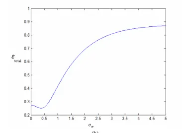
. The parameter σW defines thesteepness of the profile at zero crossing and its relationship to filter support. σW for a given filter width W is determined
such that the HBT filter pair can best approximate the natural step edges in an image. This is done by selecting σW for a
given W such that its corresponding total approximation error is minimized. The approximation error is given as
j j i
i
=
e
−
e
ˆ
e
ε
and the total approximation error is given asε
total=
ε
2+
ε
3. The edge detection using edgesimilarity measure uses cosine measure Ri with regularization
parameter γ and an empirically determined constant c. It is given by,
g
c
b
b
g
c
b
b
R
i i i i i.
,
γ
γ
+
−
+
−
=
An estimate
γ
ˆ
of regularization parameter γ is given by6745
.
0
)
1
:
(
ˆ
=
median
Y
i≤
i
≤
N
γ
,where
∑
=
−
=
2 1 22
[
(
)
]
1
nj
i i
i
b
j
b
n
Y
i=1,2,….,N. III. LOGARITHMIC TRANSFORM DOMAIN
The logarithmic transform domain [2] affords us the ability to view the frequency content of an image. The transformation is applied to the image in the frequency domain. This is done in two steps. The first step requires the creation of a matrix to preserve the phase of the transformed image. This will be used to restore the phase of the transform coefficients. The next step is to take the logarithm of the modulus of the transform coefficients as follows:
)
)
,
(
ln(
)
,
(
ˆ
i
j
=
X
i
j
+
λ
X
where
λ
is some shifting coefficient. The shifting coefficient is used to keep from running into discontinuities. To return the coefficients to the standard transform domain, the signal is exponentiated and the phase is restored. This approach can be extended by using the following operator/function:applied to the image in frequency domain that attenuates low frequency components. The details of the modified edge-detection method are as follows:
Step 1: Apply the Fourier transform to the given image f. The Fourier transform of an image is given as
=
∑ ∑
− = − = + − 1 0 1 0 ) / / ( 2)
,
(
1
)
,
(
M x N y N vy M ux je
y
x
f
MN
v
u
F
ππππStep 2: Compute the Fourier spectrum and the phase angle of the Fourier transform. The Fourier spectrum
)
,
(
u
v
F
and the phase angleφφφφ
(
u
,
v
)
of the Fourier transform is given as[
2 2]
1/2)
,
(
)
,
(
)
,
(
u
v
R
u
v
I
u
v
F
=
+
=
−)
,
(
)
,
(
tan
)
,
(
1v
u
R
v
u
I
v
u
φφφφ
where R(u, v) and I(u, v) are the real and the imaginary parts of F(u, v), respectively.
Step 3: Apply the logarithmic transform to the Fourier spectrum,
F
(
u
,
v
)
. The logarithmic transform domain [2] affords us the ability to view the frequency content of an image. The transformation is applied to the image in the frequency domain. This is done in two steps. The first step requires the creation of a matrix to preserve the phase of the transformed image. This will be used to restore the phase of the transform coefficients. The next step is to take the logarithm of the modulus of the transform coefficients as follows)
)
,
(
ln(
)
,
(
ˆ
u
v
=
γγγγ
ηηηη
F
u
v
+
λλλλ
F
where γγγγ, ηηηη and λλλλ are parameters, that are computed empirically.
Step 4: Apply the luminance and contrast invariant edge similarity measure algorithm to
F
ˆ
to get the similarity mapR
ˆ
.Step 5: Apply the inverse logarithmic transform of
R
ˆ
. Inverse logarithmic transform is done as follows)
/
)
)
/
ˆ
(exp(
)
,
(
=
γγγγ
−
λλλλ
ηηηη
′
u
v
R
R
) , ()
,
(
)
,
(
u
v
R
u
v
e
j uvR
=
′
⋅
φφφφThen apply the inverse Fourier transform on
R
(
u
,
v
)
to get R(x, y).(a) (b) (c)
Fig 1. Comparison of outputs for lena.tif image. (a) Original Image. (b) Edge-detected image using edge similarity measure. (c) Edge-detected image using proposed method.
(a) (b) (c)
Fig 2. Comparison of outputs for tree.tif image. (a) Original Image. (b) Edge-detected image using edge similarity measure. (c) Edge-detected image using proposed method.
(a) (b) (c)
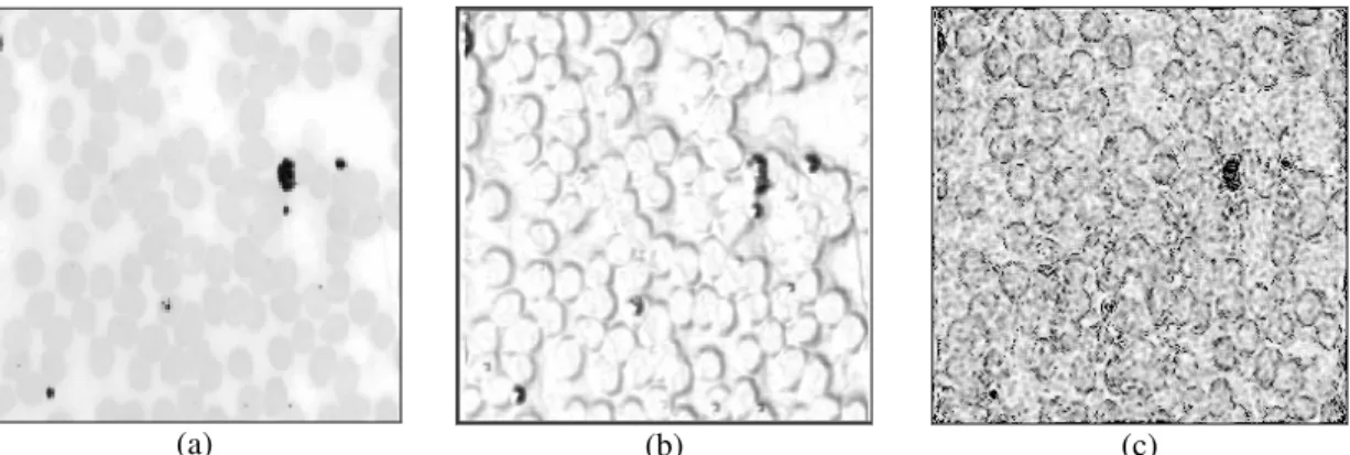
Fig 3. Comparison of outputs for aila.tif image. (a) Original Image. (b) Edge-detected image using edge similarity measure. (c) Edge-detected image using proposed method.
(a) (b) (c)
(a) (b) (c)
Fig 5. Comparison of outputs for coins.png image. (a) Original Image. (b) Edge-detected image using edge similarity measure. (c) Edge-detected image using proposed method.
(a) (b) (c)
Fig 6. Comparison of outputs for rice.png image. (a) Original Image. (b) Edge-detected image using edge similarity measure. (c) Edge-detected image using proposed method.
(a) (b)
(c) (d)
Fig 7. Least-square estimates of PCA eigenvectors using HBT filters (a) and (b) are PCA Eigen vectors of second and third largest Eigen values in spatial domain for Lena image; (c) and (d) corresponding values in the frequency domain.
(a) (b)
Fig 8. (a) σW values in spatial domain (b) σW value in frequency domain
TABLE I
Comparison of PSNR, SSIM, Luminance (I), Contrast (C) and Structure (S) values
Luminance/Contrast Invariant Edge Similarity
Measure Edge Detection Using HBT Filter and Logarithmic Transform
PSNR SSIM Lum
(I)
Cont (C)
Struc
(S) PSNR SSIM Lum
(I)
Cont (C)
Struc
(S) η γ λ
Rice 5.725 -0.191 0.794 0.999 -0.241 6.344 0.183 0.812 0.961 0.235 1.2 10 2 Lena 5.495 0.02 0.765 0.977 0.027 5.552 0.199 0.764 0.999 0.261 1.2 10 2 Coins 4.898 -0.322 0.789 0.998 -0.409 4.948 0.0013 0.752 0.986 0.002 1.2 10 1.5
Aila 6.402 0.047 0.802 0.962 0.0615 6.872 0.167 0.807 0.985 0.211 1.2 10 2 Cell 16.623 0.086 0.999 0.788 0.108 19.424 0.307 0.999 0.927 0.331 1.2 10 2 tree 6.932 .011 0.84 0.888 0.014 8.3 0.277 0.872 0.964 0.33 1.2 10 2
Step 7: Take the complement of the result obtained from the previous step and save it in a variable, say gneg. Step 8: Apply the image adjustment (imadjust) operation to gneg to get the image A with clear edges.
Step 9: Apply the Wiener filter and image adjustment operation (this is an optional step) to A in the case of noisy and contrast variant images to get better result.
V. RESULTS AND DISCUSSION
The similarity feature of the proposed method is compared with luminance and contrast invariant edge similarity measure algorithm [1]. The proposed method was applied to six standard images namely Lena, Tree, Aila, Cell, Coins and Rice shown in fig 1, 2, 3, 4, 5 & 6 respectively. The comparison results are displayed in Table I in terms of SSIM and PSNR values, where Lum, Cont and Struc stands for Luminance, Contrast and Structure, respectively.
It can be seen that PSNR values are almost similar; however, there is remarkable improvement in their SSIM values, especially in its structural component. The tree and cell images are noisy and contrast variant images. In these two
images the ninth step is applied. In all the other images sixth step has been applied. Figure 7 shows the comparison of the second and the third largest eigenvectors of the PCA analysis in the spatial domain and frequency domain. Figure 8 shows the comparison of σW in the spatial and frequency domain.
VI. CONCLUSION
A modified edge detection algorithm has been presented in this paper which gives a better edge-detection while preserving the structural similarity with the original image. Logarithmic transform and HBT filter has been employed in the proposed method for yielding better result. As mentioned earlier, a drawback of this method is that, in the case of contrast variant and noisy images, edge-detection algorithm based on similarity measure gives better result. Our future research will be focusing on how to improve the performance of the proposed method in the case of noisy and contrast variant images.
REFERENCES
[5] W. Frei and C.C. Chen, “Fast Boundary Detection: A Generalization and a New Algorithm,” IEEE Trans. Computers, vol. 26, pp. 988-998, 1977.
[6] R. C. Gonzalez and R. E. Woods, Digital Image Processing, 2nd ed. Englewood Cliffs, NJ: Prentice-Hall, 2002, ISBN: 0-201-18075-8. [7] Anil K. Jain, “Fundamentals of Digital Image Processing”, 1st Ed.,
Prentice Hall, Pearson Education, 1989.
Madhu S. Nair is currently working as Lecturer in the Department of Computer Science, Rajagiri College of Social Sciences, Kochi, Kerala, India. He received his Bachelors degree in Computer Applications (BCA) from Mahatma Gandhi University with First Rank and Masters Degree in Computer Applications (MCA) from Mahatma Gandhi University with First Rank. He also holds a Post Graduate Diploma in Client Server Computing (PGDCSC) from Amrita Institute of Technology. He had also qualified National Eligibility Test (NET) for Lectureship conducted by University Grants Commission (UGC) and Graduate Aptitude Test in Engineering (GATE) conducted by Indian Institute of Technology (IIT). He has published several papers in reputed National and International Journals and Conferences, which includes IEEE, Springer, IAENG, etc. He is a Life Member of Computer Society of India (CSI) and a member of International Association of Engineers (IAENG). His areas of interest include Image Processing, Neural Networks, Computer Networks and Software Engineering.
R. Vrinthavani completed her B.Tech and M.Tech from University of Kerala. Currently she is working as a Scientist, Defense Research and Development Organization (DRDO), Bangalore, India. Her areas of interest include image enhancment, image edge detection, image segmentation etc.