Worker remittances and government behaviour in
the receiving countries
Thomas H.W. ZIESEMER*
Abstract
We estimate the impact of worker remittances on savings, taxes, and public expenditures on education, all as a share of GDP, for two samples of poor and less poor countries. Remittances increase the savings ratio in both samples. Savings have an (inverted) u-shaped impact on the tax ratio in poor (richer) countries. Higher tax revenues lead to higher public expenditure on education in both samples. When remittances increase, in the richer sample, governments raise less tax revenues but spend more on education in direct response, whereas governments of the poorer sample raise more tax revenues at low levels of remittances, but less at high levels of remittances. In simultaneous equation simulations of a positive permanent shock to remittances, the governments of richer countries reduce taxation and public expenditure on education as a share of GDP. In poor countries, this leads to higher tax revenues and spending of more money on education.
Key words: remittances, savings, tax revenues, public expenditure on education
JEL Classification: E21, F24, H20, H52, I22
1. Introduction
The literature on the effects on worker remittances has mainly focused on behaviour of private households, but has said little about the reaction of governments in the receiving countries. For example, in the survey of Lucas (2005),ă theă wordă ‘tax’ă doesă appeară bută alwaysă withoută anyă referencingă toă empirical work. Whereas some countries such as Morocco tax worker remittances heavily and therefore worker remittances should increase tax revenues, it is also possible that growth is increased through remittances and
*Thomas H.W. Ziesemer is professor at the Department of Economics, Maastricht University, and UNU-MERIT, Netherlands; e-mail:[email protected].
therefore the ratio of tax revenues as a share of GDP may go up or down and other countries provide tax incentives to attract remittances (Ratha 2004). In addition, other determinants of taxation like savings may increase as well and therefore remittances may have an indirect effect on taxation via them. 1 Recently, Ziesemer (2008, 2012b) and Ebeke (2010) have treated the impact of remittances on tax revenue. Ziesemer (2008) found that remittances decrease the tax ratio in the richer sample but increase it in the poorer sample. Ebeke (2010) findsă‘thatăremittances significantly increase both the level and the stability of government tax revenue ratio in the receiving countries that have adopted the VAT’ă foră aă sampleă ofă 111ă countries.ă Ziesemeră(2008,ă 2012b)ăfindsă aă positiveă effect for a poor country sample using methods slightly different from the ones we use here.
Similar to the scarcity of findings regarding tax revenues, we do not
find any information about the reaction of public expenditure on
education to the appearance of worker remittances although theoretical
workă usesă ‘theă assumptionă …ă thată theă diasporaă beară theă costsă ofă
education’ă (Weiă andă Balasubramanyam
, 2006, p.1608). This naturally
raises the question whether the government then reduces or increases its
own efforts. As a matter of subjective selection we think that this is a
highly relevant government variable, as it contributes to human capital
formation, which is important for many aspects of economic
development. Recently, Ziesemer (2008) and Ebeke (2012) have treated
the impact of remittances on public expenditure on education. Ziesemer
(2008) found that in the richer sample (above $1200 per capita income)
the total effect of remittances is negative in the short run and almost zero
in the long run and for the poorer sample the total effect of remittances is
positive in the short as well as in the long run. Ebeke (2012) finds a
negative impact of remittances on public expenditure on education for a
sample of 86 countries if governance is bad.
We will therefore focus on the effects of worker remittances on tax revenues and public expenditure on education, all expressed as a share of GDP. We will try to explain empirically the determination of these variables for two sets of countries, one with a per capita income above and the other below $1200 in 2003 in order to figure out how governments of poor and less poor countries react to remittances and other determinants. The poorer sample consists of 52, and the richer sample of 56 countries. For both samples, we have data on worker remittances and development aid and both contain former communist countries.
Of course, with these questions we are no longer in the realm of pure economics but rather also in politics. We will try to find preliminary answers via an estimate of an empirical model for two panels of countries explained in section 2.2 In section 3, we describe the data and the econometric method used. In section 4, we present the results. In section 5, we show baseline simulations and scenarios for permanent shocks to remittances as a share of GDP. Section 6 summarizes and points to issues for further research.
2. An empirical model
Weăspecifyătheăfollowingătaxăfunctionăexplainedăbelowăusingătheăindexă‘i
forăcountriesăandă‘t’ăforătime.ă
taxyit = a0,i + a1taxyit-1 + a2savgdpit + a3(wr/gdp) it + uit (1)
For the explanation of tax revenues as a share of GDP, taxy, the first argument besides a country-specific constant is its lagged value, taxy(-1),
implicitly capturing the history of tax policy. Taxability is well known to be limited by poverty in poor countries; whatever drives government behaviour, the resistance against taxation is larger and more accepted in general when people are poorer. Poverty itself can be expressed in many ways. The literature uses mostly per capita income or expenditure variables followed by a discussion of distribution issues. The idea used here, related to traditional surplus debates, is that the savings ratio, savgdp, reflects how much of their income people can miss in view of the minimum requirements for existence. In rich or less poor countries savings ratios may also reflect how much people can care for themselves rather than relying on state support. The idea for poor countries then would suggest that we get a positive sign for the coefficient of savings, but possibly a negative one for sufficiently less poor countries. We consider worker remittances, wr, as a share of GDP as a sort of marginal income received. The question then is whether governments want to tax this at higher rates in the spirit of progressive taxation or at lower rates, as under special tax incentives intending to attract remittances. A negative sign could also imply that the effect
2Whereasătheăquestionă‘whyădoăgovernmentsăbehaveăasătheyădo’ămightăbenefităfromăaătheoreticală model, we do not need one here because we only want to find in this paper which direction the
on the GDP (the denominator), not discussed explicitly in this paper, is larger than that on taxes (the numerator). We will also explore the use of quadratic terms for all regressors.3 The last term in the regression is the residual. In principle, we might have used per capita income rather than the savings variable. However, it has a growth trend and even when employing quadratic and cubic terms with or without a time trend the tax variable would go out of bounds in all intertemporal simulation exercises we have carried out. We have also tried out literacy as a regressor because it might be a motive for raising taxes, and it is relevant for some development issues, but it has turned out to be insignificant. We did try out the use of natural logarithms besides quadratic and cubic terms for all variables.
Remittances may not only have a direct effect on tax ratios, but also an indirect effect via savings ratios. Remittances add to disposal income and if taxes do not take away the total increase, both consumption and savings will both increase if they are not inferior.4 An interesting question then is whether the
share of consumption or savings are increasing or decreasing.5 For savings ratios
we specify the following regression.
savgdpit = b0,i + b1savgdpit-1 + b2(wr/gdp) it + b3(oda/gdp) it +
+ b4d(log(gdppcit)) + b5log(1+riit-1) + b6 (peegdp)it + b7 (nm/l) it + eit (2)
Again, there is a country-specific constant and a lagged dependent variable. Worker remittances are international transfers received by private households. They enhance disposable income. Households can use remittances as a share of GDP to enhance or reduce savings ratios depending on whether they go more or less than proportionately into consumption or savings (Griffin 1970). Official development aid is an international transfer as well and enhances disposable income of the country, mostly of the government though. This also may provide an incentive to increase or decrease savings ratios and therefore we add it also as a regressor, oda/gdp. The growth rate of the GDP per capita,
3 The effect of remittances on tax revenues can also serve as a channel for shocks from the sending countries as in Ziesemer (2010a) and Abdih et al. (2012).
4 Osili (2007) provides portfolio theory and evidence for the effect of remittances on household savings.
gdppc, and the interest rate, ri, may have an impact as in basic macroeconomic textbooks to the extent that people base their plans on looking into the future. Public expenditure on education, peegdp, may reduce the private incentives to save and reduces government savings directly. Net immigration, nm, taken as a share of the labour force, l, to correct for country size may enhance savings ratios if the immigrants bring high savings with them to the country of arrival. Conversely, emigrants may dis-save because they probably prepare their emigration by saving money to carry the cost of migration. The last term in the regression is the residual.
On the expenditure side, public expenditure on education as a contribution to financing the development of capability or human capital building is one of the much-discussed items in development studies. We specify the following regression.
peegdpit = c0 + c1peegdpit-1 + c2 taxyit + c3savgdp it + c4(wr/gdp) it + c5 (oda/gdp) it
+ it (3)
Besides the constant and the lagged dependent variable, the more tax money is available, the more can go to education. The more people save, the more they signal that the government should do the same concerning education. In addition, education may become accessible in poor countries if private and public money support it, but not if only one of them does so. This would provide an incentive to invest more in education publicly. On the other hand, savings and worker remittances may discourage public expenditure on education, because the government may think that people can take care of themselves more than before. Development aid might encourage public expenditure on education, for example via co-financing between donors and governments. However, it is also possible that more aid on that purpose leads to less public money. Again, the last term is the residual.
There are three channels then along which remittances affect public expenditure on education. First, they have a direct impact. Second, there is an impact via savings, a private channel, and third, there is an impact via the tax ratio, which in turn depends itselfon an effect via savings.6 Private and public behaviour are strongly interwoven here.
3. Data and econometric method
We take all data from the World Development Indicators, World Bank (2007)7, where definitions are given. More detailed information is available from
6 As a matter of cross checking, we did not find an impact of remittances on aid.
the sources mentioned below. Worker remittances are official receipts in constant (2000) US$ and do not contain compensation of residents going across the border to work in neighbouring countries. The data stem from Balance of Payments Statistics.8 Flows going via financial investments and withdrawals from related accounts are not included (see IMF 2005, p.99). Unofficial receipts may be high - Freund and Spatafora (2005) estimate that informal remittances are between 35 and 75 per cent of the official ones - and important but we have no way to deal with the issue directly (see Adams and Page, 2005)9. Taxes are only those of the central government. This is a limitation, but the best-known federal states like the USA and Germany are not in our sample. Savings are gross of depreciation but include net current transfers and net income from abroad. Data on official development aid include loans containing at least a grant element of 25 percent. When taking remittances and aid as a share of GDP, we use algebraic expression where the 3 percent is 0.03. For the other data, taken from the WDI as they are expressed there, shares of GDP are multiplied by 100, and then 3 percent is just three. Data of the GDP per capita, gdppc, are in constant (2000) US$ and stem from national accounts. Interest rates, ri, are real rates as obtained by use of the GDP deflator and taken from the IMF IFS Yearbook. Data on public expenditure on education, peegdp, are from the UNESCO and we assemble them from several versions of the World Development Indicators.10 Data on migration are five-year estimates of the United Nations Population Division. Labour force data are from the ILO. We use available data for remittances and aid for 108 countries. We divide these countries into two groups, those with a GDP per capita that is above and below $1200 in 2003 because Kernel density estimates for the years 1960, 1970, 1980, 1990 and 2000 show peaks at around $1000. The number of countries around this peak is almost constant over time. Analysis of growth rates
(see Ziesemer 2012a). This would also change the N/T ratio. Results are in general dependent on the N/T ratio of panels (Smith and Fuentes 2010) and having different N/T ratios might make comparison across samples impossible in particular for equation (3) with roughly six observations per country and each 29 countries. In this respect the N/T ratios are comparable for equations 1a and b and also 3a and b but hardly so for 2a and b. Adding observations for the richer sample might turn this around implying that updating is devalued by loss in comparability.
8 In the WDI, there are surprisingly many zero values, which are quite implausible because they are preceded and followed by positive values of non-negligible size. We have turned them into
‘non-available’.ă
9 We would like to point out though that GDP data also underestimate economic activity because of the neglect of the informal sector. Schneider and Enste (2000, Table 2) report values of 25-76 percent of GDP for developing countries. This is the same order of magnitude as for remittances. For developed countries, these values are lower. Informal remittances are falling as a share of the official ones. It is not clear though that the share of the informal sector is falling in developing countries over time. The imperfection of remittances data is broadly discussed in all related papers. That of GDP data is not discussed anymore although it may still be as severe.
shows that the countries in the poor group have an average growth rate below 1 percent in the period 1960-2005. Those in the less poor group have growth rates above 2 percent. Another important difference between the two groups is that in the case ofthe richer sample, remittances are a larger share of GDP than aid is, 4 percent and 2 percent respectively. However, for the poorer sample this often-stated result is by far not true. Aid is more than 9 percent and remittances are above 3 percent in the poor sample. Panel homogeneity then is hardly a convincing assumption concerning both the level and the growth rates of the GDP and therefore we split the sample. In the richer sample, we will then have 56 countries and 52 in the poorer one (see Appendix A for the lists of countries). We postpone further splits to future research. Data for the respective variables are not available for all countries and years though and therefore our regressions will often cover less than the 52 or 56 countries. All regressions therefore use unbalanced panel data.
For all equations, we follow a basic econometric lesson for macroeconomic variables, to include the lagged dependent variable. It tends to be highly significant in most circumstances and therefore it is always included in order to avoid an omitted variable bias (see Greene, 2003, Chaps. 19 and 20). By implication, we consider dynamic panels.
Moreover, results in dynamic panels depend on the ratio N/T, where N is the number of cross-sections and T is the number of periods (Smith and Fuentes 2010). As we are dealing with a dynamic issue, we like to have a long time dimension T and therefore we use yearly data rather than five-year averages.
A basic econometric lesson here is that in dynamic panels the coefficient of a lagged dependent variable, when using a fixed effects estimator, has a downward bias of an order of magnitude of 1/T. This is an expected value of the bias for the case of having no further regressors; with more regressors, it is lower (Asteriou and Hall 2011, chap.19). Its standard deviation allows for having a much higher or lower bias. The Anderson-Hsiao estimator removes the bias, but is inefficient. The Arellano-Bond GMM estimator using first-differences of the model has a small sample bias. The best response to this currently is the use of a system GMM estimator by Arellano and Bover (1995) as shown by Monte-Carlo studies by Blundell and Bond (1998) for very small T and by Soto for T=15. It combines the within estimator of the level equation with their version in first differences, imposing equality constraints on the respective coefficients of the regressors. Alternatively, one method of estimation for system GMM is called ‘orthogonalădeviations’;ăităreplacesătheăfirstădifferenceăequationămentionedăaboveă by orthogonal deviations, which consist of a Helmert transformation, i.e. it subtracts from each residual the sum of the future residuals.11 As many
regressors are under suspicion of endogeneity, we use instruments also for some of the regressors other than the lagged dependent variable in this approach. The orthogonal deviation approach does not estimate the intercept of the above equations. Therefore, we will leave the coefficient in its general form when reporting results; alternatively, we could present the estimation results in terms of first differences, which would cost more space though. The GMM approach minimizes a quadratic form called the J-statistic. If the number of instruments used is identical to the number of regressors, the J-statistic is zero. When more instruments are used, the J-statistic increases. It should not increase too much for instruments to be valid according to the chi-square test, but also not too little because then, instruments do nothing or too little. An extremely high (low) Hansen-Sargan p-value (henceforth HS p-value) indicates that it is not increasing too much (little). Roodman (2009b) argues that the p-values should not be too far outside the range of 5 percent and 25 percent. It remains unclear thoughăwhatăisă‘tooăfar’.ăTherefore,ăweăreportătheăJ-statistic, the HS p-value and the standard error of regression whenever we use the Arellano-Bover method.
Blundell and Bond (1998) and Soto (2009) use the assumption of equal unit variances for the fixed effects and the residuals in their Monte Carlo studies. Bun and Windmeijer (2010) have shown that for a ratio of four there is an upward bias of the system GMM estimator of about 9% if T = 6 and of about 7%
if T = 15. As we have T = 10 we could expect a bias of about 8% if the variance
ratio were four. However, it remains unclear in the study by Bun and Windmeijer (2010) what the bias would be when more regressors are employed rather than only the lagged dependent variable. Therefore, it is currently not possible to deal rigorously with this aspect. Similarly, Bazzi and Clemens (2010) deal with the endogeneity of one endogenous regressor in addition to the lagged dependent variable. They show that in addition to the Bun/Windmeijer results, the correlation coefficient between the two residuals of the Monte Carlo model should not be large and the regression coefficient of the regressor and its own lag should be high. Most GMM estimates have more regressors though and it is unclear how serious the problem is in these cases. Moreover, both studies do not deal with the orthogonal deviation method we use here.
Wu-Hausman (DWH) test in the version of Davidson and McKinnon (2004) to test for endogeneity.12 This information together with assumptions on pre-determinedness versus exogeneity is used for the choice of instrumental variables in the Arellano-Bover (1995) orthogonal deviation version of our system GMM estimate; see Appendix B which also reports the results for the difference-in-Sargan test for the use of additional instruments. We compare the coefficient of the lagged dependent variable from the GMM estimate with that from a fixed effects estimate in order to make sure that the bias correction is not larger than 1/T.
4. Results
We present here the regression results first for the countries with aGDP perăcapitaăaboveă$1200ăindicatedăbyăană‘a‘ăinătheăequationănumberăandăthenătheă resultăforătheăcountriesăbelowă$1200ăindicatedăbyăaă‘b’ăinătheăequationănumber.ă We present results first from an econometric perspective in section 4.1 linking back to the discussion in the previous section and then discuss them from an economic perspective in section 4.2.
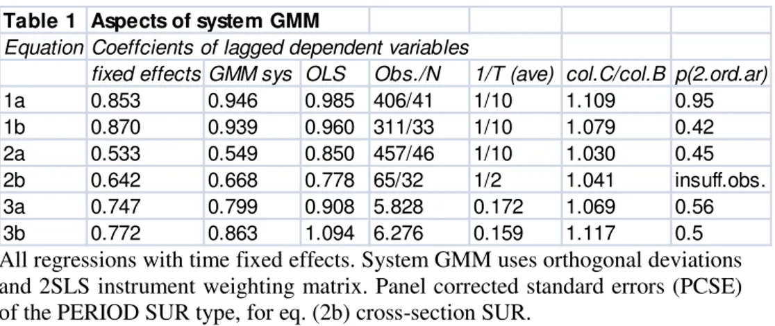
Table 1 Aspects of system GMM
Equation Coeffcients of lagged dependent variables
fixed effects GMM sys OLS Obs./N 1/T (ave) col.C/col.B p(2.ord.ar)
1a 0.853 0.946 0.985 406/41 1/10 1.109 0.95
1b 0.870 0.939 0.960 311/33 1/10 1.079 0.42
2a 0.533 0.549 0.850 457/46 1/10 1.030 0.45
2b 0.642 0.668 0.778 65/32 1/2 1.041 insuff.obs.
3a 0.747 0.799 0.908 5.828 0.172 1.069 0.56
3b 0.772 0.863 1.094 6.276 0.159 1.117 0.5
All regressions with time fixed effects. System GMM uses orthogonal deviations and 2SLS instrument weighting matrix. Panel corrected standard errors (PCSE) of the PERIOD SUR type, for eq. (2b) cross-section SUR.
4.1. Econometric results: Aspects of system GMM estimation
Table 1 shows the coefficients of the lagged dependent variable for fixed effects estimation in column 1, for system GMMestimation in column 2, and for OLS in column 3. In all cases, the value from system GMM is between the under-estimating one from fixed effects and below the over-estimating one from OLS. The number of periods is much larger in all cases than the number of observations divided by the number of countries, as indicated by columns 4 and 5. The expected bias in the column denoted as 1/T is between 10 and 50 percent. The system GMM estimate of the lagged dependent variable should therefore be
10-50 percent higher than that of fixed effects if there were no other regressors. Roughly, in all six equations we find that the correction is equal to 1/T or lower as it should be because there are more regressors than only the lagged dependent variable.13 Finally, second order serial correlation should be absent. We present the p-values for the regression of the first difference of residuals on their own second lag in the last column, indicating the absence of second-order serial correlation (see Roodman 2009a).14
4.2. Economic results: estimation and interpretation
Foră theă sakeă ofă brevity,ă weă abbreviateă theă savingsă ratioă asă ‘s ‘,ă theă
remittanceăratioăasă‘w’,ătheăpeegdpăasă‘p’,ăd(log(gdppc))asă‘g’,ărealăinterestăratesă
asă‘r’,ăandătheădevelopmentăaidăratioăasă‘d’.ăăInăparentheses,ăweăpresentăp-values, the significance levels.15 Appendix B shows the instruments. To save space we do not write down information on time fixed effects and drop the residuals from the equations.
taxyit = a0,i + 0.946taxyit-1 - 0.16sit + 0.004sit2 -20.16(wit-1)2
(1a)
(0.00) (0.09) (0.052) (0.06)
Periods: 33 (1973-2005); countries: 41; Obs.: 406; S.E.16:1.49; J-stat.: 133; p(J)17 = 0.023
Log(taxyit) =
b0,i + 0.939log(taxy)it-1 + 0.0025sit-1 - 0.00006s2it-1 -1.03wit + 3.42(wit-1)2
-0.17logwit
(0.000) (0.033) (0.044) (0.01) (0.004) (0.08) (1b)
Periods: 30 (1976-2005); countries: 33; Obs.: 311; S.E.: 0.12; J-stat.: 68.1; p(J) = 0.17
13 Moreover, this implies that an upward bias of 8% as suggested by Bun and Windmeijer (2010) would bring the coefficient of the lagged dependent variable back to that of the fixed effect estimate. We speculate therefore that an extension of the Bun/Windmeijer result to several regressors would lead to much lower biases.
14 Roodman (2009a) reports that the Arellano-Bond test for second-order serial correlation breaks down when the coefficient is below 20 percent, which is the case in all our checks. The Hansen-Sargan chi-square test then is the relevant one for instrumenting and specification.
15 The corresponding standard errors are PCSE-SUR, i.e. panel-corrected standard errors of the seemingly unrelated regression type, which correct for remaining serial correlation.
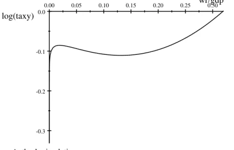
Figure 1. The non-linear relation between remittance and tax ratios in data range of the poor sample (mean 0.029, median 0.014 percent, std.dev. 0.041)
0.00 0.05 0.10 0.15 0.20 0.25 0.30
-0.3 -0.2 -0.1 0.0
wr/gdp
log(taxy)
Source:Author’săsimulation
For the poorer sample, equation (1b) shows a negative impact of remittances from 1.9 percent to 13 percent and a positive one outside this interval (see Figure 1). However, there are many observations below 1.9 percent but not many above 13 percent. Indeed, the panel average in the simulations below is at about 1.7 percent for the poorer countries. The regression works much better when I use the natural log of the tax variable for poorer countries and the version without logs works better for the richer sample.18 The different specifications and the strong non-linearities with many countries on the different sides of the extrema suggest that further dis-aggregation and analyses of heterogeneity could yield further insights. For the richer panels, remittances have a negative direct impact on the tax ratio in equation (1a). The savings ratio has a u-shaped impact with a minimum at 19.7 percent in the richer sample and an inverted u-shape with a maximum at 20.6 percent in the poorer sample. Therefore, we look at the impact of remittances on savings next.
sit = c0,i + 0.55s it-1 + 71.7log(1+wit) -105log2(1+ wit) + 9.0git-1 + 27.7log(1+dit) -
0.57pit-1 (2a)
(0.00) (0.0003) (0.064) (0.013) (0.04) (0.005)
Periods: 26 (1976-2005); countries: 46; Obs.: 457; S.E.:3.29; J-stat: 172.8; p(J) = 0.045.
sit= f0,i+0.668sit-1+ 51.8wit-1-216.7wit-1 2-0.0072pit2-25.4dit + 52.8dit-12 +
18.7(NM/L) it (2b)
(0.00) (0.0034) (0.03) (0.0003) (0.038) (0.0073) (0.0025) Periods: 6 (1980-2005); countries: 32; Obs.: 65; S.E.: 3.3; J-stat.: 26.83; p(J): 0.14
In both samples, worker remittances enhance the savings ratio, because the inverted u-shape effect has a negative slope only when remittances are more than 40.6 percent of the GDP for the richer sample in equation (2a) and 12 percent for the poorer sample; both values are higher than average plus two standard deviations.
There are some other interesting effects in these regressions. The effect of development aid on savings has been debated for decennia (see Doucouliagos and Paldam (2006) for a survey). One possibility for this is coming out of our regressions. In richer countries, aid enhances savings, but in poorer countries, aid reduces savings until it is 24 percent of the GDP, when ignoring the lag. This is plausible in the sense that in poorer countries more money goes to emergency and poverty fighting – to present needs rather than to future needs -, and this money may be matched by that of the government and thereby contribute to a reduction in savings. For richer countries, especially when aid is tied to trade, such as buying machines from the donor country, imperfect fungibility of money allows driving aid into savings and investment rather than consumption. In short, the controversies of the past may be due to panel heterogeneity, stemming from different behaviour of poor and less poor countries. Moreover, in both samples, higher public expenditure on education reduces the savings ratio, which probably is the case because these countries have imperfect credit markets concerning investment in human capital, forcing people to save before investing in education. Then, higher public expenditure on education reduces the pressure to save before schooling. Finally, it seems remarkable that net immigration enhances savings in the poor sample. Probably this is the case because migrants bring some savings with them at amounts higher than the average value in the country, which is not the case in the richer sample19. From the perspective of this
paper, these variables mainly serve the purpose of avoiding an omitted variable bias.
Next, we look at public expenditure on education in order to see how they depend on tax ratios, savings ratios, remittances and aid.
Pit =
h0,I +0.8Pit-1 -0.03Pit-12 +0.77log(TAXYit) +17.9wit–76.2wit2 -19.78dit +91d2it
+0.21pit-5 (3a)
(0.0013) (0.17) (0.003) (0.001) (0.0001) (0.006) (0.0015) (0.0002)
Periods: 20 (1981-2005); countries: 29; Obs.: 169; S.E. = 0.45; J-stat.:8; p(J) = 0.53.
P = k0,i +0.86P it-1 -0.028Pit-1 2 +0.049TAXY it + 1.98dit-5 +0.14LOGwit-1
-21.66w2it -5.4d2it (3b)
(0.00) (0.014) (0.0013) (0.003) (0.0013) (0.015) (0.1003)
Periods: 24 (1982-2005); countries: 29; obs.:182. S.E.: 0.33; J-stat.: 63.4; p(J).: 0.036.
For both groups of countries we find also a quadratic term of the lagged dependent variable. Higher tax revenues are used for higher public expenditure on education. Remittances, often used for private financing for education, induce governments first to increase and then to decrease public expenditure on educationăwithăaămaximumăofă11.7ăpercentăinăricherăcountries’,ăequationă(3a),ă and 5.4 percent in poorer countries. Development aid has a u-shaped effect in the richer sample with a minimum at 10.8 percent and an inverted u-shaped effect in the poorer sample effect with a maximum near 18.3 percent. Richer countries tend to reduce public expenditure on education when getting more aid and poorer countries tend toincrease it before the extremum. Savings have no direct impact on public expenditure on education.
groups are on average. There will also be a strong sensitivity concerning the size of the shock, which may lead into areas with changed slopes.
5. Effects of increasing remittances: baseline simulation and shocks compared
We simulate the above equations with respect to the endogenous variables in order to analyze the effect of changes in remittances on savings ratios, tax ratios and public expenditure on education as a share of GDP. The other variables might also be affected by remittances and the differentiated variables, but we treat them as autoregressive processes, cutting off feedback effects and isolating the effects under consideration.20 For the richer sample, the autoregressive assumption refers to remittances per unit of GDP, the growth rate of the GDP per capita, and the development aid per unit of GDP. For the poorer countries, they regard remittances/GDP, aid/GDP and net immigration per unit of the labour force. In all cases, initial values are constructed by regressing the dependent variable on a constant and a linear or quadratic time trend for some periods with some overlap with the period of estimation.
5.1. Baseline simulations and shocks in the richer sample
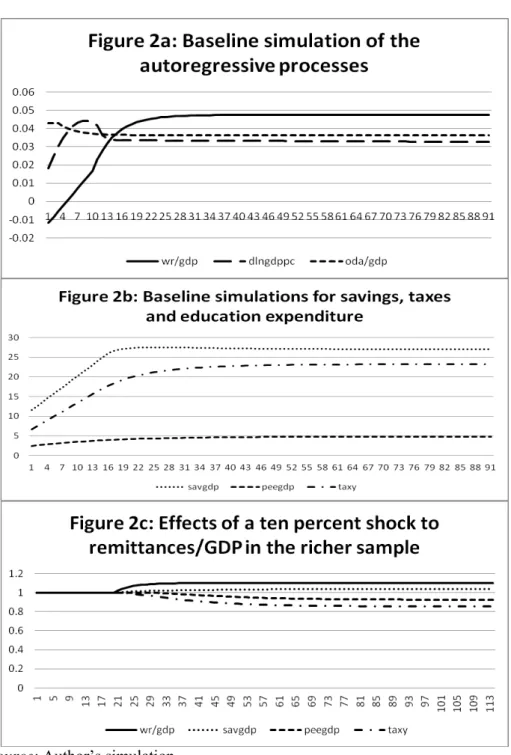
Figure 2a shows the autoregressive processes. The GDP per capita has increasing growth rates until 1970 and then they fall to a little more than three percent. Worker remittances go to about 4.7 percent of GDP and aid to about 3.6 percent. For the richer sample, remittances are larger than aid.
Figure 2b shows the simulation of the dependent variables of equations (1a-3a). Savings go up to 27 percent of GDP, taxation at about 23 percent and public expenditure on education remains below 5 percent.
The consequences of a ten percent shock to remittances/GDP ratio are shown in Figure 2c. The increase in the savings ratio runs up to almost 4 percent of the baseline value. Government variables fall though: the tax ratio by 15 percent below baseline and public expenditure on education up to 7.5 percent. The government withdraws in the richer sample when remittances increase and government variables fall at the same order of magnitude as remittances increase. Smaller shocks lead to qualitatively similar results. If we increase the shock to 60 percent, the system collapses as public expenditure on education go extremely negative and savings and tax ratios extremely positive. This might indicate that parameter values have to change when the shock is large as suggested by the Lucas critique. On the other hand, permanent shocks of 60 percent are very unlikely to occur and therefore elasticity changes may remain low too.
Figure 2. Baseline simulation and ten percent shock for the richer sample
5.2. Baseline simulations and shocks in the poorer sample
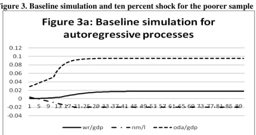
Figure 3a shows the autoregressive processes. Aid is going to 9.5 percent of GDP and therefore is much larger than remittances. Remittances remain below 1.8 percent. Therefore, they are to the left of the local maximum in Figure 1, where the slope is positive up to a value of 1.9 percent.21 Net immigration falls to a negative 2 percent.
Figure 3b shows that savings remain below 15 percent of GDP, but taxes go beyond 25, and public expenditure on education go to 6.5 percent.
Figure 3c shows that a ten percent shock of remittances increases the savings ratio as well as, unlike the previous sample, the public expenditure on education and the tax ratio. Again, smaller shocks lead to qualitatively similar results. If the shock goes to 39.6 percent or higher, the tax ratio reacts slightly negatively because the shock leads far into the area of a negative relation of remittances and taxes in equation (1b) and Figure 1, the range of 1.9 to 13 percent discussed above. The Lucas critique was written in the times of log-linear macroeconomic models with constant elasticities. It is very plausible that the Lucas critique indeed holds here because of the high non-linearity of Figure 1, which does not support a constant-elasticity assumption even for constant parameter estimates.
Figure 3. Baseline simulation and ten percent shock for the poorer sample
Source:Author’săsimulation
6. Summary and conclusion
Summing up, savings increase through remittances in both samples. In the richer sample, remittances reduce taxes and higher savings reinforce this. In the poorer sample, a highly non-linear effect of remittances on taxation is present, which leads to higher savings and taxes for small and medium size shocks, but to negative effects on tax ratios for very high shocks. Public expenditure on education is negatively affected in the richer sample, although higher remittances have a positive effect but lower tax ratios have a negative effect. In the poorer sample too, public expenditures on education increase directly through remittances, but there is no fall in tax ratios for shocks below 39.6 percent of the remittance ratio and therefore the total effect is also positive for the public education money.
clearly benefits from remittances as far as savings, tax ratios and public expenditure for education are concerned because the government acts complementarily, which may contribute to growth. These effects can be viewed as a return to earlier emigration and a (partial) compensation for the implied brain drain. These returns though should not lead to a reduction of efforts achieving higher growth. Especially an entrance of the richer sample into the high-technology areas will be difficult with hesitant education policies. But policy conclusions also depend on interactions with others issues appearing in government budgets.
References
Abdih, Y., Barajas, A., Chami, R. Ebeke, C. (2012), Remittances Channel and Fiscal Impact in the Middle East, North Africa, and Central Asia, IMF WP
12/104, April.
Adams, R.H. Jr., Page, J. (2005), Do International Migration and Remittances Reduce Poverty in Developing Countries?, World Development, Vol. 33, No.10, pp. 1645-1669.
Arellano, M., Bover, O. (1995), Another look at the instrumental variable estimation of error-components models, Journal of Econometrics Vol. 68, pp. 29-51.
Asteriou, D., Hall, S.G. (2011), Applied Econometrics, 4th edition, Palgrave Macmillan, New York.
Baltagi, B.H. (2008), Econometric Analysis of Panel Data, 4th edition, John Wiley, Chichester.
Bazzi, S., Clemens, M.A. (2010), Blunt Instruments: A Cautionary Note on Establishing the Causes of Economic Growth, CGDEV WP, 171, July.
Blundell, R., Bond S. (1998), Initial conditions and moment restrictions in dynamic panel data models, Journal of Econometrics, 87: 115–43.
Bun, M. J. G., Windmeijer, F. (2010), The Weak Instrument Problem of the System GMM Estimator in Dynamic Panel Data Models, Econometrics Journal, 13 (1): 95-126.
Davidson, R., MacKinnon, J. (2004), Econometric Theory and Methods, Oxford University Press, Oxford.
Desai, M.A., Kapur, D., McHale, J., Rogers, K. (2009), The fiscal impact of high-skilled emigration: Flows of Indians to the U.S., Journal of Development
Doucouliagos, H., Paldam, M. (2006), Aid Effectiveness on Accumulation: A Meta Study, Kyklos, Vol. 59, No. 2, pp. 227-254.
Ebeke, C.H. (2010), Remittances, Value Added Tax and Tax Revenue in Developing Countries, CERDI Document de travail de la série: Etudes et
Documents, E 2010.30.
Ebeke, C.H. (2012), Do Remittances Lead to a Public Moral hazard in Developing Countries? An Empirical Investigation, Journal of Development
Studies, Vol. 48, No. 8, pp. 1009-1025.
Fosu, A.K., Getachew, Y.Y., Ziesemer, T.H.W. (2012), Optimal Public Investment, Growth, and Consumption: Evidence from African Countries, Department of Economics and Finance, Durham University, Working Paper, No 2012.03.
Freund, C., Spatafora, N. (2005), Remittances: Transaction Costs, Determinants, and Informal flows, World Bank Policy Research Working Paper 3704, September.
Greene, W.H. (2003), Econometric Analysis, 5th Edition. Pearson, New Jersey.
Griffin, K. (1970), Foreign Capital, Domestic Savings and Economic Development, Oxford Bulletin of Economics and Statistics, Vol. 32, No. 2, pp. 99-112.
IMF (2005), World Economic Outlook, Washington, Chap.2, 69-107.
Karpestam, R.P.D. (2012), Dynamic multiplier effects of remittances in developing countries, Journal of Economic Studies, Vol. 39, No. 5, pp.512-536.
Kennedy, P. (2003), A Guide to Econometrics, 5th edition, MIT Press and Wiley, Blackwell.
Lucas, R.E.B. (2005), International Migration to the High-income Countries: Some consequences for Economic Development in the Sending Countries, in Blanpain, R. (ed.), Confronting Globalization, Kluwer, The Hague, Chap. 12.
Masud, N., Yontcheva, B. (2005), Does Foreign Aid Reduce Poverty? Empirical Evidence from Nongovernmental and bilateral Aid, IMF Working paper WP/05/100, May.
Meijers, H. 2012, Does the internet generate economic growth, international trade, or both?, UNU-MERIT Working Paper 2012-050.
Osili, U.O. (2007), Remittances and savings from international migration: Theory and evidence using a matched sample, Journal of Development
Ratha, D. (2004), Understanding the Importance of Remittances, Migration Information Source, Migration Policy Institute, Washington. Download from 28-3-2008.
Roodman,ăD.,ă(2009a),ăHowătoădoăxtabond2:ăanăintroductionătoă“difference” andă“system”ăGMMăinăstata.ăSTATAăJOURNALăVol.ă9,ăIssueă1,ăpp.ă86ă– 136. Roodman, D. (2009b), A Short Note on the Theme of Too Many Instruments,
Oxford Bulletin of Economics and Statistics 71, 135–158.
Schneider, F., Enste, D. (2000), Shadow Economies: Size, Causes, and Consequences, Journal of Economic Literature, March, Vol. 38, No. 1, pp. 77-114.
Smith, R.P., Fuentes, A.-M. (2010), Panel Time-Series, cemmap course, April 2010. Download 24 Aug 2011.
Soto,ăM.ă(2009)ăSystemăGMMăestimationăwithăsmallăsample,ăInstitutăd’Anàlisiă Econòmica,ăBarcelona,ăJuly.
Wei, Y., Balasubramanyam, V.N. (2006), Diaspora and Development, The
World Economy, Vol. 29, No.11, 1599-1609.
Ziesemer, T. H. W. (2008), Worker remittances and government behaviour in the receiving countries, UNU-MERIT WP 2008-029.
Ziesemer, T.H.W. (2010a), The impact of the credit crisis on poor developing countries: Growth, worker remittances, accumulation and migration, Economic
Modelling, Vol.27, No.5, pp. 1230-1245.
Ziesemer, T.H.W. (2010b), Worker remittances in growth regressions: The problem of collinearity, Applied Econometrics and International Development,
Vol. 10, No. 2, 5-12.
Ziesemer, T.H.W. (2011), What Changes Gini Coefficients of Education? On the dynamic interaction between education, its distribution and growth,
UNU-MERIT Working Paper, 2011-053.
Ziesemer, T.H.W. (2012a), The impact of development aid on education and health: Survey and new evidence from dynamic models, UNU-MERIT Working
Paper, 2012-057.
Appendix A: List of Countries
Countries with GDP per capita above $1200 (2000):
Albania, Algeria, Argentina, Aruba, Belarus, Belize, Bosnia and Herzegovina, Botswana, Brazil, Bulgaria, Cape Verde, China, Colombia, Costa Rica, Croatia, Cyprus, Dominican Republic, Ecuador, Egypt, El Salvador, Estonia, Guatemala, Hungary, Jamaica, Jordan, Kazakhstan, Latvia, Lebanon, Libya, Lithuania, Macao, Malta, Mexico, Morocco, Namibia, New Caledonia, Oman, Panama, Paraguay, Peru, Romania, Russian Federation, Samoa, Seychelles, Slovak Rep., Slovenia, Suriname, Swaziland, Thailand, Togo, Tonga, Trinidad and Tobago, Tunisia, Turkey, Uruguay, Venezuela.
Countries with GDP per capita below $1200 (2000):
Armenia, Azerbaijan, Bangladesh, Benin, Bolivia, Burkina Faso, Cambodia, Cameroon, Comoros, Congo Rep., Cote d'Ivoire, Djibouti, Ethiopia, Ghana, Guinea, Guyana, Haiti, Honduras, India, Indonesia, Kenya, Kyrgyz Republic, Lesotho, Madagascar, Malawi, Mali, Mauritania, Moldova, Mongolia, Mozambique, Nepal, Nicaragua, Niger, Nigeria, Pakistan, Papua New Guinea, Philippines, Rwanda, Senegal, Sierra Leone, Sri Lanka, Sudan, Syria, Tajikistan, Tanzania, Uganda, Ukraine, Vanuatu, Yemen, Zimbabwe.
Appendix B:
Instrumental variables, DWH Endogeneity test, and difference in Sargan tests
This appendix provides the list of instruments used in the regressions, starting with the number of the respective regressions. The first number after a variable gives the first lag used and the second numbers gives the last lag used. These are used as dynamic instruments then (see Baltagi 2008, Chap.8). If only one lag is mentioned, we have a simple standard instrument.
(1a) TAXY,-2,-3;22 SAVGDP,-1,-1; SAVGDP2,-1,-1; (WR(-1)/GDP(-1))2, time dummies; c.
Instrument rank: 158.
(1b) LOG(TAXY),-2,-3; SAVGDP(-1); SAVGDP(-1)2; WR/GDP; (WR(-1)/GDP(-1))2
LOG(WR/GDP); time dummies; c. Instrument rank 94.
(2a) SAVGDP,-2,-4; LOG(1+WR/GDP),-1,-1; LOG2 (1+WR/GDP), -1,-1; D(LOG(GDPPC(-1)));
LOG(1+ODA/GDP),-1,-1; PEEGDP(-1); time dummies; c. Instrument rank: 179.
(2b) SAVGDP,-3,-6;23 WR(-1)/GDP(-1); (WR(-1)/GDP(-1))2; (PEEGDP)2; ODA(-1)/GDP(-1);
ODA(-1)/GDP(-1))2; NM/L; time dummies; c. Instrument rank: 33. (3a) PEEGDP,-2,-3; PEEGDP2,-2,-4; LOG(TAXY); WR/GDP; (WR/GDP)2; ODA(-1)/GDP(-1);
(ODA(-1)/GDP(-1))2; ODA(-2)/GDP(-2); (ODA(-2)/GDP(-2))2; PEEGDP(-5); time dum.; c. Instr.rank: 113.
(3b) PEEGDP,-2,-2; PEEGDP2,-2,-2; TAXY; ODA(-5)/GDP(-5); LOG(WR(-1)/GDP(-1));
(WR/GDP)2; (ODA(-1)/GDP(-1))2 ; time dum.; c. Instrument rank: 76.
DWH endogeneity test of regressors, with one lag as instrument
In the fixed-effects regression corresponding to eq. (1a), the savings variables are endogenous because adding the residuals from the standard24 first stage regressions as an additional regressor in the DWH test yields p-values of
0.0669 for savgdp and 0.02 for savgdp2.
In the fixed-effects regression corresponding to eq. (1b) the worker remittance variable wr/gdp is not endogenous because adding the residuals from the first stage regression as an additional regressor yields a p-value of 0.73 and
p=0.82 for its log version. We assume that the worker remittance variable is not
pre-determined, but exogenous.
In the fixed-effects regression corresponding to eq. (2a), the aid and worker remittance variables are not endogenous because adding the residuals from the first stage regression as an additional regressor yields p-values of 0.81,
0.37 and 0.645 in the order of appearance above. We assume that worker
remittances and aid both are predetermined rather than exogenous, as they may compensate earlier shocks to savings in the richer sample.
In the fixed-effects regression corresponding to eq. (2b) the variables public expenditure on education/GDP, ODA/GDP and net immigration as a share of the labour force aid are not endogenous because adding the residuals from the first stage regression as an additional regressor yields p-values of 0.97,
0.62 and 0.30 in the order of appearance above. As ODA/GDP may indeed
depend on earlier residuals, because in poor countries aid is given because of a lack in the surplus product, it may be pre-determined and we use a lagged instrument. For education expenditure and migration there is hardly any reason
23 The difference-in-Sargan test for the last lag has p = 0.72, indicating a low effect on the J-statistic but the lagged dependent goes into the expected direction.
why they should depend on earlier residuals of savings and we assume that they are exogenous.
In the fixed-effects regression corresponding to eq. (3a), all the contemporaneous regressors are not endogenous because adding the residuals from the first stage regression as an additional regressor yields p-values of 0.67
for taxy, 0.46 for wr/gdp, 0.66 for (wr/gdp)2, 0.33 for oda/gdp and for its square
0.16. As ODA/GDP may indeed depend on earlier residuals, because in many
countries aid is given because of lacking education money,25 it may be pre-determined and we use a lagged instrument. For taxes and remittances, we assume that they are exogenous.
In the fixed-effects regression corresponding to eq. (3b) all the contemporaneous regressors are not endogenous because adding the residuals from the first stage regression as an additional regressor yields p-values of 0.71
for taxy, 0.54 for (wr/gdp)2, 0.38 for oda/gdp squared. As ODA/GDP may
indeed depend on earlier residuals, because in poor countries aid is given because of the lack in education money, it may be pre-determined and we use a lagged instrument. For taxes and remittances there is hardly any reason why they should depend on earlier residuals of peegdp and we assume that they are exogenous.
Unfortunately, there seems to be no test for the question whether a regressor is exogenous or predetermined. Making the assumptions differently from what we did above leads in all cases to lower values of the coefficient of the lagged dependent variables, although they should probably be even higher to correct the bias of 1/T, and often we get in addition other worse results. We do not hesitate to admit that the assumptions have been made in a way to get the results as consistent as possible with econometric theory, here the upward correction of the fixed effects bias in the coefficient of the lagged dependent variable.