Network
Adam Ponzi*, Jeffery R. Wickens
Neurobiology Research Unit, Okinawa Institute of Science and Technology (OIST), Okinawa, Japan
Abstract
Slowly varying activity in the striatum, the main Basal Ganglia input structure, is important for the learning and execution of movement sequences. Striatal medium spiny neurons (MSNs) form cell assemblies whose population firing rates vary coherently on slow behaviourally relevant timescales. It has been shown that such activity emerges in a model of a local MSN network but only at realistic connectivities of 10*20% and only when MSN generated inhibitory post-synaptic potentials (IPSPs) are realistically sized. Here we suggest a reason for this. We investigate how MSN network generated population activity interacts with temporally varying cortical driving activity, as would occur in a behavioural task. We find that at unrealistically high connectivity a stable winners-take-all type regime is found where network activity separates into fixed stimulus dependent regularly firing and quiescent components. In this regime only a small number of population firing rate components interact with cortical stimulus variations. Around 15% connectivity a transition to a more dynamically active regime occurs where all cells constantly switch between activity and quiescence. In this low connectivity regime, MSN population components wander randomly and here too are independent of variations in cortical driving. Only in the transition regime do weak changes in cortical driving interact with many population components so that sequential cell assemblies are reproducibly activated for many hundreds of milliseconds after stimulus onset and peri-stimulus time histograms display strong stimulus and temporal specificity. We show that, remarkably, this activity is maximized at striatally realistic connectivities and IPSP sizes. Thus, we suggest the local MSN network has optimal characteristics – it is neither too stable to respond in a dynamically complex temporally extended way to cortical variations, nor is it too unstable to respond in a consistent repeatable way. Rather, it is optimized to generate stimulus dependent activity patterns for long periods after variations in cortical excitation.
Citation:Ponzi A, Wickens JR (2013) Optimal Balance of the Striatal Medium Spiny Neuron Network. PLoS Comput Biol 9(4): e1002954. doi:10.1371/ journal.pcbi.1002954
Editor:Lyle J. Graham, Universite´ Paris Descartes, Centre National de la Recherche Scientifique, France ReceivedSeptember 10, 2012;AcceptedJanuary 13, 2013;PublishedApril 11, 2013
Copyright:ß2013 Ponzi and Wickens. This is an open-access article distributed under the terms of the Creative Commons Attribution License, which permits unrestricted use, distribution, and reproduction in any medium, provided the original author and source are credited.
Funding:This work is entirely funded by Okinawa Institute of Science and Technology. The funders had no role in study design, data collection and analysis, decision to publish, or preparation of the manuscript.
Competing Interests:The authors have declared that no competing interests exist. * E-mail: [email protected]
Introduction
The striatum forms the main input to the Basal Ganglia (BG), a subcortical structure involved in reinforcement learning and action selection. It is90%composed of medium spiny neurons (MSNs) which inhibit each other through a local network of collaterals, receive excitatory projections from the cerebral cortex and are the only cells which project outside the striatum. Because of its inhibitory structure the MSN network is often thought to act selectively, transmitting the most active cortical inputs downstream in the BG while suppressing others. However studies show that local MSN network connections are too sparse and weak to perform global selection and their function remains puzzling.
Many studies of neural response to sensory stimuli and behavioural task events throughout the brain have found that cells display large highly repeatable variations in firing rate on slow behaviourally relevant time scales. In the striatum tonic and phasic MSN activity patterns have been observed locked to task [1–3] and reward predicting events [4–7]. Several studies show that individual MSNs display diverse response profiles with phasic activity peaks not simply at stimulus onset and offset but broadly distributed across the whole spectrum of delays after task events [8–10].
Since MSN network connectivity is sparse and weak it has been assumed in-vivo MSN firing patterns simply reflect cortical driving. Indeed if the roughly 10000 cortical inputs an MSN receives covary, even weakly [11,12], on slow timescales cumu-latively they could generate large modulations in MSN activity on similar time scales. It is important to understand how temporally varying cortical inputs are transformed by the MSN network and possibly interface with intrinsically MSN network generated population and cell assembly dynamics.
Several other recent studies have suggested the possibility that rather than acting independently MSNs may act coherently in cell assemblies [14,15]. Cell assembly activity is commonly observed throughout the brain [14–22]. However in contrast to cortical studies where cell assemblies are often defined through precise repetitive spiking relationships striatal studies suggest that MSNs do not synchronize on precise timescales but rather display coherently varying firing rates generated by coherent burst firing episodes on slower timescales [14,15,23]. In-vitro investigations [14,24,25] found that MSN cell assemblies fire coherently in recurrent sequential episodes and generate complex spatio-temporal patterns while network transition matrices display abrupt transitions between different active cell assemblies.
In recent modeling work [26] we showed that the local MSN network even when driven by constant cortical excitation can generate such slowly varying cell assembly dynamics providing cells are excited just above firing threshold. In this ‘balanced’ situation even small changes in network generated inhibition or cortical excitation can cause cells to switch between firing and quiescent states. Network generated activity was in close agree-ment with experiagree-ment only at striatally relevant connectivity of around10*20%.
Here we investigate how sudden switches in cortical driving, as might occur in sensory driven behavioural tasks interacts with MSN network generated chaotic cell assembly activity. We show that stimulus specific cell assemblies can be reliably activated in sequence locked to stimulus switch times, resulting in slowly varying peri-stimulus time histograms (PSTH). Thus rather than generating a static stimulus dependent activity pattern we suggest the local MSN network is optimized to generate stimulus dependent dynamical activity patterns for long time periods after variations in cortical excitation. We investigate how this activity depends on network parameters and find that MSN task modulation is optimized in a marginally stable transition regime which occurs at striatally relevant connectivities and synaptic strengths. We discuss how these properties may be utilized in
temporally delayed reinforcement learning tasks strongly recruit-ing the striatum.
Results
Networks display stimulus switching induced reproducible patterns
In this section we illustrate stimulus onset locked cell assembly dynamics using an example time series. We show that the MSN network can generate prolonged sequences in response to sudden changes in otherwise constant cortical stimuli. Thus we show that the MSN network produces a dynamic sequence rather than a static state of active and quiescent cells due to the MSN network dynamics rather than the cortical drive.
In Figure 1(a) we show a spike raster plot from a500cell MSN network simulation of connectivity r~0:22. The simulation is subject to an input switching protocol where two different stimuli, each characterised by a fixed set of cortical input rates (see Methods), are applied for two seconds each in alternation repeatedly. Cells have been ordered by a clustering algorithm (see Methods) applied to only one of the stimuli, B, and each of the 30 clusters is coloured differently. As can be seen individual cells fire spikes in episodic bursts lasting up to many hundreds of msecs. The MSNs fire approximately periodically with period two seconds, the period of the forcing stimulus. Most cells do not fire throughout the whole duration of a stimulus but ‘phasically’ at specific epochs often several hundred msecs after onset of a particular stimulus and lasting for only a short time.
In order to quantify the reproducibility of the dynamics we calculate the two-time firing rate similarity [14,21,22,27,28]. Similarity is just the scalar product of the vectors of cell firing rates at two different times,t1and t2. Similarity can take values ranging from 0, meaning firing rate vectors are orthogonal, to 1, meaning firing rate vectors are identical. Figure 1(b) shows a 8|8second mean similarity matrix, M(t1,t2) constructed by moving an eight second segment through the time series in steps of four seconds to create an average similarity with periodicity of the stimulation period (see Methods).
We denote by B(a,b) the ‘block’ of time points such that
avt1vaz2andbvt2vbz2. Therefore the blocksB(0,0), and
B(2,2)describe the mean similarity within a given presentation of respectively stimulus A or B. Sometimes this seems ‘diagonal’ (e.g. stimulus B,B(2,2)) and sometimes more ‘block-like’ (e.g. stimulus A, B(0,0)). In stimulus B the similarity drops off rapidly as t1
increases away from the diagonal t1~t2 (for any 2vt2v4)
showing that the firing activity moves through a rapid succession of different states during stimulus B (as can also be observed directly in the time series Figure 1(a)). The network therefore not only represents the active stimulus but also the time elapsed since stimulus onset. On the other hand activity during stimulus A is more ‘fixed point’ like, where time elapsed from onset is not strongly encoded.
The blocks B(2,0) and B(4,2) describe similarity in firing activity between a given stimulus, respectively A and B, and the immediately following stimulus, respectively B and A. As can be seen similarity is weak in these blocks demonstrating that the network activity is able to discriminate the stimuli.
The blocks B(4,0) and B(6,2) describe similarity between a given stimulus, respectively A and B and thenextpresentation of the same stimulus. In particular in stimulus B activity drops off rapidly ast1increases away from the diagonalt1~t2z4(for any 2vt2v4) demonstrating that the network activity not only moves
through a sequence of different states, but that these state Author Summary
sequences are reproducibleacross different presentations of a given stimulus.
These results demonstrate that an inhibitory spiking MSN network model can generate sequential patterns of activity for several hundred msecs after stimulus onset which are reproducible across different presentations of the same stimulus, but different for different stimuli. This is true even though the excitatory input strengths are fixed for the duration of a stimulus (except for random fluctuations). Thus the activation of cells is not simply determined by the input strengths. If this were the case (roughly speaking) the most strongly excited cells in any particular stimulus would remain active throughout that stimulus period while the least strongly activated would remain quiescent throughout the stimulus. Since the mean excitatory input strength is the same in both stimuli the onset locked patterns result only from the redistribution of excitation across MSNs; an increase in mean excitation level is not required. This is because cells are balanced close to firing threshold where even small variations in input drive cause a large change in the distribution and temporal evolution of activity across the inhibitory asymmetrically connected network. Thus balanced network activity provides cells with a large diversity of strong temporal responses to a given stimulus, rather than generating a static state of active and quiescent cells. Moreover clusters formed from many cells can also display this behaviour as observed in the time series Fig. 1(a).
Recognition of stimuli through sequential activations remains stochastic however; on some trials a stimulus fails to generate its normal patterns. These failures may correspond to error trials in a behavioural task. Stochastic stimulus recognition is not due to the random fluctuations in excitation, but an effect of the chaotic network dynamics, also occurring in deterministic spiking network simulations as described in Supplemental Text S1. These results extend those briefly reported in our previous publication [29]. In the following we investigate why this activity occurs and under what MSN network conditions it occurs maximally.
Stimulus onset locked reproducible dynamics optimized near striatal connectivity
We have demonstrated that stimulus onset locked reproducible dynamics can occur in network simulations, but how does it depend on the network parameters such as connectivity and
connection strength? To investigate these issues quantitatively we calculate mean similarity profiles for simulations of 500 cell networks. In previous work [26] (and see Model) we have suggested that a 500 cell network can provide a reasonable representation of real MSN network activity. This is because it respects both the striatally relevant MSN connection probability, of about 15%, and the approximate number of cells, *500, contacted by a given MSN since only a proportion of the MSN cells *15% are depolarized to firing threshold by cortical excitation. We demonstrate here that the reproducibility of stimulus onset locked dynamics is maximized at striatally relevant connectivities.
Figure 2(a) shows cross-sections from mean similarity matrices
MT(t) (see Methods and Figure 2(b)) calculated from a 500 cell connectivity r~0:18 network simulation of 180 seconds, after discarding a 12 second transient. As in the example time series above (Figure 1(a)) here network simulations have two stimuli, each presented for two seconds, alternately. Each profile shows the similarity between a 100 msec window centered on a given epoch
T msecs after the onset of a stimulus and another 100 msec window at a later timeTzt, averaged across all presentations of both stimuli. The time lagst extend for 5 seconds, that is to a point near the end of the next presentation of the current stimulus. In other words these are profiles along a horizontal (or vertical) slice from the pointt1~t2~T through a mean similarity matrix like the one shown in Figure 1(b) as schematically illustrated in Figure 2(b).
The late epoch T~800msec similarity profile, Figure 2(a, cyan), describes how similarity behaves far from stimulus onset. After about half a second (t&500msec) firing activity patterns decorrelate and similarity decays to its background level of about 0:93. This is the level of similarity between firing activity patterns separated by long time periods under a constant stimulus. At time lagt~2000{T~1200, the switch to a different stimulus occurs. As can be seen this T~800 similarity profile (cyan) shows a sudden change to a lower level around 0:45. This low level of similarity, in this case close to the similarity level 0:5 of uncorrelated activity, demonstrates that the different stimuli evoke very different activity patterns. At time lagt~4000{T~3200 the onset of the next presentation of the same stimulus occurs and similarity returns to its background level of around0:93. Similarity
Figure 1. Stimulus onset locked reproducible cell assembly sequences.Cell raster plot time series segment for the 500cell network simulation with connectivityr~0:22, inhibitory neurotransmitter timescale timescaletg~50msec and synaptic strength parameterk~1so that peak synaptic conductance is3:4=(50|0:22)~0:34 nSand peak IPSP size&230mV, corresponding to Figure 8(e,f).2|2second input switching stimuliAandBare indicated on bottom axis. Cells are grouped and coloured by k-means clusters with 30 clusters applied to only stimulusB. All cells active in stimulusBshown. Elipses indicate cell cluster bursts which appear to repeat across multiple presentations of stimulusB. (b) 8 second similarity matrixM(t1,t2)averaged across the whole 180–12 second time series, including 42 presentations of each stimulus, a segment of which is shown in (a). Colours shown in key. Stimulus A is presented during periods0*2and4*6and stimulus B is presented during periods2*4and
6*8secs.
shows a (broad and weak) peak centered exactly on time lag t~4000msec. Thus activity is most similar at the same epochT
in the next presentation of the current stimulus, even at this late epoch T~800msec after stimulus onset. The existence of this peak demonstrates that the dynamical evolution after stimulus onset is reproducible across presentations.
The behaviour is different at epochsT close to stimulus onset, such asT~100msec (black). Activity in this early epoch is much less similar to the stimulus’ background activity, as shown by the decay to a much lower level of similarity (around 0:8) than the
T~800epoch (cyan) case. At time lagt~2000{T~1900, the switch to a different stimulus occurs. Similarity drops to a lower level, but not as low as the epochT~800(cyan) level. Thus firing activity early after a stimulus switch is more similar to the previous (and subsequent) stimulus than later after the switch (see Discussion). Again similarity shows a peak att~4000, the exact same epochT in the next presentation of the current stimulus. This T~100 epoch similarity peak is much sharper than the
T~800(cyan) one. Similarity profiles MT(t) at intermediate T
show decreasing t~4000 peak sharpness with increasing T
indicating that the reproducibility of the dynamical evolution does not continue indefinitely.
We now investigate how reproducibility of dynamical evolution depends on network connectivity. As explained in the Model section when we vary connectivityrwe rescale the connection strength by the connection probability so that the mean level of inhibition on a cell is unchanged by the connectivity variation.
The reproducibility at epoch T of the stimulus onset locked dynamics can be quantified by the difference in the height of the t~4000 peak seen in Figure 2(a) and the background level as a function of epochT. Indeed if the stimulus onset locked dynamical evolution were not reproducible at a given epochTthen the epochT
similarity profile would not show at~4000peak and similarity would remain at the peak level of&0:93, like theT~800(cyan) similarity profile does. Thus we calculate the average meanbackgroundsimilarity,
MB(T)~SMT(t)T
950vtv1050 and peak similarity MP(T)~ SMT(t)T3950vtv4050 obtained by averagingMT(t) over the time
lagtranges950vtv1050and3950vtv4050, respectively, (shown
by the vertical lines in Figure 2(a) and illustrated schematically in Figure 2(b)) for different epochsT after stimulus onset.
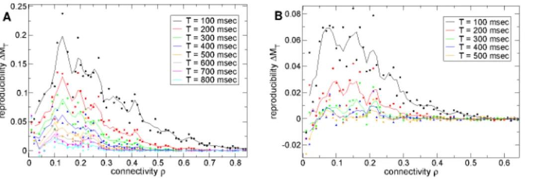
The quantity DM(T)~MP(T){MB(T), is plotted versus
connectivity for several epochs T in Figure 3(a). At high connectivity rw0:5, DM(T) approaches zero for all epochs T. Below this connectivity it starts to increase, displaying a peak around connectivityr~0:1*0:2before decreasing again. Around connectivityr&0:15,DM(T)is significantly greater than zero up to about epochT~800msec (cyan line) indicating reproducible stimulus locked dynamics persists for this long after stimulus onset at this connectivity. Most interestingly reproducible stimulus locked activity appears optimal at connectivities close to real striatal connectivity.
Peak in dynamical reproducibility is robust to decrease in time scale of inhibition
In the Model section we explain that the time scale of inhibitory neurotransmitter decay is set by the parametertg. In the above
this has been set totg~50msecs in accordance with Janssen et al.
[30] which shows a time course of MSN IPSP with a half life of recovery of about 30–40 msec. However a fairly large range of values has been found in various studies depending on experi-mental conditions [31–35]. Here we investigate network behaviour
when tg is reduced to 20 so that the decay half-life
ln(2)tg~14msec.
Figure 3(b) shows the same computation of the reproducibility of stimulus onset locked dynamicsDM(T) shown in Figure 3(a) except using the reduced setting fortg. EvidentlyDM(T)shows a
very similar behaviour at this lowertg, including the peak around
connectivity r~0:1*0:2. The magnitude of the effect is much reduced however as can be seen by the peak height. Furthermore even at optimal connectivity,DM(T)is only significantly different
from zero up to about epochT~300msec. However the results presented above, in particular the peak in DM(T) at striatally
relevant connectivity are robust to at least60%reduction intg.
Peaks in dynamical reproducibility and distinguishablity occur when inhibitory connections have near striatal strength
We can also ask how the reproducibility of stimulus onset locked dynamics, DM(T), depends on the strength of inhibitory Figure 2. Mean firing rate similarity shows peak at same time epoch in the following presentation of current stimulus.(a) Mean similarity profilesMT(t)for connectivityr~0:18network simulation versus time lagt. Firing rate similarities calculated using 100 msec window incremented in 10 msec steps. EpochsT after stimulus onset shown in key. Bars indicate sem. Vertical lines indicate averaging periods (see Figure 2(b)). 500 cell network simulation of length 180–12 seconds under a2|2second input switching protocol. Inhibitory neurotransmitter timescaletg~50msec. Synaptic strengthk~1so that peak synaptic conductance is3:4=(50|0:18)~0:38 nSand peak IPSP size &280mV(b)
Illustration of mean similarity profilesMT(t)and calculation of averagesMB(T),MD(T),MP(T). For example the green solid line showsM300(t) whileMB(300) is the mean similarity in the intersection of the green solid line and the two diagonal lines denoted byMB(T)at time lags t~950,1050.
connections. In the Model section we explain that the connection strength parameter kM was chosen to be 3:4 nS in order to
generate realistic IPSPs of around 250mV[26] at connectivities around r~0:2 when the postsynaptic cell is close to firing threshold and the inhibitory neurotransmitter timescale has the valuetg~50msec. At these parameter values the peak
conduc-tance generated by a spike is3:4=(0:2|50)~0:34 nS(see Model section.) Here we fix the connectivityr~0:2and timescaletg~50
and vary the synaptic strength around the value which produces IPSPs of realistic size. Thus the peak conductance is set to be k0:34 nSandkvaried so thatk&1recovers IPSPs of realistic size. In Figure 4 we show that variation withkalso produces a peak in
DM(T)for epochs up to aboutT~600msec after stimulus onset. The peak is very close tok~1. Remarkably the maximum occurs close to the value of connection strength which recovers IPSPs close to experimentally observed size.
In Figure 4(b) we also show a stimulusdistinguishabilitymeasure
DM2(T)~MB(T){MD(T). Here thedifferentstimulus similarity, MD(T)~SMT(t)T
2950vtv3050 is obtained by averaging MT(t)
over the time lagtrange,2950vtv3050(shown by the vertical
lines in Figure 2(a) and illustrated in Figure 2(b)). The distinguish-ability of background activities under the two stimuli is given by the large epochT results, for example byDM2(800). A value of
zero indicates that similarity between firing activity at two well separated time points in a given stimulus is the same as between two different stimuli, and thus activity is solely dependent on the network irrespective of the stimulus. Stimulus distinguishability
DM2(800) (cyan) also remarkably has a peak near k~1 in the striatally relevant region. For shorter epochs after stimulus onset, for example T~100 (black), the quantity DM2(100) is smaller because soon after stimulus onset firing activity resembles the previous stimulus. Stimuli become more distinguishable as time elapses (see Discussion.)
MSN network shows dynamical regime transition as connectivity and connection strength are varied
We have shown that the reproducibility of stimulus onset locked dynamical evolution and stimulus distinguishability are optimized in the striatally relevant parameter region of connec-tivity and connection strength. We now investigate why this should be. Here we show that the peaks occur near a transition in network activity which occurs in the striatally relevant parameter region and demonstrate the nature of the transition. In this section we investigate 500 cell network simulations underconstant
(randomly fluctuating) excitatory drive without the stimulus switching.
Figure 3. Stimulus onset locked reproducible dynamics maximal at striatal connectivity. (a) Strength of stimulus onset locked reproducible dynamicsDM(T)(see text) versus connectivityrfor several different epochsT after stimulus onset (see key) corresponding to Figure 2(b). Inhibitory neurotransmitter timescale tg~50msec. Synaptic strength parameterk~1so that peak synaptic conductance varies as 3:4=(50r)nSand peak IPSP size as&(50=r)mV. (b) Same as (a) except inhibitory neurotransmitter timescale reduced by60%totg~20msec. Synaptic strength parameterk~1so that peak synaptic conductance varies as3:4=(20r)nSand peak IPSP size as&(80=r)mV. (a,b) 500 cell network
simulations of length 180–12 seconds under the2|2second input switching protocol. Points show actual values, solid lines show three point average.
doi:10.1371/journal.pcbi.1002954.g003
Figure 4. Stimulus onset locked reproducible dynamics and stimulus distinguishability maximal at striatal connection strengths.(a) Strength of stimulus onset locked reproducible dynamics DM(T)(see text) versus synaptic strength parameter kfor connectivityr~0:2and timescale of inhibitory neurotransmittertg~50msec. Actual peak conductance is given byk0:34 nSandk~1generates realistic peak IPSP sizes of around250mV. Several different epochs T after stimulus onset (see key) for 500 cell network simulations of length 180–12 seconds under a
2|2second input switching protocol. Points show actual values, solid lines show three point average. (b) Same as (a) but stimulus distinguishability DM2(T).
The black points in Figure 5(a) show the minimum inter-spike-interval (ISI) observed for each active cell (cells which fire at least three spikes in the 168 second observation period) in network simulations of different connectivity. At high connectivity the distribution is very broad. Most cells have minimum ISIs of between 10 and 20 msecs but many have much longer minimum ISIs. This indicates that at high connectivity the network displays winner(s)-take-all like activity.
On the other hand at low connectivity the minimum ISI distribution does not show the quiescent component. The transition from a broad distribution to a narrow one appears to occur fairly suddenly around r~0:2 connectivity. This is also observed in the mean minimum ISI (Figure 5(a) red line) which is roughly flat with high value abover&0:5connectivity, but falls off rapidly below around connectivityr~0:2.
The coefficient of variation (CV) of a cell’s ISI distribution, defined as the cell’s ISI standard deviation normalized by its mean ISI, also reveals the connectivity dependent transition. Figure 5(c, green line) shows how this quantity, averaged across all active cells, varies with network connectivity corresponding to Figure 5(a). At connectivities above around r~0:5it is roughly flat with value around0:75indicating that on average cells are firing fairly regularly. Below about connectivityr~0:5it starts to increase and very rapidly below about connectivity r~0:2. Spike time series’ become signifi-cantly more bursty than Poissonian (CVw1) around r~0:15 connectivity. Thus we find a transition from a network state
where the active cells fire mostly regularly to a state where active cells fire in an episodic bursting way.
The proportion of active cells (those that fire at least three spikes in the 168 second observation period) also demonstrates the connectivity dependent transition. This quantity (Figure 5(c), black line) shows a minimum around connectivityr&0:2where about 50%of the network cells are active. On increasing connectivity the
active proportion rises slowly towards about 70% at full
connectivity while on decreasing connectivity it rises rapidly towards 100% activity at zero connectivity. Indeed when fewer cells are active we expect network generated fluctuations to be reduced and the remaining active cells thus fire more regularly, reducing the CV values at higher connectivity.
Thus the network shows a fairly sharp transition from a regularly firing winners-take-all type regime where a proportion of cells are permanently quiescent to a regime where almost all cells are involved in bursty activity. Remarkably actual striatal connectivity of around r~0:17 appears to be in the transition regime.
Figure 5(b,d) show the same quantities but versus the connection strength parameter k for network simulations of connectivityr~0:2. Again network dynamics shows a transition. In the approximate region0:25vkv1, (so that peak IPSP sizes
vary between60mVand250mVand peak synaptic conductances vary between0:085 nSand0:34 nS), the network shows a winners-take-all behaviour. This can be seen from the broad distribution of minimum ISI (Figure 5(b), black points) with some very long
Figure 5. Dynamical regime transition in network activity.(a) Black circles: minimum observed ISI for each active cell in network simulations of different connectivity. Red line: mean of minimum observed ISI across all cells for each network simulation. Synaptic strength parameterk~1so that peak synaptic conductance varies as3:4=(50r)nSand peak IPSP size&(50=r)mV. (b) Same as (a) but versus synaptic strength parameterkfor
connectivityr~0:2. Actual peak synaptic conductance is given byk0:34 nSandk~1generates realistic peak IPSP sizes of around250mV. (c) Green line: mean ISI coefficient of variation (CV) across all cells in network simulations of different connectivity corresponding to (a) (bars indicated sem). Black line: proportion of active cells (those that fire at least three spikes in the 168 second time series). Red line: mean relative entropy,SRETof 100 msec firing rate distribution across all cells rescaled by8=log(N)whereNis the number of active cells (see text) (bars indicated sem). (d) Same as (c) but corresponding to (b). (a,b,c,d)N~500cell network simulations under constant (randomly fluctuating) excitation without stimulus switching. 180–12 second time series. Inhibitory neurotransmitter timescaletg~50msec.
minimum ISI, the very high mean ISI (Figure 5(b), red line), the proportion of active of cells (Figure 5(d), black line) indicating that less than 75% of the network is active, and the low mean ISI CVv1(Figure 5(d), green line), indicating that network
simula-tions include many relatively regularly firing cells. At higherkw1,
(peak IPSP size w250mV and peak synaptic conductance
w0:34 nS) on the other hand, the network appears to be in a
highly active state with many burst firing cells. This is indicated by the high ISICVw1, the narrow distribution of minimum ISI with
low mean ISI and the fact that most of the network cells are active. At very lowkv0:25(peak IPSP sizev60mVand peak synaptic
conductancev0:085 nS) however we find another regime where
connection strength vanishes and thus all cells in the network fire perfectly regularly (except for stochastic fluctuations in excitatory input).
Remarkably again the transition between the winners-take-all like regime and the bursty active regime appears to be close to k&1, in the striatally relevant parameter region where presynaptic spikes generate realistically sized IPSP*250mV. Notice also that in both the connectivity r variation and synaptic strength k variation the transition occurs close to a minimum of approxi-mately50%in the quantity of active cells (Figure 5(c,d) black lines). This is also where the mean ISI CV is close to or slightly larger than unity (see Discussion).
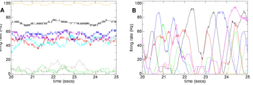
Finally, as an illustration of the different activity in the two regimes, Figure 6 shows rate time series for several cells from a high connectivity (Figure 6(a)) simulation in the winners-take-all regime and a low connectivity (Figure 6(b)) simulation in the active bursty regime. As can be seen, in the winners-take-all regime (Figure 6(a)) firing rates seem to fluctuate mildly around well-defined seemingly stable mean levels. Individual cells appear to have narrow firing rate distributions which overlap only weakly with other cells rate distributions. In contrast in the bursty regime firing rates fluctuate wildly between zero and maxima defined by the cells driving cortical excitations, and appear very unstable, so that cells have broad strongly overlapping rate distributions.
This observation can be quantified by the relative entropyRE (see Methods) between a cell’s firing rate distribution and the
combinedfiring rate distribution of all active cells in a given network simulation. This relative entropy is zero when the firing rate distribution of a single cell coincides with the combined firing rate distribution across all cells. On the other hand it reaches a value log(N)when the firing rate distributions of theN active cells are entirely non-overlapping. The quantity8SRET=log(N)(the factor 8 is included simply for convenient scaling on the figure) is shown
averaged across all cells in the network versus connectivity in Figure 5(c) and versus connection strength in Figure 5(d) by the red lines. As can be seen it also exhibits the transition at striatal relevant parameter settings of r&0:2 and k&1. At lower connectivity or higher connection strength the firing rate distributions of single cells are similar to the distribution across all cells combined. In contrast at higher connectivity or lower connection strength the rate distributions of individual cells are much less overlapping.
Rate dynamics is marginally stable at striatally relevant connectivity and connection strength
Above we have shown that the MSN network displays a transition between a bursty active regime and a winners-take-all like regime as connectivity and connection strength are varied. The transition occurs at striatally relevant parameter settings. Here we demonstrate that the rate dynamics generated by the MSN network model is unstable and chaotic in the bursty active regime but stable in the winners-take-all like regime and thus marginally stable at striatally relevant parameter settings.
The postsynaptically bound inhibitory neurotransmittersgjvary slowly in the MSN network model [26] and essentially act as a low-pass filter of presynaptic spiking activity [26]. By replacing the detailed dependence on presynaptic activity with the presynaptic firing rate we obtain a reduced rate model describing the dynamical activity of the postsynaptically bound inhibitory neurotransmitters gj (see Methods.) The reduced model has exactly the same parameters as the full spiking network model including the inhibitory connectivity structure and excitatory driving. However in order to study the stability of network generated deterministic rate dynamics the noise in the excitatory driving is not included. Again the excitatory driving is fixed for the duration of the simulation without stimulus switching. The conductance based synapses are also replaced by current synapses which do not depend on the postsynaptic membrane potential.
The deterministic rate model shows a very similar qualitative dependence of the number of active cells on connectivity (Figure 7(a) black circles) and connection strength (Figure 7(b) black circles) as the full spiking model (Figure 5(c,d)). A weak minimum is shown at striatally relevant connectivity around r&0:17 and a marked minimum at striatally relevant connection strengthk&1. The same is true for the variation of the relative entropyREwith connectivity and connection strength, (Figure 7(a,b) red diamonds.) As in the full spiking model a fairly sudden transition is seen at striatally relevant connectivity and connection strength.
Figure 6. Firing rate time series show qualitatively different behaviours dependent on connectivity. (a,b) Firing rate time series segments based on 400 msec moving window for several randomly chosen cells from 500 cell network simulations under constant (randomly fluctuating) excitation without stimulus switching. Inhibitory neurotransmitter timescaletg~50msec. (a) Connectivityr~0:75, synaptic strength parameterk~1so that peak synaptic conductance is3:4=(50|0:75)~0:09 nS and peak IPSP size&65mV; (b) Connectivityr~0:07, synaptic strength parameterk~1so that peak synaptic conductance is3:4=(50|0:07)~0:98 nSand peak IPSP size&720mV.
The reduced model is deterministic and since it also lacks the strong instability of the spike generating mechanism we are able to compute the maximal Lyapunov exponent for the rate dynamics of 500 cell networks. This quantity characterises the stability of the rate dynamics. When it is positive the network rate dynamics is chaotic. When it is negative however the network has a found a fixed distribution of firing rates or alternatively some, or all, of the cells firing rates may be varying periodically. As can be seen by the blue crosses in Figure 7(a,b) network rate dynamics is unstable and chaotic in the active bursty regime but stable in the winners-take-all regime. Only in the striatwinners-take-ally relevant parameter regime is the maximal Lyapunov exponent close to zero indicating the network is marginally stable. This point is also known as the ‘edge-of-chaos’ [36–39]. The other quantities, the relative entropy RE and the proportion of active cells show strong fluctuations across simula-tions when the Lyapunov exponent is close to zero. This is due to the simultaneous proximity of stable and unstable states.
Time series examples from simulations of this reduced rate model displaying fixed point, periodic and chaotic activity are shown in Supplemental Text S1. The distribution of fixed point, periodic and chaotic states under variation of connectivityrand connection strengthkis also shown in Supplemental Text S1.
Stimulus onset locked reproducible dynamics mediated by coherently activating cell populations
Above we have demonstrated that temporally extended reproducible sequential dynamics can occur locked to stimulus switches. We have shown this activity occurs maximally near a transition in network activity where rate dynamics is marginally stable and which occurs in the striatally relevant parameter range. However in principle sequential activity could be mediated by a chain of single cells activated in sequence. Coherent activity of cell assemblies [14,15,23–25] has also been observed in the striatum and such population activity could provide a potent force to inhibit and disinhibit downstream targets. Here we investigate whether stimulus onset locked sequential dynamics is also shown by cell assemblies, as well as by individual cells.
The cell spike raster plot time series segment from the intermediate connectivity,r~0:22, 500 cell simulation shown in Figure 1(a) seems to indicate that reproducible stimulus onset locked dynamics is indeed mediated by cell assemblies rather than single cells. Indeed the network appears to switch through different
sequentially activated distributions of active and quiescent cell assemblies (indicated by ellipses) throughout stimulus B, which approximately repeat across different presentations of stimulusB. On the other hand, at high and low connectivity reproducible sequentially activated distributions of active and quiescent cells are not observed (see time series described in Supplemental Text S1.) To investigate this further here instead of using k-means clustering we employ principal component analysis (PCA) of 500 cell network simulations. Principal components are linear combinations of single cell firing rates with fixed coefficients such that the resultant component activity time series are uncorrelated with each other. PCA is closely related [40] to the k-means clustering methodology used as an illustration of time series above (Figure 1(a)) but is non-parametric and does not require either a choice of cluster quantity nor does it depend on the initial conditions of the algorithm. Like k-means clusters components are generated from the correlation matrix of firing rates of all active cells based on a long 100 msec time window. Thus components here do not reflect precise spiking relationships. Rather principal component time series can be considered to describe population firing rates where however cells can contribute both positively or negatively to any component. When the components are ordered by variance of their rate time series’, largest first, the smallest numbered (highest) components are the ones containing the major contributions to the variance.
Using component analysis we can demonstrate that network dynamics can evolve in a much smaller dimensional space than the number of cells [41,42]. Figure 8(a,c,e) show peri-stimulus time histograms (PSTH) of component time series calculated in exactly the same way as PSTH for single cell time series for high, low and intermediate connectivity simulations under the 2|2second input switching protocol used above (see Methods).
At high connectivity, r~0:84, (Figure 8(a)) only the three highest components seem to show activity reflecting stimulus switching in their PSTH. The first component (black) is positively driven by cells continuously active in one stimulus and negatively driven by cells continuously active in the other stimulus. The next two components (red and green) only activate for a short period after stimulus switches. These components are composed of cells rapidly activated by the cortical stimulus but then more slowly suppressed by the winner cells composing the first component. These two components differ in that one (#2, red) activates in way which is dependent on the direction of stimulus switching, while
Figure 7. MSN network rate dynamics is marginally stable at striatally relevant connectivity and connection strength.(a,b) Black circles : proportion of active cells. Red diamonds : mean relative entropySRETrescaled by2=log(N)whereNis the number of active cells. Blue crosses : maximal Lyapunov exponent rescaled by 32. Solid lines show three point averages. (a) Variation in connectivityrfor many simulations. Synaptic strength parameter k~1 so that peak synaptic conductance varies as3:4=(50r)nS and peak IPSP size as(50=r)mV (b) Variation in connection strengthkfor many simulations of connectivityr~0:2. Actual peak conductance is given byk0:34 nSandk~1generates realistic peak IPSP sizes of around250mV. (a,b)N~500cell deterministic reduced rate network simulations (see main text) of length 110 secs. Initial 100 secs discarded from analysis. Inhibitory neurotransmitter timescaletg~50msec.
the other (#3, green) does not. Lower components seem to show only high frequency fluctuations and thus the dynamics is effectively only three dimensional. Thus, consistent with the transition analysis above, the dynamics at high connectivity seems to be a ‘k-winners-take-all’ state [43] where the first component (black) represents the winning set of cells. Activity seems to relax rapidly within about 50 msec after a stimulus switch suggesting that the winners-take-all state is very stable at this high connectivity. This can also be directly observed in the spike raster plot segment from this network simulation shown in Figure S1(a) of the Supplemental Text S1 and the corresponding mean similarity matrix (Figure S2(a) Supplemental Text S1).
These observations are reflected in the corresponding power spectral density (PSD) of the first ten components shown in Figure 8(b). The first two components (black and red) show a strong stimulus driven peak at 0.25 Hz while the third component
(green) shows a peak at 0.5 Hz. The background activity, which is network generated, shows the flat spectrum characteristic of white noise. Much lower components, such as #306 and #347 also display white noise like spectra, but with only very weak peaks.
In contrast to the high connectivity situation at very low
connectivity, r~0:06, PSTH of population components
(Figure 8(c)) seem to display large slow random-walk like fluctuations. The PSTH appear random even though many (here 42) stimuli presentations are averaged and the component variations appear not well-locked to stimulus onset times. These observations are also directly evident in the spike raster plot segment from this network simulation shown in Figure S1(b) of the Supplemental Text S1 and the corresponding mean similarity matrix (Figure S2(b) Supplemental Text S1).
This can also be seen by the weakening of the 0:25Hz, and absence of the 0:5Hz peaks in the corresponding PSD of the
Figure 8. Population component dynamics shows strong stimulus interaction at intermediate connectivity.(a,c,e) PSTH for several principal components (see key) locked to stimulus onset in the2|2second input switching protocol calculated from 180–12 second time series including 42 presentations of each of the two stimuli. 500 cell network simulations. Synaptic strength parameterk~1. Inhibitory neurotransmitter timescaletg~50msec. (b,d,f) PSD of components corresponding to (a,c,e) in log-log axes. (a,b) High connectivityr~0:84, so that peak synaptic conductance is 3:4=(50|0:84)~0:08 nS and peak IPSP size &60mV; (c,d) low connectivity r~0:06, so that peak synaptic conductance is
3:4=(50|0:06)~1:14 nS and peak IPSP size &830mV; (e,f) intermediate connectivity r~0:22, so that peak synaptic conductance is
3:4=(50|0:22)~0:31 nSand peak IPSP size&230mV.
higher components (Figure 8(d)). The network generated back-ground activity of the higher components also shows a region of growth on intermediate frequencies 1*10Hz, absent at high connectivity (Figure 8(b)). This will be discussed further below (see Discussion.) Thus at low connectivity, as at high connectivity, stimulus switching does not strongly interact with many compo-nents of the MSN population activity.
The situation is more interesting in the intermediate connec-tivity, r~0:22, network simulation whose spike raster plot segment is shown in Figure 1(a) with corresponding similarity matrix in Figure 1(b). The PSTH of multiple components, Figure 8(e), display slow oscillations lasting over a second after stimulus onset, created by waves of inhibition and disinhibition between cell populations. The higher frequency fluctuations around these slow variations appear strongly suppressed for the first half a second after stimulus switching, compared to the low connectivity example, Figure 8(c). However after switching through several states the network does appear to eventually relax to a stable stimulus dependent equilibrium.
The increased complexity of the population dynamics is also apparent in the PSD, Figure 8(f), which shows many components with strong stimulus driven peaks at 0.25 Hz and also many with peaks at 0.5 Hz. Thus in this intermediate connectivity regime the stimulus switching interacts with many more components of the population activity than at high or low connectivity.
Multiple population components show suppressed noise at striatal connectivity
The stimulus locking of population activity components described above can be quantified by the variance of the component PSTH fluctuations, here termed ‘PSTH variance’, and the variance of the component time series fluctuations around the mean PSTH activity, here termed ‘noise variance’ calculated across the first 400 msec after stimulus onset (see Methods).
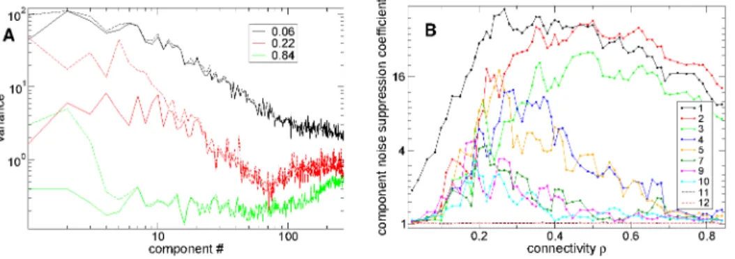
In Figure 9(a) we show PSTH variance (dashed lines) and PSTH noise (solid lines) versus component number for the three different network simulations of different connectivity investigat-ed in Figure 8. At interminvestigat-ediate connectivity, r~0:22, PSTH noise (solid red) is significantly suppressed below PSTH variance (dashed red) up to about component#10. On the other hand at high connectivityr~0:84(green) only the first three components show suppressed noise while at low connectivity,r~0:06, (black) little noise suppression is evident for any components except the first.
To quantify noise suppression in Figure 9(b) we show the ratio of PSTH variance to noise variance versus connectivity for several components. At high connectivity this quantity is large for only the first three components while as connectivity decreases more and more components start to show considerable noise suppression. The higher the component the greater the noise suppression in general. At connectivity around r~0:2, 10 components show noise suppression. Interestingly there appears to be quite a sudden transition from high noise suppression to low noise suppression around component number10. Noise suppression weakens again as connectivity decreases further however. Again the peak of noise suppression in most components occurs in the transition regime close to the striatally relevant connectivity region.
Discussion
In this paper we investigate how a minimalistic model of a local striatal MSN network responds to variations in cortical driving.
We first illustrate using a spike raster plot and mean similarity matrix that the MSN network model can display cell assembly population dynamics locked to stimulus onset times, as previously demonstrated in [29]. We next investigate under what network conditions the reproducibility of stimulus onset locked dynamical evolution across repeat presentations of a given stimulus is maximized and for how long the reproducible patterns persist after stimulus onset. To this end we analyse how 500 cell networks respond to temporally varying cortical driving using a2|2second input switching protocol. As discussed in the model section MSN networks of size 500 with connectivity around0:17and IPSP sizes around200*300mVprovide a reasonable representation of real local MSN network connection structure. By varying parameters individually, so that other factors are kept constant, around this striatally relevant regime we show that dynamical evolution is significantly reproducible for up to about a second after stimulus onset, but, remarkably, only at striatally relevant connection probability and IPSP size. These behaviourally relevant time scales are much longer than any represented in the model parameters. Dynamical evolution is most reproducible soon after stimulus onset and decays thereafter. Outside the striatally relevant parameter range reproducibility is much weaker for all epochs after stimulus onset.
We also investigate how stimulus distinguishability depends on IPSP size. Soon after stimulus onset the current stimulus is only weakly distinguishable from the previous one for all connection strengths. Distinguishably increases with time elapsed from
Figure 9. Ratio of signal to noise variance maximal at striatal connectivity in first 10 principal population components. (a) Component PSTH variance (dashed) and noise variance (solid) versus component number for three simulations of different connectivityr(see key) corresponding to Figure 8 with the same parameters. (b) Ratio of signal variance to noise variance for several components (see key) versus connectivityr. Peak synaptic conductance varies as3:4=(50r)nSand peak IPSP size as&(50=r)mV. (a,b) 500 cell network simulations of 168 seconds
stimulus onset. Most remarkably we find that the background activity (at long times after stimulus onset) generated by different stimuli shows a maximal distinguishability and this maximum occurs at striatally relevant IPSP size. In the striatally relevant parameter regime stimulus distinguishability takes about a second after stimulus onset to saturate at its maximal value.
To shed light on the origin of these optimal properties we investigate how the network generated dynamical activity of 500 cell network simulations under constant (fluctuating) excitatory drive, without input switching, depends on connectivity and connection strength. We find a transition in network generated dynamical activity around 17% connectivity. At connectivity greater than this we find a winners-take-all like regime where some cells fire fairly regularly and the rest are quiescent. On the other hand at lower connectivities we find that most cells participate in network activity but fire in a very bursty way. We also find that the MSN network under constant (fluctuating) excitatory drive shows a connection strength dependent transition when IPSPs have size around 200*300mV, also separating a winners-take-all like regime from a regime where most cells are actively burst firing. Interestingly in both transitions the proportion of active cells shows a minimum, approximately50%, close to where the mean cell CV crosses unity. Most remarkably both transitions occur in the striatally relevant parameter range. CVs somewhat greater than unity are also commonly observed for MSN cells [13,15,26] and our results are thus in good agreement with observations.
To understand the network transition in more detail we investigate a simplified deterministic model of the network rate dynamics with parameters set exactly as in the full model. We are able to accurately reproduce the connectivity and connection strength dependence of network statistical quantities as well as the transition at striatally relevant parameter settings. We also numerically compute the maximal Lyapunov exponent and show that the network is marginally stable at striatally relevant parameter settings, separating a chaotic from a stable regime. In the stable regime the vast majority of network simulations show fixed point dynamics, especially at high connectivity, (see Supplemental Text S1). However at lower connectivity in the stable regime just above the transition to chaos some simulations display periodic dynamics. These interesting transitions will be the subject of future studies.
There are quantitative differences in the behaviour of the relative entropy and proportion of active cells between the rate and spiking models however. This is mainly due to the absence of dynamical effects induced by the spiking. Spiking causes noisy fluctuations around the fixed point states which reduces the relative entropy and may affect stability of attractors in the rate model. The periodic dynamical states are less likely to be observed in the full spiking network. Also transient periods of spike phase locking which may occur in the full spiking model [44] are absent in the rate model. Differences also result from approximating the firing rate dependence of the conductance based synapses by a fixed value (see Methods), and from the absence of noise in the excitatory driving.
We next ask whether stimulus onset locked reproducible dynamics is mediated by single cells or by MSN cell assemblies with coherent slowly varying rates. To investigate this we apply principal component analysis to firing rate time series generated using a long 100 msec time window. Temporal variation in principal components is generated by the coherent activity of populations of cells. We show that at high connectivity only the first three population components show strong dependence on cortical variations. The first component represents the winning set of cells while the next two only activate transiently at stimulus
switches. Network dynamics appears very stable and activated components rapidly relax between two fixed point states, one for each stimulus, characterised by different stimulus dependent distributions of regularly firing and quiescent cells across the network. As connectivity decreases more and more population components display reproducible dynamics after stimulus switches, peaking at around 10 at striatally relevant connectivity. The temporal variations of these components are generated by the coherent activation and deactivation of different subpopulations of cells which inhibit and disinhibit each other. At connectivities near the transition the network successively visits different transient distributions of active and quiescent cells before eventually finding a stable distribution. As connectivity decreases further population components appear to become unstable, wandering apparently randomly without locking to stimulus onset times. Thus cortical driving interacts maximally with network generated population activity at striatally relevant connectivity.
Now we discuss how these results can be explained within the framework of dynamical systems theory. There have been many investigations of dynamical regime transitions in networks of excitatory and inhibitory neurons. Regimes of synchronous and asynchronous irregular activity as well as oscillatory regimes have been found [45–48]. Sompolinsky et al. [49] found a transition from a stationary phase to a chaotic phase in a network of nonlinear elements interacting via random asymmetric couplings. The random firing activity in the asynchronous regime was shown to be generated by chaos produced by the quenched random network structure. The transition from synchronous to asynchro-nous activity which occurs when the network balance changes from excitatory to inhibitory is accompanied by a sudden transition in ISI CV from a value close to zero to one much larger than unity. However these studies treat a network in the limit of sparse connectivity rvv1 so that correlations in
fluctuations in input a cell receives can be neglected. In this sparse limit the inputs to each cell from the rest of the network are described by a single common time varying firing rate. The calculations do not apply when significant correlations appear beyond those induced by this common rate. The network studied here with r&0:2 is far from this limit. Indeed we specifically investigate the dynamical switching of cell assemblies [26] which are groups of transiently strongly correlated cells. Moreover different cells have very different temporal modulations of their firing rates. However our results, in particular the fact that CV values are close to unity, so that spiking activity is Poissonian, and the fact that50%of the network is active in the transition regime, suggest that the network may be close to balanced in the transition regime.
dynamics depending on the connectivity matrix. The present work extends this study to a random inhibitory network modeling the striatal MSN network and investigates its behaviour under variation of connectivity and connection strength. Performance has been shown to be optimal in the marginally stable state known as the ‘edge of chaos’ in several studies of networks which exhibit a transition from stable to chaotic dynamics [36–39]. In recent work Toyoizumi and Abbott [37] determine analytically that the signal-to-noise ratio of large randomly connected networks diverges in a critical state near the edge of chaos, and the memory lifetime of the network also diverges. In fact they find performance is optimal in the chaotic regime close to the transition.
Here we offer the following rough explanatory scenario. Our simulations of the deterministic reduced rate network suggest that the phenomenon we observe here is related to ‘critical slowing down’ occuring in marginally stable weakly chaotic transient dynamics close to the edge of chaos. Indeed (at least) two factors seem relevant for the generation of complex reproducible dynamics in the present random network model under the periodic forcing of the stimulus switching. First the dynamical trajectories generated by the network dynamics should remain quite complex and high dimensional for long periods after stimulus onset. If this is not the case multiple different states in a sequence cannot be discriminated or the elapsed time represented in this random network model. Second network dynamics in the periodically forced system should be stable with period of the forcing stimulus. The stability of dynamics under periodic forcing depends of course on the stability of dynamics generated by the autonomous network in both the stimuli in the absence of forcing. However it also depends on other factors such as the period of the forcing stimulus. In general periodic driving can cause stable activity states to become chaotic and vice-versa. Indeed Rajan et al. [42] have recently shown that periodic forcing can suppress neural network generated chaotic dynamics in a frequency dependent way. They also show suppression of chaotic activity depends on the strength of the forcing.
One way in which activity in the transition regime between stable and unstable behaviour can be both complex and reproducible is due to temporally extended activity which would be transient to a stable fixed point in the unforced system. Indeed deep in the winners-take-all regime, far from the transition, network activity in the unforced system is characterised by a very stable stimulus dependent fixed point. In the periodically forced system after the excitatory input is switched the system moves to a new fixed point. The system moves rapidly between the fixed points due to their strong stability and with a highly reproducible trajectory due to the consistency of initial state across repeat stimulus presentations. Reproducibility is reflected in the strong noise suppression seen in all activated components (Figure 8(a)), but only three components are activated and only briefly. Thus dynamical evolution is highly reproducible but low dimensional and short lived. As the transition is approached from the winners-take-all regime by varying the network parameters the fixed points become less stable and the system takes longer to relax to the new fixed point after the stimulus is switched, lingering in the vicinity of the old fixed point. This dynamical slowing near the transition can generate complex transients on timescales much longer than those represented in the model parameters. Thus for extended transient periods after stimulus onset firing activity resembles the previous stimulus. Indeed in our simulations stimulus distinguishability increases with time elapsed after a stimulus switch.
On the other hand deep in the unstable regime reproducible stimulus locked dynamics does not occur even in the completely deterministic reduced rate network simulations (data not shown.)
Here dynamical activity is complex and high dimensional, requiring many principal components to explain is variance, and thus can easily generate a sequence of strongly differing states. However since nearby trajectories rapidly diverge the network activity state at stimulus onset is strongly varying across repeat presentations and reproducibility is lost.
Transient activity in the unforced system may be complex and higher dimensional close to the transition due to the proximity of periodic and chaotic states and the prescence of attractor ruins. Attractor ruins are regions of phase space where attractors are weakly destabilized and close to which the flow is still very slow [54]. Indeed in the deterministic simulations of the reduced rate network we also find stable periodic states, limit cycles (torii), as well as chaotic states in the transition regime (see Supplemental Text S1), suggesting the proximity of Hopf bifurcations. In this case transients initiated after stimulus changes may decay to the new fixed point in an oscillatory fashion. Indeed the particular example of principal component time series shown Figure 8(e), in the transition regime, may indicate persistent oscillatory waves of inhibition and disinhibition between cell populations. More complex scenarios include slow switching along sequences of metastable ‘saddle-sets’ via heteroclinic channels, as has been shown to occur in asymmetrically coupled inhibitory rate networks (like the reduced rate network studied here) by Rabinovich and coworkers [55,56] in the paradigm of winnerless competition. Here the trajectory remains in the vicinity of a metastable saddle-set for an extended period before suddenly moving off to the next one. Saddle-set states may be fixed point like, corresponding to firing rate cell assemblies, particular transient short-lived distribu-tions of active and quiescent cells, or more complex dynamical attractor ruins. Rabinovich et al. [56] also demonstrate that this scenario can be preserved even in the presence of noise. Deco and coworkers [57,58] have also studied switching between ‘ghost attractors’ in a critical regime near a transition to a multistable state. However besides transient activity we should also mention that in the transition regime activity generated by one stimulus may be chaotic while in the other stable fixed point thus the periodically forced activity will be stable but complex. In general we suggest the MSN network is in a marginally stable regime facilitating the generation of weakly chaotic and complex transient activity. When the network is periodically forced by the stimulus switching this activity can produce complex but stable periodic activity.
This scenario is consistent with the observation that the transition seems to occur when the network is just balanced, as discussed above. In the winners-take-all state the permanent quiescent component allows the remaining active cells to fire fairly regularly, thus reducing the mean CVv1, while in the chaotic
switching state the transient activation of sets of cells in assemblies produces the highly bursty CVw1 values. The transition thus
occurs whenCV*1. That this transition happens to occur in the striatally relevant parameter regime is non-trivial and unexpected. Suggestions of critical dynamics can be seen in the the PSD of the higher components in the intermediate (Figure 8(d)) and low (Figure 8(f)) connectivity simulations. These display a region of rapid growth in the range1*10Hz which appears approximately linear in the log-log plot, so thatPSD(f)*1=fk, wherekw0. PSD
is evidence of fractal self-similar dynamical behaviour over this range of time scales. It should be remembered however that the PSD we calculate here are for principal components not single cells, and thus represent aggregate fluctuations of many cells. Nevertheless similar results are observed for single cells (data not shown.)
Indeed we observe (Figure 8(b,d,f)) that the slope of the power-law of the PSD of the highest components in this frequency range, 1*10Hz, increases with decreasing connectivity. At low connec-tivity slopes exceed two, kw2, (data not shown). If power-law
scaling is present on all timescales a slope ofk~2is consistent with Brownian motion. Our PSD results at low connectivity, where
kw2, suggest that the higher components behave ‘locally’ (on
short timescales) like random walks [62], so that the expected size
of component fluctuations across an interval of time
SDx(t2){x(t1)DT increases with the time interval Dt~t2{t1 for intermediate timescales Dt&0:1{1secs, before saturating at a constant level for longer time scales, as shown by the saturation of the PSD at low frequencies. This is also consistent with our observation of chaos (which generates fractal dynamical trajecto-ries) [62,63] in the rate dynamics at low connectivities. At high connectivity we find slopes k&0 indicating a white noise like process. This is consistent with the observation of stable fixed point like rate dynamics decorated by high frequency fluctuations generated by random spike arrival times. At striatally relevant connectivities slopeskare close to 1 (data not shown) as in [59] (Figure 8(a)). Although there are various origins of1=f noise [61], it has been associated with criticality [64] and thus our PSD results may also be consistent with the scenario of critical slow dynamics near a transition.
Neural activity has often been modeled as a marginally stable critical process. Usually this is based on spiking activity. For example in a ‘critical branching process’ [65–67] spiking activity ‘just propagates’ across a network without exploding or dying, but slower rate variations can also be marginally stable [37,50]. Since the dynamics is between a stable pattern of activity and random behavior spatiotemporal activity is highly susceptible to perturba-tions and the macroscopic behaviour of large cell populaperturba-tions can be affected by small events. Even though interactions are only local critical systems develop correlations which extend over large temporal and spatial scales compared with the scales represented in the system parameters. These characteristics make make criticality an attractive scenario to embed neural information processing.
We have shown that in the vicinity of the transition the network displays optimal properties. A variety of optimal properties have been associated with marginally stable and critical behaviour in neural systems [68,69]. It has been suggested to optimize information transmission [70–73], sensitivity to sensory stimuli and dynamic range [50,74], or memory size and computational abilities [38]. Critical and metastable dynamics [75] can also facilitate rapid adaptation to changes in processing demands [60,76–80]. Self-organized critical systems include mechanisms to maintain themselves in the critical state [60,64]. In a similar way the MSN network may remain critical by dynamically self-regulating its properties, through growth, pruning or plasticity [33,81,82], for example.
Chaotic balanced networks [46,83] are thought to be respon-sible for the irregular bursty activity which has often been observed throughout the brain [84–87]. Furthermore neuronal variability is also often observed to be task dependent [84–91]. A sudden reduction in firing variability after stimulus onset has been observed in several recent studies [92–97]. Although there is no striatal study available our results of noise suppression after
stimulus onset, previously reported in Ponzi and Wickens [98], are in good agreement with these studies.
Manyin-vivobehavioural studies, in particular of reinforcement learning and temporal credit assignment tasks, show that coherent slowly varying activity in cortico-BG microcircuits is important in the encoding of movement [2,15,99–103] and the execution of learned motor programs and sequence learning [1,104–114]. The quantities we chose to investigate here, the reproducibility of stimulus onset locked activity and stimulus distinguishability, are both highly relevant for such tasks. Our cortical input switching protocol, although it is the simplest conceivable, may still approximate the sudden stimulus changes which occur in such tasks. Such stimuli changes include the sudden appearance of visual cues typical in primate studies and sharp onset auditory tones in rodent maze tasks. The spatio-temporal dynamics [55,56,69,115–120] generated by this network could be utilized in such behavioural tasks or in ‘reservoir computing’ style cognitive processing [27,38,39,55,121,122]. In particular since network activity generates a diverse set of both stimulus and temporally specific cell responses [27,123–125] it could be useful to provide fluctuations at specific times after a specific behavioural event, necessary to facilitate exploration of both sensory input and motor response [126–129] or simply to drive temporally delayed motor response or to control the timing of a dopamine signal in temporally delayed reinforcement learning.
In agreement with this work a variety of diverse response profiles with phasic activity peaks covering a wide spectrum of delays after task events has been observed in such tasks [8–10]. Jin et al. [8] found MSNs with responses so diverse that they suggested the cells could have encoded time as a population, even though the animals were performing a simple task that did not have precise-timing requirements. The authors concluded that their results could not be accounted for by a distribution of response latencies to visual inputs. They suggested additional mechanisms were needed to generate the observed response profiles, which had timescales much longer than the visual response range, and that the brain may intrinsically have properties for forming the basis of temporal computations even when not needed by the task.
Recently Adler et al. [13] addressed whether MSN activity is internally generated within the striatum, or whether it is driven by cortex. They found MSN cell assemblies which were activated at different latencies after cue presentation in a behavioural task. The cell assemblies were not differentiated by intrinsic MSN cell properties, nor were such assemblies found for the other striatal cell types investigated. For example the tonically active interneu-rons activated rapidly on cue presentation without distinct clustering, while clusters of globus palidus cells also did not show different activation latencies. The authors suggested that the sequential MSN cell assembly activations could be a result of MSN network dynamics. Here we show that such activity could in principle be generated internally by the MSN network and furthermore that cortical input may be transformed by the striatum in a complex way.