Estimation Techniques for Monitoring and Controlling the Performance of the Computer Communication Networks

ISSN 1546-9239

© 2005 Science Publications

Corresponding Author: Ibrahiem M. M. El Emary, Amman Al Ahliyya University, Amman, Jordan

Estimation Techniques for Monitoring and Controlling

the Performance of the Computer Communication Networks

1

Ibrahiem M.M. El Emary and

Adanan I. Al Rabia

1

Amman Al Ahliyya University, Amman, Jordan

2

Al Balqa Applied University, Al Salt, Jordan

Abstract: This study was concerned with making a comparative study between four types of time series model with the goal of choosing the optimum one to predict the performance of a computer communication network. The investigated four types of time series are: Least Square (LS), Fourier series, Exponential Weighted Moving Average (EWMA) and the Auto Regressive Integrated Moving Average (ARIMA). Comparative study is based on comparing some of statistical measurement for these four time series models as: mean standard deviation and variance. We apply these various types of time series on two types of network to predict their performance; the first one is called token bus while the second one is called the token ring. Concluded results prove that both EWMA and ARIMA perform better than the others LS and Fourier since both EWMA and ARIMA forecast the network performance parameters with an accuracy of 98% near the actual values.

Key words: Exponential weighted moving average, auto regressive integrated moving average, least square, relative error, standard deviation

INTRODUCTION

Computer communication networks require monitoring to detect performance anomalies, but problem detection and diagnosis is a complex task requiring skilled attention. Although human attention was never ideal for this task, as networks of computers grows larger and their interactions more complex, it falls far short. Existing computer-aided management systems require the administrator manually to specify fixed '' trouble'' thresholds.

The process of managing a system performance is an iterative one performed by a human, the steps involved might not be as well-defined as described here, but the basic iterative steps still exist. The performance management process is composed of a definition phase, a diagnostic phase and a therapy phase. The definition phase consists of determining what performance criteria are to be evaluated and how the data will be collected and analyzed. Diagnosis begins by making measurements of the system. This in followed by analysis of the collected data. Analysis is done manually or with assistance from another computer. During analysis, the performance is recognized and categorized. After the analysis, if the results suggest that some improvements in performance are possible, a therapy phase is beginning. During this phase, adjustments to the system are made in an attempt to alleviate the problem. The remaining phases are repeated until there are no known performance problems in the system.

This study describes a time series modeling technique that can be used for more automatically

detecting the problems of computer network performance. Techniques that are used are based on four types: EWMA, LS, FOURIER and ARIMA, they allow detection of performance problems in a computer network by providing a means of detecting performance criteria values that are out of normal range

Our effort in this study was focused on making a comparative study between these four types of time series in order to select the optimal one and use it in the management process. The comparative studies depend on using some of statistical criteria as: Mean, standard deviation and variance. Numerical results show that EWMA is the optimum type of time series models since it can forecast or predict the network performance with accuracy approximately equal to 98% of the actual values. According to this output result, network an administrator can use this approach to monitor the network performance and decide if there is a problem or not.

The basic form of the seasonal time series model is written as:

Xt=b1+b2t+Ct+€t (1)

Where:

b1: A constant component.

b2: A trend component

Ct: A seasonal factor

€t : A random error component

The effect of the seasonal factors Ct is to

de-seasonalize the current reading X. The length of the seasonal variation is fixed at length L. The parameters b1, b2 and Ct, t=1, 2… L must be estimated. These

estimates are updated at the end of each period. The model adapts to changes in the data by the use of three smoothing constants α β, ,andγ.the α β, , and γ smoothing constants are used to smooth the: constant, trend and seasonal components of the time series model[2].

The estimates b1^, b2^, and ct^, t=1… L is computed

as follows:

b1^ (t)= α[Xt-ct ^ (t-L)]+(1-α) [b1^(t-1) + b2^(t-1)] (2)

b2 ^

(t)= ß [b1 ^

(t) - b1 ^

(t-1)] + (1-ß) [b2 ^

(t-1)] (3) Ct

^

(t) = γ [Xt - b1 ^

(t)] + (1-γ ) [ct ^

(t-L)] (4)

Where, 0< α_,ß,γ _<1

Autoregressive integrated moving average time series model (ARIMA): ARIMA is based on finding a model that accurately represents the past and future patterns of a time series[1]:

Yt = Pattern + et (5)

Where:

Yt = The forecasting value

et = A random error

The pattern can be random, seasonal, trend, or a combination of them.

ARIMA model building methods use a simple, versatile model notation; they are designated by the level of auto regression, integration, and moving averages. This standard notation identifies the orders of auto regression by p, integration or differencing by d, and moving average by q.

Auto regression which is called an ARIMA (1, 0, and 0) or AR (1) is represented by:

Yt = θ0 + Φ1 Yt-1+et (6)

where, θ0 and Φ1 are coefficients chosen to minimize

the sum of squared errors.

Fig. 1: Idea of least square Yt : The forecasting value

et: A random error

Moving average which called an ARIMA (0,0,1) or MA (1), is represented by:

Yt = µ - θ0 et-1 +et (7)

Where:

Yt: The forecasting value

θ0: An estimated coefficient

et: A random error

Integrated series which called and ARIMA (0,1,0) is represented by:

Yt = Yt -1 +et (8)

Where:

Yt: The forecasting value of time t

Yt-1: The forecasting value at time t-1

et: A random error

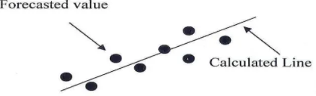
Least square time series model (LS): Least Square (LS) is another example of the time series models. The idea of the least square method is to find a line which goes through all points and be close as possible to each one of points as shown in the Fig. 1.

The line equation that represents LS is given by[1]:

Y=mX+b (9)

Where:

Y: Forecasted values on y axis X: Value of time on x axis

So, we must find the line equation with minimum ε which is the error square sum i.e.:

t t

2 2

i i

i 0 i 0

(y y) (y (mX b))

= =

=

∑

∑

ε (10)

where, yi: the forecasted value of time i.

from 0 to n. When we determine the derivatives of two parameters m and b, we get:

n n n n

i 0 i 0 i 0 i 0

2 2

m n( xy) ( y) / n( x) ( x)

= − = =

=

∑

∑

∑

∑

n n

i 0 i 0

b [( y / n] m[( x) / n]

= =

=

∑

∑

Where: b: Constant

y: Forecasted values on y-axis X: Values of time on x-axis m: Line slope

n: Period of time

Fourier time series model: The fourth series type that we are studying of the Fourier series. The Fourier series is the series of the form[3]:

Xt=A0+

n 1

∞

=

∑

The constants A0, An and Bn are called the

coefficients of F n(x).

Where: i = 0, 1 … n A0 = 1/n

n 1

t 0

−

=

∑

An = 2/n

n 1

t 0

−

=

∑

Bn = 2/n

n 1

t 0

−

=

∑

Where:

Xt: The predicted value

t: The time of forecasting Wj: The frequency

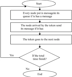
Descriptions of the simulated computer networks: In this section, we deal with two types of computer networks which are simulated according to Fig. 2. Their performance was tested by the previous four types of time series model. The first one is called a token ring computer network, while the second one is called a token bus. The ring topology is a physical, closed loop consisting of point-to-point links. Each node on the ring acts as a repeater. It receives a transmission from the previous node and amplifies it before passing it on. A token ring network was a special frame called a token that rotates around the ring when no stations are actively sending information. When a station wants to transmit on the ring, it must capture this token frame.

Fig. 2: Flowchart of operation for a token ring computer network

Fig. 3: Flowchart illustrating the operation of a token bus network

The owner of the token is the only station that can transmit on the ring. A flowchart that illustrates the operation of a token ring computer network is shown in Fig. 2[4].

On the other hand, in a token bus network, all devices are attached to the same transmission medium. A flowchart that illustrates the complete concept of token bus operation is shown in Fig. 3.

communication network. This simulator produces a data for: network utilization, network delay, network collision frequency, each node collision frequency, and each node delay. These data are saved into a file where this experiment takes the first half amount of data for training and the remaining half used for testing. The experiment produced forecasted data for network utilization, network delay, network collision frequency, each node collision frequency, and each node delay from the actual data had been entered before. The data taken passed through four time series models where each one produced a separate different forecasting data to a different file. Figure 4 shows the standard deviation of the bus busy time for the token bus computer network using four types of time series models. From the Figure, we see that the ARIMA and EWMA standard deviation are close to zero because the predicted value close to the actual values, while the LS and Fourier far. Figure 5 shows the relative error of the bus busy time for the token bus computer network using four types of time series models. From the Figure, we see that the ARIMA and EWMA relative error is too small since the predicted value is close to the actual values, while the Fourier relative error is large relatively.

Fig. 4: Standard Deviation of bus busy time for the token bus network using four types of time series models

Fig. 5: Relative Error of bus busy time for the token bus network using four types of the series models

Figure 6 shows the standard deviation of network delay for the token bus computer network using four types of time series models. From the Figure, we see that the ARIMA and EWMA standard deviation are close to zero because the predicted value close to the actual values, while the LS and Fourier far.

Figure 7 shows the relative error of the network delay for the token bus computer network using four types of time series models. From the Figure, it is seen that the ARIMA and EWMA relative error is too small since the predicted value close to the actual values, while the Fourier relative error is relatively large.

Figure 8 shows the standard deviation of the utilization of the token ring computer network using four types of time series models. From the Figure, we see that the ARIMA and EWMA standard deviation are close to zero while the LS and Fourier far.

Figure 9 depicts the relative error of the utilization of the token ring computer network using four types of time series models. . From the Figure, we see that the ARIMA and EWMA relative error is too small while the Fourier relative error is huge relatively.

Figure 10 shows the standard deviation of the delay for node 0 token bus computer network using four types of time series models. From the Figure, we see that the ARIMA and EWMA standard deviation are close to zero.

Fig. 6: Standard deviation of the network delay for the token bus computer network using four types time series models

Fig. 8: Standard deviation of the utilization of the token ring computer network using four types of the series models.

Fig. 9: Relative error of the Utilization of the token ring computer network using four types of the time series models

Fig. 10: Standard deviation of delay for node 0 token bus computer network using four types of time series models

Figure 11 depicts the relative error of the delay for need 0 token bus computer network using four types of time series models. From the Figure, we see that the ARIMA and EWMA relative error is too small while the Fourier relative error is relatively large.

Figure 12 shows the Standard deviation of the collision frequency of the token bus computer network using four types of time series models. From the Figure, we see that the ARIMA and EWMA standard deviation are close to zero while the LS and Fourier far.

Fig. 11: Relative error of delay for node 0 token bus computer network using four types of time series models

Fig. 12: Standard deviation of the collision frequency of the token bus computer network using four types of time series models

Fig. 13: Relative error of the collision frequency of the token bus computer network using four types of time series models

Figure 13 shows the relative error of the collision frequency of the token bus computer network using four types of time series models.

From the figure we can see that the ARIMA and EWMA relative error is too small while the Fourier relative error is relatively large.

seasonal, and random. In EWMA, the constant which is always presented have the biggest effects to the total result of EWMA and updated periodically while the other components have small effect on the result. So, it goes through a steady state.

ARIMA consist of three models AR, I, and MA, each one computes one parameter and passed it to the next one. The change of actual values will affect on the ARIMA result time. LS is a line equation method which tries to find the slope and constant of the line equation that goes through the most of historical points. So, it will be affected by the far points in history. Finally, because the Fourier time series model has periodically shape, it will take the waveform and still progress over time as its start. In all models, the value factors affect the result of the time series and give those closest between them.

CONCLUSION AND FUTURE WORKS

In this work, we monitor the performance of both token ring and a token bus computer network. Any failure of network component will affect one of the network measurements (Utilization, system delay, total channel busy time … etc..). If we know about abnormal changing in these measurements, this means that there is some problem in the network. We compare between four time series models (ARIMA, EWMA, LS, and Fourier) in order to choose the optimal one for estimating the performance of the above two types of computer networks. We found that the EWMA time series is the best one, next the ARIMA with small differences between them. This conclusion has been obtained as a result of making a statistical comparison between these four types of time series models.

As a future work, we suggest to use the EWMA time series model in building an Expert system can assist in putting a threshold value of the network performance parameters instead of putting it manually by the network administrator. Here the accuracy of management and administration will be raised to a noticeable level which can be reflected in raising the performance of a computer communication networks.

REFERENCES

1. Ahmad, B.H., 2005. On the application of time series models for detecting the problems of computer communication networks. Al-Balqa’ Applied University- Jordan, Master Thesis. 2. William, S., 2003. Cryptography and Network

Security Principles and Practice. 3rd Edn., Pearson Education International.

3. Malandain, E. and P. Skarek, An Expert System for Accelerator Fault Diagnosis.

4. William, S., 2004. Data and Computer Communications. 7th Edn. Pearson Education International.

5. William, S., 2002. High-speed networks and internets: Performance and quality of service. 2nd Edn., Prentice Hall.