ACPD
13, 25801–25825, 2013Removing discontinuities in
ERA-Interim temperatures
C. McLandress et al.
Title Page
Abstract Introduction
Conclusions References
Tables Figures
◭ ◮
◭ ◮
Back Close
Full Screen / Esc
Printer-friendly Version Interactive Discussion
Discussion
P
a
per
|
D
iscussion
P
a
per
|
Discussion
P
a
per
|
Discuss
ion
P
a
per
|
Atmos. Chem. Phys. Discuss., 13, 25801–25825, 2013 www.atmos-chem-phys-discuss.net/13/25801/2013/ doi:10.5194/acpd-13-25801-2013
© Author(s) 2013. CC Attribution 3.0 License.
Atmospheric Chemistry and Physics
Open Access
Discussions
This discussion paper is/has been under review for the journal Atmospheric Chemistry and Physics (ACP). Please refer to the corresponding final paper in ACP if available.
Technical Note: A simple procedure for
removing temporal discontinuities in
ERA-Interim upper stratospheric
temperatures for use in nudged
chemistry-climate model simulations
C. McLandress1, D. A. Plummer2, and T. G. Shepherd3
1
Department of Physics, University of Toronto, Toronto, Ontario, Canada
2
Canadian Centre for Climate Modelling and Analysis, Victoria, British Columbia, Canada
3
Department of Meteorology, University of Reading, Reading, Berkshire, UK
Received: 25 July 2013 – Accepted: 20 September 2013 – Published: 8 October 2013
Correspondence to: C. McLandress ([email protected])
ACPD
13, 25801–25825, 2013Removing discontinuities in
ERA-Interim temperatures
C. McLandress et al.
Title Page
Abstract Introduction
Conclusions References
Tables Figures
◭ ◮
◭ ◮
Back Close
Full Screen / Esc
Printer-friendly Version Interactive Discussion
Discussion
P
a
per
|
D
iscussion
P
a
per
|
Discussion
P
a
per
|
Discuss
ion
P
a
per
|
Abstract
This note describes a simple procedure for removing unphysical temporal discontinu-ities in ERA-Interim upper stratospheric temperatures in March 1985 and August 1998 that have arisen due to changes in satellite radiance data used in the assimilation. The derived adjustments (offsets) to the global mean temperatures are suitable for
5
use in chemistry-climate models that are nudged to ERA-Interim winds and tempera-tures. Simulations using a nudged version of the Canadian Middle Atmosphere Model (CMAM) show that the inclusion of the temperature adjustments produces tempera-ture time series that are devoid of the large jumps in 1985 and 1998. Due to its strong temperature dependence, the simulated upper stratospheric ozone is also shown to
10
vary smoothly in time, unlike in a nudged simulation without the adjustments where abrupt changes in ozone occur at the times of the temperature jumps. While the ad-justments to the ERA-Interim temperatures remove significant artefacts in the nudged CMAM simulation, spurious transient effects that arise due to water vapour and persist for about five years after the 1979 switch to ERA-Interim data are identified, underlining
15
the need for caution when analysing trends in runs nudged to reanalyses.
1 Introduction
Stratosphere-resolving chemistry-climate models (CCMs) are powerful tools for sim-ulating and understanding the impacts of ozone depletion/recovery and increasing greenhouse gas emissions on the climate system and for predicting its future changes.
20
However, because free-running CCMs are unable to reproduce the observed meteo-rology, the simulated fields cannot be compared to observations on a day-to-day basis. Furthermore, biases in one model variable can have knock-on effects on other vari-ables. For example, a bias in temperature in the upper stratosphere (due to a missing process in a model’s radiative transfer scheme) can impact on chemistry, thus causing
25
a bias in another variable such as ozone, even if the chemistry scheme were perfect.
ACPD
13, 25801–25825, 2013Removing discontinuities in
ERA-Interim temperatures
C. McLandress et al.
Title Page
Abstract Introduction
Conclusions References
Tables Figures
◭ ◮
◭ ◮
Back Close
Full Screen / Esc
Printer-friendly Version Interactive Discussion
Discussion
P
a
per
|
D
iscussion
P
a
per
|
Discussion
P
a
per
|
Discuss
ion
P
a
per
|
Recently, there has been a concerted effort to nudge (or relax) CCMs to the horizon-tal winds and temperatures from reanalyses. Constraining the dynamical fields to follow the observations through nudging enables day-to-day comparisons of other model vari-ables to observations to be made and biases in the model “physics” and chemistry to be identified. To this end the International Global Atmospheric Chemistry (IGAC) and
5
Stratospheric Processes And their Role in Climate (SPARC) Chemistry-Climate Model Initiative (CCMI) has proposed a set of specified-dynamics simulations in which the CCMs are nudged to reanalysis datasets from 1980 to 2010 (Eyring et al., 2013). The proposed REF-C1SD nudged simulations will be used for upcoming ozone and climate assessments.
10
This approach inherently relies on the reanalysis used to do the nudging not contain-ing spurious temporal inhomogeneities. This is a challenge for reanalyses because of the inhomogeneous nature of the observations. The reanalysis centres have made ma-jor advances in dealing with these issues through bias correction, with the European Centre for Medium-Range Weather Forecasts (ECMWF) “Interim” Reanalysis
(ERA-15
Interim; Dee et al., 2011) being the first reanalysis to use fully automated variational bias corrections of satellite observations. However, bias correction relies on having mul-tiple data sets, in particular “anchoring” data sets such as radiosondes. Unfortunately, in the upper stratosphere, where there is only one source of long-term temperature data (operational nadir-viewing satellites), bias correction cannot be effectively applied
20
if, as in the case of ERA-Interim, model bias is large and adjustment towards a biased model state is to be avoided. Dee and Uppala (2008) discuss the difficulties associated with assimilating radiances from the Stratospheric Sounding Unit (SSU) and the Ad-vanced Microwave Sounding Unit (AMSU-A). They show that the transition from SSU to AMSU-A data in August 1998 introduces large global-mean temperature increments
25
ACPD
13, 25801–25825, 2013Removing discontinuities in
ERA-Interim temperatures
C. McLandress et al.
Title Page
Abstract Introduction
Conclusions References
Tables Figures
◭ ◮
◭ ◮
Back Close
Full Screen / Esc
Printer-friendly Version Interactive Discussion
Discussion
P
a
per
|
D
iscussion
P
a
per
|
Discussion
P
a
per
|
Discuss
ion
P
a
per
|
Here we discuss a simple procedure for removing unphysical temporal discontinuities in ERA-Interim temperature data in the upper stratosphere for use in nudged CCMs. The temperature adjustment proposed here will be useful for high-top CCMs used for the REF-C1SD simulations for CCMI. We apply this procedure to the jump in August 1998 discussed in Dee and Uppala (2008) and also to another large jump in March
5
1985, which was outside of their analysis period. This 1985 jump is due to a change in bias of SSU-3 data from NOAA-9 and subsequent satellites, for which pressure in the instrument’s carbon dioxide cell was higher than on earlier satellites (Kobayashi et al., 2009).
We provide a set of equations and a tabulated set of coefficients that can be easily
10
used to generate the global-mean temperature adjustments. We also provide a link for obtaining data files containing those adjustments. We must stress that our adjustments do not correct the ERA-Interim temperatures, only remove the unphysical temporal discontinuities, which are an artefact of the assimilation process.
We assess the impact of including the temperature adjustments in a nudged
ver-15
sion of the Canadian Middle Atmosphere Model (CMAM). The simulation without the temperature adjustments exhibits large discontinuous changes in global-mean temper-ature in the upper stratosphere, which are absent when the adjustments are applied. The inclusion of the adjustments is shown to have a large impact on the simulated upper stratospheric ozone, which exhibits large jumps contemporaneous with the
tem-20
perature jumps when the unadjusted nudging temperatures are used.
2 Adjusting the ERA-Interim global mean temperatures
This section describes the methodology used for removing the temporal discontinuities (jumps) in the ERA-Interim temperatures in the upper stratosphere. We consider only the global mean since, to a first approximation, it is unaffected by dynamics and is
25
therefore close to radiative equilibrium (e.g. Fomichev, 2009). Since global mean tem-perature varies slowly in time (due to changes in radiative forcing), the jumps can be
ACPD
13, 25801–25825, 2013Removing discontinuities in
ERA-Interim temperatures
C. McLandress et al.
Title Page
Abstract Introduction
Conclusions References
Tables Figures
◭ ◮
◭ ◮
Back Close
Full Screen / Esc
Printer-friendly Version Interactive Discussion
Discussion
P
a
per
|
D
iscussion
P
a
per
|
Discussion
P
a
per
|
Discuss
ion
P
a
per
|
identified in an unambiguous manner. We start by identifying the times at which the jumps occur and then describe the procedure for computing and applying the adjust-ments to the data, which we shall refer to as offsets. The offsets are computed from monthly mean data, but are interpolated to the 6 hourly data that is used to nudge the model.
5
Figure 1 shows global and monthly mean temperature anomaly time series for the top five pressure levels of ERA-Interim. The anomalies are computed with respect to the long-term (1979–2010) monthly means. Superimposed on the overall cooling trend at all levels are large temperature jumps in March 1985 and August 1998, denoted by the thin vertical lines. These are the two jumps that will be removed. The jumps occur
10
simultaneously at all levels, and decrease in magnitude with increasing pressure. The jump in August 1998 results from the switch from SSU to AMSU-A satellite radiances (Dee and Uppala, 2008; Kobayashi et al., 2009). It is not instantaneous, but is spread out over a period of about ten days, as seen by the red curves in Fig. 3b, which shows the 6 hourly data at 1 hPa. The jump in March 1985 exhibits a much different temporal
15
behaviour, for not only is there a shift in the mean value, but there is also a spike just before the jump, as is more clearly seen in Fig. 3a (red curves). This complex temporal behaviour is caused by varying SSU-3 data counts from the NOAA-7 and NOAA-9 instruments, which as noted earlier have different biases, during their several-month overlap period (A. Simmons, personal communication, 2013). There is also a jump in
20
1979 associated with the start of assimilation of SSU-3 data, which we do not attempt to adjust since the ERA-Interim record prior to this time is very short. Figure 1 shows that at 7 hPa the jumps in 1985 and 1998 are not readily distinguished from the geophysical noise. Consequently we shall adjust only the top four pressure levels, namely 1, 2, 3, and 5 hPa. We note that our procedure does not remove possible slow drifts in the
25
reanalysis data that might arise from long-term changes in the satellite data.
ACPD
13, 25801–25825, 2013Removing discontinuities in
ERA-Interim temperatures
C. McLandress et al.
Title Page
Abstract Introduction
Conclusions References
Tables Figures
◭ ◮
◭ ◮
Back Close
Full Screen / Esc
Printer-friendly Version Interactive Discussion
Discussion
P
a
per
|
D
iscussion
P
a
per
|
Discussion
P
a
per
|
Discuss
ion
P
a
per
|
ERA-Interim global mean temperature time series, which differs from the top curve in Fig. 1 in that it includes the annual cycle. These data are deseasonalized by sub-tracting offthe fit to the first four sine and cosine harmonics of the annual cycle. The fits are calculated independently for three time periods, namely 1980 to 1984, 1986 to 1997, and 1999 to 2011, which exclude the years when the jumps occur. The
5
resulting deseasonalized time series is given by the black curve in Fig. 2b. Since the time axis starts in 1980, the jump in 1979 is not seen here. The deseasonal-ized time series is then fit to a function that includes a linear trend, the monthly mean F10.7 solar flux time series recorded by the Geological Survey of Canada (http://www.spaceweather.ca/data-donnee/sol_flux/sx-5-eng.php) and the global mean
10
stratospheric aerosol optical depth time series updated from Sato et al. (1993) as a proxy for volcanic activity (http://data.giss.nasa.gov/modelforce/strataer/). The linear trend accounts for cooling due to the increasing concentrations of CO2 (and, before 1998, ozone loss), while the solar flux term accounts for solar cycle effects, which have a significant impact on upper stratospheric temperatures. The volcanic term is included
15
because it improves the fit, although the upper stratosphere is far from the main region of volcanic influence; omitting the stratospheric aerosol optical depth term has only a minor effect on the values of the offsets. A simpler approach for generating the off -sets would be to compute global mean temperature differences for specific periods before and after the jumps. The problem with that approach, however, is that if the time
20
periods are too long the cooling trend aliases into the average, while if the periods are too short the systematic bias is harder to characterize. Our approach mitigates both of these problems and produces annual mean offsets that yield a smoother transition over the jumps. The fits are computed over the three periods given above, and the time series of the fits are then extended across the years in which the jumps occur. For
25
example, data from January 1980 to December 1984 were used to construct the fit for the first period; the fit was then extended forwards in time to cover 1985. Similarly, the second period was fit using data from January 1986 to December 1997 and the fit was extended backwards in time to cover 1985. The same procedure was used to have the
ACPD
13, 25801–25825, 2013Removing discontinuities in
ERA-Interim temperatures
C. McLandress et al.
Title Page
Abstract Introduction
Conclusions References
Tables Figures
◭ ◮
◭ ◮
Back Close
Full Screen / Esc
Printer-friendly Version Interactive Discussion
Discussion
P
a
per
|
D
iscussion
P
a
per
|
Discussion
P
a
per
|
Discuss
ion
P
a
per
|
second and third periods span 1998. The red curves in Fig. 2b show the fitted data, extended slightly beyond the ends of the data used in computing the fits in order to show the overlap region that is used to calculate the annual mean offsets, which are evaluated at the mid-point of the jump year denoted by the red crosses.
At this stage of the analysis a decision has to be made as to how to apply the offsets.
5
Since there are no independent observations that can be used to validate the global mean temperatures, we will apply the offsets to the first and second time periods, leaving the data after the 1998 jump unchanged. Figure 2c shows the deseasonalized time series with the two annual mean offsets applied, which with the inclusion of the annual cycle yields Fig. 2d. The final step involves the inclusion of the monthly mean
10
offsets. As the post-1998 ERA-Interim data were defined as the absolute reference for the record, seasonal cycle offsets were calculated as the difference between the fitted seasonal cycle of the ERA-Interim monthly temperatures for a particular period and the fitted seasonal cycle for the post-1998 period. The monthly mean offsets for a particular period are then the sum of the seasonal cycle offsets, which by construction have an
15
annual mean of zero, and the annual mean offset calculated from the fitting described above. The final time series with the monthly mean offsets applied is shown in Fig. 2e. Note that the spike in March 1985 remains since there is no way to remove it using our procedure.
The end product of this part of the analysis procedure is two sets of monthly mean
20
offsets for each of the four pressure levels. It now remains to interpolate those offsets to a 6 h grid and to smoothly connect them over the months where the jumps occur. The former is achieved by fitting the monthly mean offsets to the first four harmonics of the annual cycle as follows:
∆T∗
l,n(d)=Cl,n+
4
X
m=1
Aml,ncos
md D
+Blm,nsin
md D
(1)
25
ACPD
13, 25801–25825, 2013Removing discontinuities in
ERA-Interim temperatures
C. McLandress et al.
Title Page
Abstract Introduction
Conclusions References
Tables Figures
◭ ◮
◭ ◮
Back Close
Full Screen / Esc
Printer-friendly Version Interactive Discussion
Discussion
P
a
per
|
D
iscussion
P
a
per
|
Discussion
P
a
per
|
Discuss
ion
P
a
per
|
(1 or 2), andmis the harmonic of the annual cycle. The values of the fit coefficients Aml,n,Blm,n, andCl,n are given in Table 1.
The final step is to smoothly join the 6 hourly offsets for the adjacent periods, be-cause the jump between periods is not instantaneous (see Fig. 3). This is achieved by applying an exponential function of the formEl,n(d)=exp [−(d−dn)/τl,n] where dn
5
is the day of the year of the jump for each period (e.g. d1=80.5 for 12Z 21 March), andτl,n is an e-folding time scale. The latter is specified asτl,1=3 days for all levels,
τl,2=5 days forl=1 hPa, andτl,2=2 days for the remaining levels. These values were
chosen to yield a smooth transition, judged by eye.
Denoting the offsets at level l as ∆Tl, we have for t<t1 (where t is time and t1
10
denotes the first “jump time”, 12Z 21 March 1985) andd is, as before, the day of year:
∆Tl(t)= ∆T∗
l,1(d). (2)
In order to smoothly merge the exponential function that is applied immediately after the first jump with the 6 hourly offsets for the second period we use for t1≤t<t1+
25 days:
15
∆Tl(t)= ∆T∗
l,1(d1)El,1(d)+ ∆T
∗
l,2(d)[1−El,1(d)]. (3)
Fort1+25≤t<t2(wheret2denotes the second jump time, 00Z 1 August 1998):
∆Tl(t)= ∆T∗
l,2(d), (4)
and fort2≤t<t2+25 days:
∆Tl(t)= ∆T ∗
l,2(d2)El,2(d). (5)
20
Finally, fort≥t2+25 days:
∆Tl(t)=0. (6)
ACPD
13, 25801–25825, 2013Removing discontinuities in
ERA-Interim temperatures
C. McLandress et al.
Title Page
Abstract Introduction
Conclusions References
Tables Figures
◭ ◮
◭ ◮
Back Close
Full Screen / Esc
Printer-friendly Version Interactive Discussion
Discussion
P
a
per
|
D
iscussion
P
a
per
|
Discussion
P
a
per
|
Discuss
ion
P
a
per
|
Figure 3, which shows a blow up of the jumps in 1985 and 1998, helps to illustrate the use of the above set of equations. The red curves denote the original 6 h ERA-Interim data at 1 hPa, the blue curves are the adjusted data (i.e. with the offsets ∆Tl added on). The jump timest1andt2are denoted by the left-hand thin vertical lines.
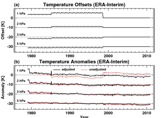
Figure 4a shows the offsets∆Tl at all four pressure levels computed using Eqs. (1)–
5
(6) and monthly averaged for plotting purposes. As expected, the largest component is the annual mean. The corresponding global and monthly mean temperature anomalies with and without the offsets included (the adjusted and unadjusted anomalies, respec-tively) are given by the black and red curves, respectively, in Fig. 4b. The red curves are identical to those shown in Fig. 1.
10
3 Impacts of temperature adjustments in nudged CMAM
3.1 Model description and simulations
The Canadian Middle Atmosphere Model is a chemistry-climate model that extends up to the lower thermosphere (∼100 km). The version used here is nudged to the 6 hourly horizontal winds and temperatures from ERA-Interim. The nudging is performed
15
in spectral space and is applied only to horizontal scales with n≤nmax=21, where n is the total wavenumber. The nudging tendency has the form−(X−XR)/τr, where
τr =24 h is the relaxation timescale and X and XR are, respectively, the model and reanalysis nudged prognostic variables, namely vorticity, divergence and temperature (on model levels). Above 1 hPa the model evolves freely. The nudging configuration is
20
identical to that described in McLandress et al. (2013), with the exception that here we use a constant value forτr at all heights. Additional information about the free-running version of CMAM can be found in Scinocca et al. (2008).
Three simulations are performed. The first is a nudged simulation that includes the global mean offsets,∆Tl, to the ERA-Interim temperatures computed using Eqs. (1)–
25
ACPD
13, 25801–25825, 2013Removing discontinuities in
ERA-Interim temperatures
C. McLandress et al.
Title Page
Abstract Introduction
Conclusions References
Tables Figures
◭ ◮
◭ ◮
Back Close
Full Screen / Esc
Printer-friendly Version Interactive Discussion
Discussion
P
a
per
|
D
iscussion
P
a
per
|
Discussion
P
a
per
|
Discuss
ion
P
a
per
|
ERA-Interim temperatures). These two simulations will be referred to as the “adjusted” and “unadjusted” runs. The third is a free-running simulation (i.e. without any nudging), which is otherwise identical to the two nudged runs; it will be referred to as the “free run”. The simulations extend from 1979 to 2010, and are initialized on 1 January 1979 using an earlier run nudged to the ERA40 (Uppala et al., 2005) winds and
tempera-5
tures. Monthly and annually varying sea surface temperatures and sea-ice distributions are prescribed using observations (Rayner et al., 2003). The radiative forcings and chemical boundary conditions are the same as those used in SPARC CCMVal (2010). Solar variability is not included in any of these runs.
3.2 Model results
10
Here we examine the impact of the ERA-Interim global mean temperature adjustments on the nudged model results. We focus on the global mean response since it is the first-order effect of including the adjustments. We also discuss the simulated ozone field since it is strongly tied to temperature in the upper stratosphere. Since the ozone is freely evolving (i.e. unnudged), differences between the ozone for the adjusted and
15
unadjusted runs demonstrate how the meteorology in the nudged region of the model affects photochemical constituents. Results from the free run serve to highlight the model biases.
Figure 5a shows the deseasonalized global and monthly mean temperatures at 1 hPa for the three simulations shown here by the solid curves (the dotted curve will be
dis-20
cussed shortly). As expected the results for the adjusted and unadjusted runs closely resemble the ERA-Interim time series shown in Fig. 2b and c, with the unadjusted run (red) exhibiting the jumps in 1985 and 1998 and the adjusted run (blue) having a con-tinuous cooling trend void of the two jumps. The free run (black solid) has a warm bias of at least 3 K relative to ERA-Interim, which is presumably related to a bias in the
25
CMAM radiation code (see Chapter 3 of SPARC CCMVal, 2010). The corresponding deseasonalized global mean ozone is shown in Fig. 5b. Since ozone is under photo-chemical control at 1 hPa, the differences between the three solid curves are
ACPD
13, 25801–25825, 2013Removing discontinuities in
ERA-Interim temperatures
C. McLandress et al.
Title Page
Abstract Introduction
Conclusions References
Tables Figures
◭ ◮
◭ ◮
Back Close
Full Screen / Esc
Printer-friendly Version Interactive Discussion
Discussion
P
a
per
|
D
iscussion
P
a
per
|
Discussion
P
a
per
|
Discuss
ion
P
a
per
|
ily attributed to differences in temperature. Prior to 1998 the unadjusted run has the highest ozone concentration, since the lower temperatures in this time period result in reduced photochemical destruction of ozone and hence more ozone. The sudden tem-perature increase in 1998 in that run produces an immediate decrease of ozone. The inclusion of the temperature adjustments results in a continuous ozone trend across
5
1998. The impact of the 1985 temperature jump on ozone is more difficult to see since ozone happens to peak about that time.
The temperature and ozone trends for the free run (solid black curves in Fig. 5) are of opposite sign before and after 1985, which at first seems odd since in the early 1980s one would expect to see cooling in response to the increasing concentrations of CO2
10
and ozone loss in response to the increasing concentrations of ozone-depleting sub-stances. That this does not occur is due to the initial conditions, which as stated earlier are from a run nudged to ERA40 data. The run nudged to ERA40 had significantly higher concentrations of stratospheric water vapour in 1980 than in a corresponding free running version of the model (not shown), because of higher tropical tropopause
15
temperatures. Therefore, the transient adjustment of the water vapour from its high ini-tial values to the lower values that are characteristic of the free-running model results in a warming (i.e. less radiative cooling; see Fomichev, 2009), which is strong enough to counteract the global mean cooling due to increasing concentrations of CO2. Note that it takes about two years for this signal to propagate from the tropical lower stratosphere
20
up to the stratopause, through the Brewer-Dobson circulation; see Fig. 4a of Shepherd (2002) for a similar effect. To demonstrate that this is indeed the case, we also show in Fig. 5 (dotted black) results from a slightly older version of the free-running model that was initialized using an unnudged run (i.e. a run that did not have this moist “bias”). In this run (denoted here as the “old free run” to distinguish it from the “free run”),
cool-25
ACPD
13, 25801–25825, 2013Removing discontinuities in
ERA-Interim temperatures
C. McLandress et al.
Title Page
Abstract Introduction
Conclusions References
Tables Figures
◭ ◮
◭ ◮
Back Close
Full Screen / Esc
Printer-friendly Version Interactive Discussion
Discussion
P
a
per
|
D
iscussion
P
a
per
|
Discussion
P
a
per
|
Discuss
ion
P
a
per
|
The initial conditions also have an important impact on global mean ozone at 1 hPa, as seen by comparing the results for the two free runs in Fig. 5b. The ozone increase in the early 1980s in the free run is again a result of the moist initial conditions: as the model adjusts to the drier conditions inherent in the free running model, the photo-chemical destruction of ozone through the HOxcycle is reduced, resulting in increasing
5
concentrations of ozone. (The effect on ozone cannot be driven primarily by tempera-ture, which would act in the opposite direction.) Figure 4b of Shepherd (2002) shows the roughly two-year delay in the onset of the upper stratospheric HOx perturbation following a change in tropical tropopause temperatures. By 1985 this transient adjust-ment has abated, and ozone starts to decline in response to increasing concentrations
10
of ozone-depleting substances.
This transient dependence of upper stratospheric ozone on the initial conditions is also seen in the two nudged runs (Fig. 5b), which both show increases from 1980 to 1985, much like in the “free run” results. Here the spurious transient arises from the difference in stratospheric water vapour in the run nudged to ERA40, which provide the
15
initial conditions, and the runs nudged to ERA-Interim, with the latter being significantly drier (results not shown). A similar transient adjustment can be expected in any nudged simulation, and thus the upper stratospheric ozone behaviour prior to 1985 in the CCMI REF-C1SD simulations should probably be disregarded unless the nudged climatology is identical to the spin-up climatology.
20
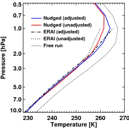
The vertical extent of the impact of the temperature adjustments is shown in Fig. 6, which shows profiles of global mean temperature averaged over the period between the temperature jumps in 1985 and 1998. Not surprisingly, the largest impact is at 1 hPa, where the adjusted run is about 2.5 K warmer than the unadjusted run. The difference changes sign at about 3 hPa, with the adjusted run being about 1 K colder at 4 hPa,
25
in accordance with the change in sign of the temperature adjustments at these levels (Fig. 4a). With the exception of the 1 hPa level for the adjusted run, the nudged runs are slightly warmer than their ERA-Interim counterparts (dashed and dotted curves). This is due to the fact that at all heights plotted here the free run is warmer than
ACPD
13, 25801–25825, 2013Removing discontinuities in
ERA-Interim temperatures
C. McLandress et al.
Title Page
Abstract Introduction
Conclusions References
Tables Figures
◭ ◮
◭ ◮
Back Close
Full Screen / Esc
Printer-friendly Version Interactive Discussion
Discussion
P
a
per
|
D
iscussion
P
a
per
|
Discussion
P
a
per
|
Discuss
ion
P
a
per
|
Interim, and the nudging pulls the model temperatures from their free running values towards the reanalysis.
The final two figures show the full seasonal cycle of temperature and ozone at 1 (Fig. 7) and 2 (Fig. 8) hPa. At 2 hPa the impact of including the adjustments is smaller than at 1 hPa, as expected based on Fig. 4a.
5
4 Summary
This technical note describes a simple procedure for removing unphysical temporal discontinuities in ERA-Interim global mean temperatures in the upper stratosphere in March 1985 and August 1998 for the purpose of improving chemistry-climate model simulations that are nudged to ERA-Interim winds and temperatures. The temperature
10
adjustments are derived from the global and monthly means at 1, 2, 3 and 5 hPa and are interpolated to a 6 h grid. Adjustments are not made to the post August 1998 data since they are treated as the absolute reference. We also note that our procedure cannot identify slow drifts that might exist within each of our analysis periods.
Two simulations using a version of the Canadian Middle Atmosphere Model that is
15
nudged to the three-dimensional 6 h ERA-Interim horizontal winds and temperatures are performed in order to assess the impact of including the temperature adjustments. The global mean temperatures in the upper stratosphere in the simulation without the adjustments exhibit the large temperature jumps found in ERA-Interim. Moreover, the ozone time series in this simulation also exhibit large discontinuities at the times of
20
the temperature jumps. This occurs because ozone is under photochemical control in the upper stratosphere. The inclusion of the adjusted nudging temperatures produces global mean temperatures and ozone that are devoid of the spurious jumps.
We encourage other modellers who are planning on performing nudged chemistry-climate model simulations to use the adjustment procedure described here. To
25
-ACPD
13, 25801–25825, 2013Removing discontinuities in
ERA-Interim temperatures
C. McLandress et al.
Title Page
Abstract Introduction
Conclusions References
Tables Figures
◭ ◮
◭ ◮
Back Close
Full Screen / Esc
Printer-friendly Version Interactive Discussion
Discussion
P
a
per
|
D
iscussion
P
a
per
|
Discussion
P
a
per
|
Discuss
ion
P
a
per
|
sets) from 1979 to 2010 at 1, 2, 3, and 5 hPa. These data can be found at http://www.cccma.ec.gc.ca/data/cmam/cmam30/era_interim_adjustment.
An important side issue arising from this work that is relevant to the REF-C1SD sim-ulations for CCMI is the initialization of simsim-ulations nudged to ERA-Interim from 1979 onwards. We have initialized ours using a spin-up nudged to ERA40. However, since
5
the tropical tropopause in ERA40 is warmer than in ERA-Interim, stratospheric wa-ter vapour in runs nudged to ERA40 is systematically higher than in runs nudged to ERA-Interim. This leads to a moist bias in the initial condition for the simulation nudged to ERA-interim, which takes about five years to disappear, consistent with the mean age of air in the upper stratosphere. During this adjustment period of decreasing water
10
vapour, there is an associated decrease in the destruction of ozone through HOx chem-istry, which outweighs ozone loss due to increasing concentrations of ozone-depleting substances and leads to an otherwise puzzling (and physically spurious) increase in upper stratospheric ozone during the first five years of the ERA-interim period. It is only after 1985 that upper stratospheric ozone starts to decline in the nudged simulation.
15
Thus, chemical constituents with a strong dependence on stratospheric water vapour (e.g. upper stratospheric ozone) should probably be disregarded from 1979 to about 1985 in simulations nudged to ERA-Interim unless the nudged climatology is identical to the spin-up climatology.
Acknowledgements. The authors are grateful to John Scinocca for numerous helpful
discus-20
sions and for comments on an earlier version of the manuscript, to Yanjun Jiao for performing the simulations, and to Adrian Simmons for a useful discussion that motivated this study as well as for comments on an earlier version of the manuscript. This work was funded by the Canadian Space Agency through the CMAM20 project.
ACPD
13, 25801–25825, 2013Removing discontinuities in
ERA-Interim temperatures
C. McLandress et al.
Title Page
Abstract Introduction
Conclusions References
Tables Figures
◭ ◮
◭ ◮
Back Close
Full Screen / Esc
Printer-friendly Version Interactive Discussion
Discussion
P
a
per
|
D
iscussion
P
a
per
|
Discussion
P
a
per
|
Discuss
ion
P
a
per
|
References
Dee, D., and Uppala, S.: Variational bias correction in ERA-Interim, ECMWF Technical Mem-orandum No. 575, European Centre for Medium-Range Weather Forecasts, Reading, UK, available at: http://www.ecmwf.int/publications/, 2008.
Dee, D. P., Uppala, S. M., Simmons, A. J., Berrisford, P., Poli, P., Kobayashi, S., Andrae, U.,
5
Balmaseda, M. A., Balsamo, G., Bauer, P., Bechtold, P., Beljaars, A. C. M., van de Berg, L., Bidlot, J., Bormann, N., Delsol, C., Dragani, R., Fuentes, M., Geer, A. J., Haimberger, L., Healy, S. B., Hersbach, H., Hólm, E. V., Isaksen, L., Kållberg, P., Köhler, M., Matricardi, M., McNally, A. P., Monge-Sanz, B. M., Morcrette, J.-J., Park, B.-K., Peubey, C., de Rosnay, P., Tavolato, C., Thépaut, J. N., and Vitart, F.: The ERA-Interim reanalysis: configuration and
10
performance of the data assimilation system, Q. J. Roy. Meteor. Soc., 137, 553–597, 2011. Eyring, V., Lamarque, J.-F., Hess, P., Arfeuille, F., Bowman, K., Chipperfield, M. P., Duncan, B.,
Fiore, A., Gettelman, A., Giorgetta, M. A., Granier, C., Hegglin, M., Kinnison, D., Kunze, M., Langematz, U., Luo, B., Martin, R., Matthes, K., Newman, P. A., Peter, T., Robock, A., Ry-erson, T., Saiz-Lopez, A., Salawitch, R., Schultz, M., Shepherd, T. G., Shindell, D.,
Staehe-15
lin, J., Tegtmeier, S., Thomason, L., Tilmes, S., Vernier, J.-P., Waugh, D. W., and Young, P. J.: Overview of IGAC/SPARC Chemistry-Climate Model Initiative (CCMI) community simulations in support of upcoming ozone and climate assessments, SPARC Newsletter, 40, 48–66, 2013.
Fomichev, V. I.: The radiative energy budget of the middle atmosphere and its parameterization
20
in general circulation models, J. Atmos. Sol.-Terr. Phys., 71, 1577–1585, 2009.
Kobayashi, S., Matricardi, M., Dee, D., and Uppala, S.: Toward a consistent reanalysis of the upper stratosphere based on radiance measurements from SSU and AMSU-A, Q. J. Roy. Meteor. Soc., 135, 2086–2099, 2009.
McLandress, C., Scinocca, J. F., Shepherd, T. G., Reader, M. C., and Manney, G. L.: Dynamical
25
control of the mesosphere by orographic and non-orographic gravity wave drag during the extended northern winters of 2006 and 2009, J. Atmos. Sci., 70, 2152–2161, 2013.
Rayner, N. A., Parker, D. E., Horton, E. B. Folland, C. K., Alexander, L. V., Rowell, D. P., Kent, E. C., and Kaplan, A.: Global analyses of sea surface temperature, sea ice, and night marine air temperature since the late nineteenth century, J. Geophys. Res., 108, 4407,
30
ACPD
13, 25801–25825, 2013Removing discontinuities in
ERA-Interim temperatures
C. McLandress et al.
Title Page
Abstract Introduction
Conclusions References
Tables Figures
◭ ◮
◭ ◮
Back Close
Full Screen / Esc
Printer-friendly Version Interactive Discussion
Discussion
P
a
per
|
D
iscussion
P
a
per
|
Discussion
P
a
per
|
Discuss
ion
P
a
per
|
Sato, M., Hansen, J. E., McCormick, M. P., and Pollack, J. B.: Stratospheric aerosol optical depths, 1850–1990, J. Geophys. Res., 98, 22987–22994, 1993.
Scinocca, J. F., McFarlane, N. A., Lazare, M., Li, J., and Plummer, D.: Technical Note: The CCCma third generation AGCM and its extension into the middle atmosphere, Atmos. Chem. Phys., 8, 7055–7074, doi:10.5194/acp-8-7055-2008, 2008.
5
Shepherd, T. G.: Stratosphere-troposphere coupling, J. Meteor. Soc. Japan, 80, 769–792, 2002.
SPARC CCMVal: SPARC Report on the evaluation of chemistry-climate models, edited by: Eyring, V., Shepherd, T. G., and Waugh, D. W., SPARC Report No. 5, WCRP-132, WMO/TD-No. 1526, 434 pp., available at: http://www.atmosp.physics.utoronto.ca/SPARC, 2010.
10
Uppala, S. M., Kållberg, P. W., Simmons, A. J., Andrae, U., da Costa Bechtold, V., Fior-ino, M., Gibson, J. K., Haseler, J., Hernandez, A., Kelly, G. A., Li, X., Onogi, K., Saari-nen, S., Sokka, N., Allan, R. P., Andersson, E., Arpe, K., Balmaseda, M. A., Bel-jaars, A. C. M., van de Berg, L., Bidlot, J., Bormann, N., Caires, S., Chevallier, F., Dethof, A., Dragosavac, M., Fisher, M., Fuentes, M., Hagemann, S., Hólm, E., Hoskins, B. J., Isaksen, L.,
15
Janssen, P. A. E. M., Jenne, R., McNally, A. P., Mahfouf, J.-F., Morcrette, J.-J., Rayner, N. A., Saunders, R. W., Simon, P., Sterl, A., Trenberth, K. E., Untch, A., Vasiljevic, D., Viterbo, P., and Woollen, J.: The ERA-40 re-analysis, Q. J. Roy. Meteor. Soc., 131, 2961–3012, 2005.
ACPD
13, 25801–25825, 2013Removing discontinuities in
ERA-Interim temperatures
C. McLandress et al.
Title Page
Abstract Introduction
Conclusions References
Tables Figures
◭ ◮
◭ ◮
Back Close
Full Screen / Esc
Printer-friendly Version Interactive Discussion
Discussion
P
a
per
|
D
iscussion
P
a
per
|
Discussion
P
a
per
|
Discuss
ion
P
a
per
|
Table 1.CoefficientsAml,n,Blm,nandCl,nused in Eq. (1) for generating the 6 hourly global mean temperature offsets using the first four harmonics of the annual cycle for the two time periods. Periodn=1 extends up to 12Z 21 March 1985; periodn=2 extends from 12Z 21 March 1985 to 00Z 1 August 1998. Units are K. In order to provide more precision, the coefficientsAml,nand Blm,nare multiplied by 10.
Period (n) Pressure (l) Cl,n Alm,n×10 Blm,n×10
ACPD
13, 25801–25825, 2013Removing discontinuities in
ERA-Interim temperatures
C. McLandress et al.
Title Page
Abstract Introduction
Conclusions References
Tables Figures
◭ ◮
◭ ◮
Back Close
Full Screen / Esc
Printer-friendly Version Interactive Discussion
Discussion
P
a
per
|
D
iscussion
P
a
per
|
Discussion
P
a
per
|
Discuss
ion
P
a
per
|
2
Fig. 1.Global and monthly mean ERA-Interim temperature anomalies at the top five pressure levels in the stratosphere. The curves at 2, 3, 5 and 7 hPa are shifted by 10 K with respect to the curve above. The “jump times” in March 1985 and August 1998 are denoted by the thin vertical lines. Tick marks on the horizontal axis denote January.
ACPD
13, 25801–25825, 2013Removing discontinuities in
ERA-Interim temperatures
C. McLandress et al.
Title Page
Abstract Introduction
Conclusions References
Tables Figures
◭ ◮
◭ ◮
Back Close
Full Screen / Esc
Printer-friendly Version Interactive Discussion
Discussion
P
a
per
|
D
iscussion
P
a
per
|
Discussion
P
a
per
|
Discuss
ion
P
a
per
|
Fig. 2.Global and monthly mean ERA-Interim temperatures at 1 hPa.(a)Unadjusted.(b)Deseasonalized (black) and fits to the deseasonalized time series computed over the three time periods using a linear trend and the F10.7 and volcanic aerosol time series (red). The red curves extend slightly beyond the ends of the data used for the fits to show the overlap region that is used to calculate the annual mean offsets, which are evaluated at the mid-point of the year the jump occurs denoted by the red crosses.(c)Deseasonalized time series with annual mean offsets included.
ACPD
13, 25801–25825, 2013Removing discontinuities in
ERA-Interim temperatures
C. McLandress et al.
Title Page
Abstract Introduction
Conclusions References
Tables Figures
◭ ◮
◭ ◮
Back Close
Full Screen / Esc
Printer-friendly Version Interactive Discussion
Discussion
P
a
per
|
D
iscussion
P
a
per
|
Discussion
P
a
per
|
Discuss
ion
P
a
per
|
1
Fig. 3. Global mean 6 hourly ERA-Interim temperatures at 1 hPa showing the jumps in (a)March 1985 and (b) August 1998: adjusted (blue) and unadjusted (red). The jump times (12Z 21 March 1985 and 00Z 1 August 1998) are denoted by the left pair of thin vertical lines. The second pair of vertical lines, which are ten days after the jump times, are shown in order to indicate the time scale of the transition after the jumps.
ACPD
13, 25801–25825, 2013Removing discontinuities in
ERA-Interim temperatures
C. McLandress et al.
Title Page
Abstract Introduction
Conclusions References
Tables Figures
◭ ◮
◭ ◮
Back Close
Full Screen / Esc
Printer-friendly Version Interactive Discussion
Discussion
P
a
per
|
D
iscussion
P
a
per
|
Discussion
P
a
per
|
Discuss
ion
P
a
per
|
2
Fig. 5.Global and monthly mean deseasonalized(a)temperature and(b)ozone volume mixing ratio at 1 hPa for the adjusted (blue) and unadjusted (red) nudged runs. The free run (i.e., unnudged) is shown in black solid; the old free run in black dotted; see text for details. After August 1998 the red curve underlies the blue since no adjustment is applied then.
ACPD
13, 25801–25825, 2013Removing discontinuities in
ERA-Interim temperatures
C. McLandress et al.
Title Page
Abstract Introduction
Conclusions References
Tables Figures
◭ ◮
◭ ◮
Back Close
Full Screen / Esc
Printer-friendly Version Interactive Discussion
Discussion
P
a
per
|
D
iscussion
P
a
per
|
Discussion
P
a
per
|
Discuss
ion
P
a
per
|
2
Fig. 7.Global and monthly mean(a)temperature and(b)ozone volume mixing ratio at 1 hPa for the adjusted (blue) and unadjusted (red) nudged runs. After August 1998 the red curve underlies the blue since no adjustment is applied then.
ACPD
13, 25801–25825, 2013Removing discontinuities in
ERA-Interim temperatures
C. McLandress et al.
Title Page
Abstract Introduction
Conclusions References
Tables Figures
◭ ◮
◭ ◮
Back Close
Full Screen / Esc
Printer-friendly Version Interactive Discussion
Discussion
P
a
per
|
D
iscussion
P
a
per
|
Discussion
P
a
per
|
Discuss
ion
P
a
per
|
2