Dynamic Programming applied to Medium Term
Hydrothermal Scheduling
Thais G. Siqueira and Marcelo G. Villalva
Abstract—The goal of this work is to present a better under-standing of the behavior of dynamic programming operating policies applied to the resolution of medium-term operational planning problem. Hydro plants located in different regions in Brazil will be considered for the analysis. The randomness of inflows will be treated and considered in the resolution of the problem using Dynamic Programming approaches. Then these results will be simulated from series of inflows.
Index Terms—hydro plants, hydrothermal scheduling, inflow uncertainty, dynamic programming, simulation
I. INTRODUCTION
The medium term hydrothermal scheduling (MTHS) prob-lem is quite complex due to some of its characteristics, specially the randomness of inflows. The MTHS aims to determine, for each stage (month) of the planning period (years), the amount of generation at each hydro and thermal plant which attends the load demand and minimizes the expected operation cost along the planning period.
Stochastic dynamic programming (SDP) has been the most suggested technique to solve the MTHS problem since it can adequately cope with the uncertainty of inflows and the nonlinear relations among variables. Although efficient in the treatment of river inflows as random variables described by probability distributions, the SDP technique is limited by the so-called ”curse of dimensionality” since its com-putational burden increases exponentially with the number of hydro plants. In order to overcome this difficulty one common solution adopted is to represent the hydro system by an aggregate model, as it is the case in the Brazilian power system. Alternatives to stochastic models for MTHS can be developed through operational policies based on deterministic models. The advantage of such approaches is their ability to handle multiple reservoir systems without the need of any modeling manipulation. Although some work has been done in the comparison between deterministic and stochastic approaches for MTHS, the discussion about the best approach to the problem is far from ending. The purpose of this paper is to present a discussion about different policies based on Dynamic Programming to solve MTHS. Hydro plants located in different regions of Brazil will be considered as case studies. The uncertainty of inflows will be modelled and the Box-Cox transformation will be used. One determinist model and three other stochastic models will be considered for solving the problem and finally these results will be simulated using inflows series. This paper is organized as follows: Section 1 presents the formulation of
Manuscript received July 30, 2016; revised August 8, 2016. This work was supported by Funcamp/Unicamp.
Prof. Thais G. Siqueira of Institute of Science and Technology, UNIFAL, Poc¸os de Caldas, Brasil, e-mail: [email protected]
Prof. Marcelo G. Villalva, School of Electrical and Computer Engineer-ing, UNICAMP, Campinas, Brasil, email: [email protected]
the MTHS problem, section 2 shows four different Dynamic Programming approaches that will be analysed in this paper. Section 3 reports the numerical results for the case studies and discusses the features and sensitivities of the different models. Section 4 summarizes the conclusions.
II. MTHSFORMULATION
The MTHS problem, in systems composed of a single hydro plant, considering the uncertainty of inflows, can be formulated as a nonlinear stochastic programming problem seeking the minimization of the expected operational cost and is given by:
min Ey
(
λt T−1
X
t=1
ψt(dt−pt)
)
+αT(xT) (1)
subject to:
xmedt =
xt+xt+1
2 (2)
pt=k[φ(xmedt )−θ(ut)−δ(qt)]qt, ∀ t (3) xt=xt−1+ (yt−qt)β, ∀t (4) ut=qt+st, ∀ t (5)
xt∈Xt (6)
vt∈Vt (7)
st≥0 (8)
x0 given (9)
In the above equations Ey: represents the expected value of the inflows ; T is the planning period;t is the index of the planning stages;λt: is a discount rate to convert cost for present; ψt(.) is the thermal cost function at stage t; gt is the thermal generation at stage t; dt is the energy demand at stage t; pt is the hydro generation at stage t, which is the product of a constant k, the water head given by the difference of forebay elevation φ(xt) and tailrace elevation
III. DYNAMICPROGRAMMINGMODELS FORMTHS For solving the problem (1)-(8) by SDP, the optimization problem is divided into stages and at each stage the optimal control variable is chosen in order to minimize the expected cost for each state of the system. The optimization process is based on a previous knowledge of the future possibilities and its consequences, satisfying the Bellman optimality principle, [2]. Thus the total operation cost from stage until the end of the planning period is obtained with the sum of the present cost at stage twith the optimal future cost of the following stages, which were previously determined. Since the problem is a stochastic one, the optimal control at each stage is obtained based on the probability distribution of the inflow at that stage, [3], [4], [7]. The dynamic programming recursive equation is given by:
Ft(xt) = min
qt,st
{ψt(dt−pt) +Ft+1(xt+1)} (10)
The recursive equation (10) is solved for each stagetsubject to equations (2) -(8).
The four policies based on dynamic programming models considered in this work will be detailed bellow.
A. Deterministic Dynamic Programming
In the Deterministic Dynamic Programming (DDP) the inflow for each monthmis known previously and calculated based on the historical values of each hydro plant. In this approach the long term average, ym, provides the inflow
arithmetical mean for each month for all N years of the historical.
ym= 1
N N
X
r=1
yr,m (11)
DDP can be considered as a particular case of SDP where the probability is assumed one if the inflow long term average for a certain month occurs.
The recursive equation for this particular case, where Qt
is the decision search space, can be written as:
αt−1(xt−1) =minqt∈Qt{ψt(dt−pt) +αt(xt)} (12)
where:
xt=xt−1+ (yt−qt)β (13)
B. Independent Stochastic Dynamic Programming
If one solves dynamic programming considering the in-flows monthly independent, the recursive equation will be similar to DDP and the only difference is the future cost that will be weighted by their probabilities pi considering the inflow discretization divided inN y parts.
Thus, the recursive equation of ISDP is given by:
αt−1(xt−1) =minqt∈Qt
N y
X
i=1
ψt(dt−pit) +αt(x i t) .pi
(14) where:
xit=xt−1+ (yit−qt)β (15)
and
pit=k[φ( xi
t+xt+1
2 )−θ(qt)−δ(qt)]qt (16)
C. Stochastic Dual Dynamic Programming
In the Stochastic Dual Dynamic Programming (SDDP) one supposes that in the beginning of each month the inflow that will occur is known. Each final month state is represented by a pair (stored volume at the end of the month; inflow of this month) [7]. The inflow distribution is represented by a inflow set and its probabilities. Each inflow is analysed separetely, resulting in different optimal individual decisions. For each combination of storage level and inflow, according to its discretization, an optimal decision is found. For a given storage level, each optimal decision takes to a total cost of operation. Thus, an expected cost is calculated with these different costs.
For this approach one considers the following recursive equation:
αt−1(xt−1) = N y
X
j=1
pjnminqt∈Qt[ψt(dt−p
j
t) +αt−1(xjt)]
o
(17)
xjt=xt−1+ (ytj−q j
t)β (18)
pjt =k[φ(
xjt+xt−1
2 )−θ(qt)−δ(qt)]qt (19)
D. Dependent Stochastic Dynamic Programming
When the inflows uncertainty is considered through a Markov chain, [6], leading to the dependent SDP (DSDP), the state variable changes to include the inflow of the previous stage, the probabilities are now calculated from the conditional probability density function and the recursive equation is modified to:
Ft(xt) = min
qt,st
{ψ(gt) +Eqt|qt−1{Ft+1(xt+1)}} (20)
Again, one solves the recursive equation (20) for each stage
taccording to equations (2)-(8).
In this work one represents the inflow uncertainty of the hydro plants by a Normal probability density function with Box-Cox transformation.
IV. CASESTUDIES
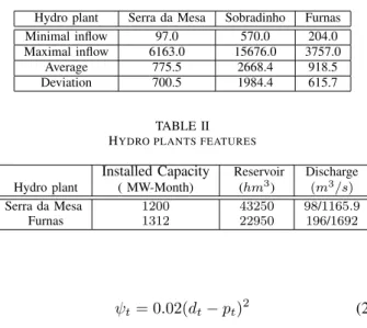
Two hydro plants were considered for the case studies: Serra da Mesa in the Tocantins River in northern region of Brazil, Furnas in the S˜ao Francisco River, located in the southeastern region of Brazil. In order to get equilibrated hydrothermal systems, the thermal plant capacity, in MW, was considered equal to the installed capacity of the hydro plants and the load demand was assumed constant.
TABLE I
STATISTICAL OF NATURAL INFLOWS OF HYDRO PLANTS.
Hydro plant Serra da Mesa Sobradinho Furnas Minimal inflow 97.0 570.0 204.0 Maximal inflow 6163.0 15676.0 3757.0
Average 775.5 2668.4 918.5 Deviation 700.5 1984.4 615.7
TABLE II HYDRO PLANTS FEATURES
Installed Capacity Reservoir Discharge Hydro plant ( MW-Month) (hm3)
(m3
/s) Serra da Mesa 1200 43250 98/1165.9
Furnas 1312 22950 196/1692
ψt= 0.02(dt−pt)2
(21)
The control policies were implemented and simulated in a monthly basis throughout the inflow historical sequence, which in this case begins in1931.
Table 1 shows some relevant statistical data of the hydro plants inflows. This information was used for modeling the inflow with the probability density function.
In the optimization process the planning period T con-sidered for the recursive equation solution was equal to120
with terminal cost null, αT(xT) = 0, ∀ xT.
For all DP policies, the discretization adopted for state variable was 100, and for the stochastic ones, the inflow variable was discretized into 10 possible values. A normal probability density function with Box-Cox transformation was adopted for modeling the inflows and the optimal param-eters were found by the likelihood test. The optimal values for Serra da Mesa and Furnas reservoir were λ∗ =−0.318
andλ∗=−0.539, respectively.
Cubic splines were used in the the interpolation of future costs.
Table 2 shows some operative data of the hydro plants selected for the case studies.
The forebay and tailrace elevations, φ(xt) and θ(qt), were calculated by 4th degree polynomial functions. The coefficient values of these polynomial function are shown in Table 3. These data will be used in the calculus of PD policies.
The DDP, ISDP, and DSDP were simulated through his-torical records since 1931and the NFN-SDP was simulated using an inflow forecast given by neural fuzzy network
TABLE III
FOREBAY AND TAILRACE ELEVATIONS POLYNOMIAL COEFFICIENTS OF HYDRO PLANTS
Coefficients Serra da Mesa Furnas φ(xt) a0 3.877328E+02 7.361261E+02
a1 3.487404E-03 3.193892E-03
a2 -8.567909E-08 -1.608703E-07
a3 1.233703E-12 5.076109E-12
a4 -7.135002E-18 -6.504317E-17
θ(qt) b0 3.327979E+02 6.716328E+02
b1 1.342970E-03 1.017380E-03
b2 8.819558E-08 -1.799719E-07
b3 -1.627669E-11 2.513280E-11
b4 0.000000E+00 0.000000E+00
TABLE IV
SERRA DAMESA SIMULATION RESULTS
Policy Generation (M W) Cost ($) Average Deviation Average AO 840.3 132.7 4135 DPP 815.7 177.9 4839.4 ISDP 818.1 165.3 4712.4 NFN-SDP 817.5 165.0 4724.3 DSDP 816.0 161.2 4726.5
TABLE V
FURNAS SIMULATION RESULTS
Policy Generation (MW) Cost ($) Average Deviation Average AO 727.8 148.3 7271.1 DDP 709.2 198.1 8029.0 ISDP 704.6 183.8 8037.7 NFN-SDP 707.9 209.2 8158.2 DSDP 708.1 192.9 8016.4
model. In this case, the forecast were based on neural networks and fuzzy logical [1]. An absolute optimal solution was considered as an upper bound for the operative policies analysed. This approach considers the total knowledge of the inflows.
Tables 4 and 5 show the simulation results for all policies investigated: the hydrothermal generation average and its deviation and the operation cost for Serra da Mesa and Furnas, respectively.
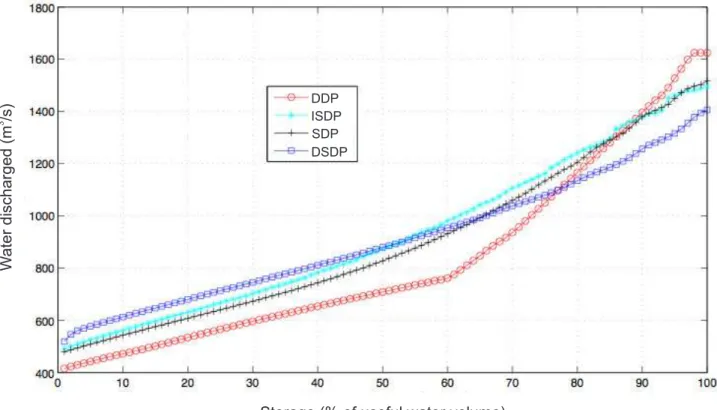
The discharged water trajectories for the DP policies: DDP (red), ISDP (green), SDP (black) and DSDP (blue) can be visualized in Figure 1 and Figure 3 for Serra da Mesa and Furnas hydro plants, respectively.
The behavior of stored volumes for the DP policies includ-ing the optimal absolute solution (full line in black): DDP (red), ISDP (blue), NFN-SDP (green) and DSDP (pink) can be visualized in Figure 2 and Figure 4 for Serra da Mesa and Furnas hydro plants, respectively.
According to the obtained simulation results for Serra da Mesa hydro plant the lower mean cost ($ 4712.4) was associted to ISDP policy. The higher mean generation, that was equal to818.1M W, was also provided by ISDP. DDP was the policy with worse performance, presenting the higher mean cost equal to $4839.4.
The difference between stochastical approaches, ISDP and DSDP, was equal to 0.29%. Analysing ISDP versus NFN-SDP there was a cost gain of 0.25% over INFN-SDP. Comparing DDP versus DSDP the difference was 2.3%. The perfor-mance difference between the best and worse policy was at about2.7%.
Thus, one concludes that due to the fact that DSDP explores the mensal correlation between the months of the year, there is no guarantee of this policy presents the best result.
The comparison of the obtained results for Serra da Mesa hydro plant are shown in Figure 1, that shows the discharged water, and Figure 2, that shows the stored water behavior for all policies investigated.
Storage (% of useful water volume)
W
ater discharged (m
/s)
3
ISDP SDP DSDP DDP
Fig. 1. Discharged water (m3
/s) of Serra da Mesa hydro plant for january.
Time (1935 - 1945)
Storage (% of useful water volume) ISDP
NFN-SDP DSDP
AO DDP
Storage (% of useful water volume)
W
ater discharged (m
/s)
3 ISDP
SDP DSDP DDP
Fig. 3. Discharged water (m3
/s) of Furnas hydro plant for january.
Time (1952 - 1961)
Storage (% of useful water volume)
ISDP NFN-SDP DSDP AO DDP
Fig. 4. Trajectory of stored volumes (%v.u.) of Furnas.
the average costs of DDP and DSDP, DDP generates1.1MW (0.15%) more, however, its average cost is 0.16% worse.
DDP presented higher average generation equal to 709.2 MW and this can be explained due to the fact that DDP has presented the higher spillaged water and took advantage of this water released that could be stored or spilled. The worse performance was associated to NFN-SDP policy with average cost equal to $ 8158.2.
V. CONCLUSION ANDREMARKS
Based on the simulation results it is possible to affirm that the policies performance were similar. The differences of average costs between the best and worse policy was nearly, 2.7% and 1.7% for Serra da Mesa and Furnas hydro plants, respectively.
Another conclusion is that the better performance not al-ways was associated to the most sophisticated inflow model. For instance, the better result for Serra da Mesa was given by ISDP that does not consider the inflow time correlation.
Another important conclusion of the numerical results was that DDP presented surprisingly a good performance, only 2.7%, and 0.15% worse that the better SDP policy for Serra da Mesa and Furnas, respectively.
The simulation results have shown that both deterministic approaches have provided quite similar performance, spe-cially regarding the operational cost.
REFERENCES
[1] Ballini R., Von Zuben F.J., ”Application of neural networks to adaptive control of nonlinear systems, Journal of IFAC, Volume 36 Issue 12,
December, 2000, Pages 1931-1933 .
[2] Bellman, R. E., 1957, ”Dynamic Programming”, Princeton University Press, Princeton, NJ.
[3] Bertsekas, D. P., 1976, ”Dynamic Programming and Stochastic Con-trol”, Academic Press.
[4] Bertsekas, D. P., 1987, ”Dynamic Programming: Deterministic and Stochastic Models”, Academic Press.
[5] Box, G. E. P., Jenkins, G. M., and Reinsel, G. C., 1994. ”Time Series Analysis, Forecasting and Control”, 3rd ed. Prentice Hall, Englewood Cliffs, NJ. Box, G., Cox D., 1964, ”An analysis of transformations”, J. R. Statistic Society, Serie B, 26, 211-252.
[6] Papoulis, A., 1921, ”Probability, random variables, and stochastic processes”, 4th edition, McGray-Hill, New York, NY.
[7] Stedinger, J. R., B. F. Sule, D. P. Loucks, ”Stochastic Dynamic Programming Models for Reservoir Operation Optimization”, Water Resources Research, 20(11), 1499-1505, 1984.
[8] Thyer, Mark, Kuczera, G., Wang, Q.J. (2002), ”Quantifying parameter uncertainty in stochastic models using the Box-Cox transformation”, J. Hydrol, 265, 246-257.