ISSN 1678-992X
ABSTRACT: The estimation of soil physical and chemical properties at non-sampled areas is valuable information for land management, sustainability and water yield. This work aimed to model and map soil physical-chemical properties by means of knowledge-based digital soil map-ping approach as a study case in two watersheds representative of different physiographical regions in Brazil. Two watersheds with contrasting soil-landscape features were studied regard-ing the spatial modelregard-ing and prediction of physical and chemical properties. Since the method uses only one value of soil property for each soil type, the way of choosing typical values as well the role of land use as a covariate in the prediction were tested. Mean prediction error (MPE) and root mean square prediction error (RMSPE) were used to assess the accuracy of the prediction methods. The knowledge-based digital soil mapping by means of fuzzy logics is an accurate option for spatial prediction of soil properties considering: 1) lesser intense sampling scheme; 2) scarce financial resources for intensive sampling in Brazil; 3) adequacy to properties with non-linearity distribution, such as saturated hydraulic conductivity. Land use seems to influence spatial distribution of soil properties thus, it was applied in the soil modeling and prediction. The way of choosing typical values for each condition varied not only according to the prediction method, but also with the nature of spatial distribution of each soil property.
Keywords: ANOVA test, spatial variability, fuzzy logic, typical values
Knowledge-based digital soil mapping for predicting soil properties in two
Michele Duarte de Menezes1*, Sérgio Henrique Godinho Silva1, Carlos Rogério de Mello2, Phillip Ray Owens3, Nilton Curi1
1Federal University of Lavras – Soil Science Dept., C.P. 3037 – 37200-000 – Lavras, MG – Brazil.
2Federal University of Lavras – Engineering Dept. 3Purdue University – Dept. of Agronomy, 915 W. State St. – 47906 – West Lafayette, IN – USA.
*Corresponding author <[email protected]>
Edited by: Silvia del Carmen Imhoff
Received March 15, 2016 Accepted February 01, 2017
Introduction
The estimation of soil physical and chemical prop-erties at non-sampled areas is valuable information for land management, sustainability and water yield. Differ-ent interpolation techniques have been used with varying degrees of success in order to create more accurate soil property maps (McBratney et al., 2003). From the pedo-metric approach, most techniques have high sampling density as the main driver for interpolation. In Brazil, where areas with intensive field observations are scarce, another quantitative procedure for spatial prediction should be considered. One approach with the advantage of low density of sampling (Shi et al., 2009) is the knowl-edge-based digital soil mapping technique, based on simi-larity vectors and parameters of fuzzy logic in an expert system (Zhu and Band, 1994; Zhu et al., 1997).
Similar to conventional soil survey, the knowledge of soil-landscape relationships is crucial for the accuracy of prediction of soil types and properties (Menezes et al., 2013), which is stablished and formalized by means of fuzzy membership curves (Shi et al., 2009). Spatially continuous soil property maps (Zhu et al., 1997), from only one representative value per soil type, can be gen-erated. Besides its low cost, it overcomes a conventional soil survey limitation, in which each soil-mapping unit assumes a unique value based on a soil profile described, which does not necessarily reflect the variability and continuous nature of soil properties within and between polygon mapping units (Menezes et al., 2014).
Two watersheds were chosen for this study, ac-cording to their representativeness in two different
representative watersheds
physiographical regions of Southern Minas Gerais: Man-tiqueira Range and Vertentes Fields physiographical re-gions. Both study sites are located in the Rio Grande watershed, which is an important water source for hy-droelectric energy production, where environmental is-sue is associated with the native forest that has been replaced by extensive pasture or crops with degraded lands (Viola et al., 2014; Beskow et al., 2013).
This work aimed to model and map soil physical and chemical properties from knowledge-based digital soil mapping, as a study case in two watersheds in con-trasting physiographical regions. The role of land use on organisms as a factor to form soils and their influence on predictions of soil physical and chemical properties was also tested. The way of choosing typical values to spatialize each condition and the role that land use plays as an environmental covariate were assessed into the spatial prediction.
Materials and Methods
Study sites
This study was conducted at Lavrinha Creek Wa-tershed (LCW) and Marcela Creek WaWa-tershed (MCW) located in the state of Minas Gerais, southeastern Brazil. Both watersheds are representative of the Rio Grande watershed, but they are located in different physio-graphical regions: Mantiqueira Range region (LCW) and Vertentes Fields region (MCW). LCW is located be-tween latitudes S 22º6’53” and 22º8’28” and longitudes W 44º26’21” and 44º28’39”, with area of 676 ha, with altitudes varying from 1,156 to 1,697. The average
an-Soils and Plant Nutrition
|
Resear
ch Ar
nual temperature is 15 °C and precipitation is 2,000 mm, with the native vegetation of the Atlantic Forest (Tropical Forest) and geology of gneiss. MCW is located between latitudes S 21º14’27” and 21º15’51” and longi-tudes W 44º30’58” and 44º29’29”, with area of 470 ha and altitudes varying from 958 m to 1,059. The average annual temperature is 19.7 °C and annual precipitation is 1.300 mm, with native vegetation of Cerrado (Brazil-ian savanna) and geology of mica schist. Both areas are located in Cwb domain, according to Koppen classifica-tion (Alvares et al., 2013), where the winter is cold and dry and summer is hot and humid.
Soil-landscape relationship
Considering the soil-landscape relationships at LCW, the alteration of gneiss resulted in predominance of Inceptisols (moderately developed and well-drained soils). The relief is steep with concave-convex hillsides and predominance of linear landforms and narrow floodplains. Endoaquents occupy the toeslope position, where the water table is near the surface in most part of the year (Menezes et al., 2014).
MCW has gentle undulated relief with extreme soil development. Oxisol is the most geographically expres-sive soil type, formed on stable and very old surfaces con-ductive to intense weathering-leaching under warm and moist climate, where organisms are very active (Motta et al., 2002). Inceptisols occupy the more dissected positions and more linear portions inside a convex macrolandform (Pelegrino et al., 2016). Endoaquents occupy the youngest surface on the toeslope (Silva et al., 2014).
Acrudox (hue 2.5YR or redder) occupies flatter and convex summit positions. Hapludox (hue 5YR) and Hapludox (hue 7.5YR or 10YR) occur from summit to footslope in the landscape. These colors show a preterit hydrological influence, where the type of orientation of parent material layers, by conditioning a different mois-ture regime in the two systems, exerted influence on the pedogenesis of the Acrudox and Hapludox. The hori-zontal orientation of the layers conditioned the genesis of Hapludox, with higher goethite/hematite ratio and consequently, yellowish colors, as the result of former soil moisture conditions that were different from that in redder soils. The inclined orientation of the layers conditioned, under similar topographic conditions, the formation of Acrudox, with better drainage and higher weathering-leaching intensity, higher hematite/goethite ratio and, consequently, reddish colors. Nowadays, due to the current climate conditions, both soils are well drained.
Soil property analyses
The physical and chemical properties analyzed were bulk density, by the volumetric ring method; soil organic matter, according to Walkley and Black (1934); drainable porosity, calculated by the difference between saturation moisture and soil moisture at field capacity; saturated hydraulic conductivity (Ksat) determined in
situ by constant flow permeameter; and total porosity, calculated according to the equation:
Total porosity bulk density particle density
% *
( )
= −
100 1
in which particle density was determined by the volu-metric flask method (Embrapa, 1997).
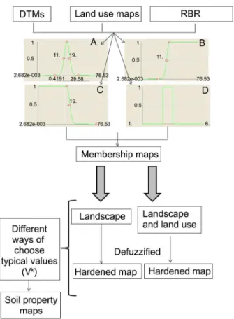
Knowledge-based digital soil mapping technique All steps accomplished since the creation of base maps until the soil property maps are presented in Figures 1A, B, C and D, which show the different function types or curve shapes. The knowledge on the soil-landscape relationships was qualitatively modeled using ArcSIE (Soil Inference Engine, version 9.2.402) (Shi et al., 2009). The Rule-Based Reasoning (RBR) in-ference method was used to define the relationship be-tween values of environmental variables (soil forming factors) and a given soil type. Considering the scale of variations of the studied sites, relief and organisms are the main drivers of soil variability, and the other soil forming factors are considered a constant. Additionally, terrain derivatives are strongly related to soil properties
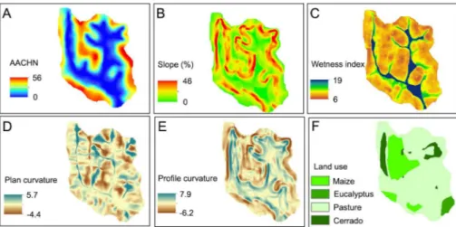
and have been useful in digital soil mapping for this rea-son (Akumu et al., 2015). Digital elevation models with pixels of 20 m resolution were generated from contour lines at 1:50,000 (IBGE) scale. DEM derivatives (digital terrain models – DTMs) (slope, altitude above the chan-nel network, plan curvature, profile curvature, and wet-ness index) were calculated using ArcGIS (ESRI, version 10) and SAGA GIS (System for Automated Geoscientific Analysis, version 2.1.0). DTMs have been frequently used as a proxy of current relief conditions (Heuvelink and Webster, 2001). DEM and DTMs, as well as land use raster maps, are presented in Figure 2 (A – altitude, B – slope, C – wetness index, D – plan curvature, E – profile curvature and F – land use) and Figure 3 (A – altitude above the channel network, B – slope, C – wet-ness index, D – plan curvature, E – profile curvature and F – land use). DTMs and ranges associated with each soil type in the maps were used to define membership or optimality functions (curves), which, in turn, define
the relationship between the values of an environmen-tal feature and soil type. The curve shapes bell, S, and Z were used for soil-landscape modelling, presented in Figures 1A, B, and C respectively. The Y axis shows the optimality value varying from 0 to 1, and the X axis the variation of DTMs values. The initial output from the in-ference process is a series of fuzzy membership maps in raster format, one for each soil type under consideration (Shi et al., 2009), representing similarities of each pixel in the landscape to the soil types. From those maps, the spatially continuous soil property maps derived from similarity vectors are generated, according to the for-mula (Zhu et al., 1997):
V S V
S
ij k n
ij k k
k n
ij k
= =
=
∑
∑
*
1
1
where Vij is the estimated physical or chemical prop-erty at location (i,j), Vk is a typical value of soil type k
Figure 2 – Digital terrain models and land use map of Lavrinha Creek Watershed. A) digital elevation model; B) slope; C) wetness index; D) plan curvature; E) profile curvature; F) land use.
(e.g. Udepts1), and n is the total number of prescribed soil types for the area. The typical value consists of the central concept of soil property value for each soil type, which is generally obtained at a soil profile in a polygon from conventional soil survey.
Different land uses were considered in the predic-tion, since they represent organisms as a soil-forming factor, which in turn, can influence the soil physical and chemical properties distribution. In order to assess whether soil properties are significantly influenced by different land uses, analyses of variance (ANOVA) were made by the F test (p < 0.01 or p < 0.05). Land uses at LCW are native forest (Atlantic Forest), natural regen-eration forest, pasture and wetland (Figure 2F), while land uses at MCW are Cerrado (Brazilian savanna), pas-ture, maize and eucalyptus crops (Figure 3F). The box-cox procedure was carried out to determine the suit-able type of transformation for ANOVA. Ksat was log transformed. The statistical analyses were performed in SAS (Statistical Analysis System Institute, version 9.2). If ANOVA test pointed out the influence of land use, in such cases, the typical value Vk came from the
com-bination of soil (modelled using S-, Z-, and bell-shaped optimality curves) and land use k to form soil type, e.g. Udepts1 under pasture. In ArcSIE, land use raster map was used as categorical data (data do not have quantita-tive meaning, values are only for labeling or categorizing different land uses) and overlaid with all soil types, us-ing the function type Nominal (Shi et al., 2009), and the shape of the optimality curve is presented in Figure 1D. The maximum fuzzy membership value specified for each land use is 1. Since there are four different types of land uses at each watershed, the maps were reclassified in integer values that represent land use types.
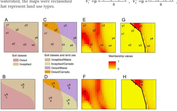
In this study, except for organic matter, most of the studied soil properties (bulk density, total porosity, drainable porosity, and hydraulic saturated conductiv-ity) are not frequently analyzed in soil profiles of soil surveys. Thus, the sampling scheme started from a dense grid design, but only a few points were used in the prediction in which different ways of choosing rep-resentative values for spatial prediction were tested. The sampling scheme is a current discussion in digital soil mapping community, since it is one of the main driv-ers of costs and prediction accuracy (Silva et al., 2015). The full data set comprehend the pre-defined topsoil sampling (0-15 cm) at both watersheds. A total of 198 points were sampled at LCW, following the 300 × 300 m regular grids as well as a refined scale of 60 × 60 m and 20 × 20 m, and two transects with the distance of 20 m between points (comprising 54 and 14 sampled points per transect). A total of 165 points were sampled at MCW, following the 240 × 240 m regular grids and a refined scale of 60 × 60 m. This sampling scheme with high density was required to test the way of choosing typical values in this study. Figures 4A, B, C, D, E, F, G and H show the different ways of choosing typical val-ues tested according to the sampled points, as follows: a) mean soil property value into each polygon of a soil type from the hardened map (Figures 4A and B). The data set for prediction was plotted into the soil type hardened map, the mean value was calculated for each soil type, and then used as Vk. In this study, we called this method
generically as mean. In Figure 4A, the example of mean value shows the hardened or defuzzified map,
Vk x x x x
1 1 2 3 4
4
=µ= + + +
,
Vk y y y y2
1 2 3 4
4
=µ= + + +
,
where xn and yn are sampled soil property values, whose mean within the polygon was used as Vk; b) mean soil
property value in each polygon that results from the soil type hardened map overlaid on land use raster map, if the ANOVA test shows that land use influences soil properties (Figures 4C and D). It was generically re-ferred to in this study as mean and the land use method in comparison with the mean method aforementioned, this one promotes more stratification and more typical values were used to generate prediction soil property maps. Thus, according to Figure 4B,
Vk y y
3 1 2
2
=µ= + ,
Vk x x Vk y y
4
1 2
5
3 4
2 2
=µ= + , =µ= +
,
Vk x x6
3 4
2
=µ= +
c) point geographically located on the pixel with high-est membership value for the correspondent soil type, referred to in this study as the landscape method (Fig-ures 4E and F). The fuzzy membership value for a given soil type shows that Vk x
7 = 1, since this sampled point is
located at the pixel with the highest membership among all points; d) point geographically located on the pixel with highest membership value for the correspondent soil type, but overlaid on land use raster map, if the ANOVA test showed that land use influenced soil prop-erties (Figures 4G and H). It was referred to in this study as landscape and land use method. Thus, membership maps were obtained from the soil-landscape modelling, but is this case, land use was also considered for each soil type, as showed by the black line in Figures 4G and H. The typical value in this case Vk y
8 = 3: the highest
membership value among all sampled points.
Comparison of methods
In order to create one independent validation data set to evaluate the performance of prediction methods, the total data set was divided into interpolation and vali-dation sets. Of the total number of places sampled, 25 points were used for validation at LCW and 20 points at MCW, both randomly chosen. The validation data set was not used in the models to develop predictions. Two indices were calculated from the observed and predicted values: the mean prediction error (MPE) and the root mean square prediction error (RMSPE). The MPE was calculated by comparing estimated values ( ( ))z s j with
the validation points ( ( ))z sj
∗ of Ksat:
MPE
l j z s z s l j j =
( )
−( )
=∑
1 1 ˆ *and the root mean square prediction error (RMSPE):
RMSPE
l j z s z s l j j =
( )
−( )
=∑
1 1 2 ˆ *where l is the number of validation points. The MPE measures the bias of prediction, and the RMSPE mea-sures the prediction accuracy.
Results and Discussion
The descriptive statistics of full, interpolation and validation data set (mean, media, skewness, coefficient of variation, minimum and maximum) of soil proper-ties can be viewed at Menezes et al. (2016). Validation and interpolation data sets showed quite similar sta-tistical characteristics. Among the soil properties, Ksat showed higher coefficient of variation and skewness. Skewness quantifies how symmetrical the distribution is in which values far from zero indicate long tails (left or right) and asymmetrical distribution. Thus, Ksat has non-normal distribution at both watersheds (Menezes et al., 2016).
Knowledge formalization by means of optimality curves
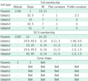
The soil-landscape relationship above described in the Materials and Methods section were quantified and formalized by a set of rules that relates to raster maps. The processes of knowledge formalization in ArcSIE Rule-Based Reasoning method means the establishment of optimality or membership curves, setting the param-eters to build S-, Z-, and bell-shaped curves. Threshold values related with DTMs were identified and assigned to each soil-mapping unit, according to soil scientists’ knowledge, and to a soil map from previous soil sur-vey (Menezes et al., 2014). It is the basis for establishing the membership maps for each soil type. Details on the shape of optimality curves as well as the parameters to stablish them from DTMs are presented in the Table 1.
At LCW, higher values of WI and lower values of slope were used to map Fluvents in flat alluvial areas (footslope). Inceptisols occupy the well-drained portions
Table 1 –Ranges of optimality curves of soil types at Lavrinha Creek Watershed.
Soil type1 Full membership
Altitude Slope WI Plan curvature Profile curvature
Fluvents 1156 1 15; 21 -
-Udepts1 - 32; 5 7 1 2.3
Udepts2 - 15 7 -1 0
Udepts3 - 32; 5 7 -1 0
Udepts4 - 51 7 -1 0
50 % membership
Fluvents 1200 10 14; 22 -
-Udepts1 - 19.5; 45.5 0; 14 0.11; 3 1.56; 9.5 Udepts2 - 10; 20 0; 14 -11; 0 -1.5; 1.5 Udepts3 - 19.5; 45.5 0; 14 -11; 0 -1.5; 1.5 Udepts4 - 45; 95 0; 14 -11; 0 -1.5; 1.5
Curve shape
Fluvents Z Z Bell -
-Udepts1 - Bell Bell Bell Bell
Udepts2 - Bell Bell Bell Bell
Udepts3 - Bell Bell Bell Bell
Udepts4 - Bell Bell Bell Bell
of the landscape with lower values of WI (wetness in-dex) (summit, shoulder, and backslope) formed by dif-ferent combinations and ranges of slope, plan and pro-file curvatures.
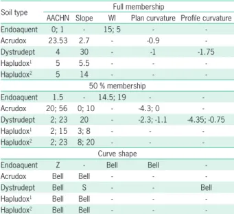
In MCW, Acrudox usually occupies flat summit positions in a more convex landform, expressed by higher values of Altitude Above the Channel Network (AACHN), lower values of slope and negative values of plan curvature. AACHN describes the vertical distance between each cell of a raster grid and the elevation of the nearest drainage channel cell connected with the respective grid cell of a DEM. The Hapludox is pres-ent on shoulder, backslope, and footslope positions (in-termediate values of AACHN and gentle slopes). Two instances were applied to Inceptisols: one considering steeper slopes, and another for plan and profile curva-tures. Two instances were necessary in order to formal-ize the knowledge on Inceptisols in this watershed: they occupy the more dissected positions and more linear portions inside a convex macrolandform. ArcSIE shows a general inference equation that allows integrating optimality values and then, the optimality values are generated for the whole instance, based on individual features (Shi, 2013). In this case, this integration is nec-essary through the multiplication function, since there are two different soil-landscape relationships for the Inceptisol instance. Endoaquents are located in lower AACHN and higher WI values. The ranges of DTMs are presented in Table 2. These instances are only related to terrain and soil types and have been frequently used to map soil properties (Brown et al., 2012; Adhikari et al., 2013; Vaysse and Lagacherie, 2015). Thus, whether land use maps could improve the accuracy of mapping is further discussed.
ANOVA test
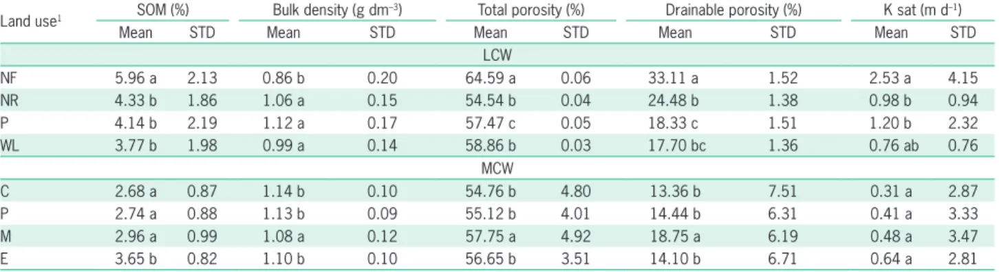
The ANOVA test was used to support the de-cision to apply land use as categorical information to map soil property. In other words, the test was run to verify whether there were differences between the dif-ferent types of land use (categorical map) according to soil physical properties. Abrupt changes in boundaries provided valuable categorical information to interpret soil property variation, and the variation between and within polygons are frequently assessed by the ANO-VA test (Oberthür et al., 1996; Liu et al., 2006; Molin and Castro, 2008). Except for Ksat in MCW, the vari-ance between land uses was statistically significant in both watersheds, meaning that land use affected physi-cal properties. Soils in MCW are mainly Oxisols, whose structure helps to explain the pattern variability. The adequate physical properties of Oxisols for soil manage-ment and intensive uses are mainly influenced by their high aggregate stability (Ajayi et al., 2009). For other soil properties, not only was the soil type modelling consid-ered, but also land use as a categorical optimality curve. Summary statistics of soil physical properties for the data stratified into four land uses are listed in Table 3. These results guided the way of using maps of land use in ArcSIE in which different types of land use were joined or treated separately, based on the mean test for separation. For example, the soil organic matter mean test in LCW showed that native vegetation is statistical-ly different from other land uses. Thus, the raster map was reclassified into two different nominal categories for each soil type with crisp boundaries: one nominal value for native vegetation and another nominal value for natural regeneration, pasture and wetland. Thus, a soil unit was created by the combination of soil type and land use. However, the issue here is whether the cat-egorical maps of land use can indeed improve accuracy to predict physical properties.
Assessment of prediction methods
Table 4 presents the statistical accuracy indexes for predictions, considering different ways to choose typical values at LCW and MCW. For each of soil prop-erty, a method with suitable accuracy was found, with MPE and RMSPE closer to zero. However, making com-parisons within same soil property, the methods per-formed in contrast, with extreme high values of MPE and RMSPE in some cases. Considering results from the literature related with soil physical properties, most results showed suitable accuracy indexes, similar to those presented in this work, but they are mostly related to soil texture mapping (Akumu et al., 2015; Qi et al., 2006; Zhu et al., 2010). Thus, it is not possible to make any specific comparison between MPE and RM-SPE values.
The use of similarity vectors and fuzzy logics for mapping soil texture in a work developed by Ashtekar et al. (2014) resulted in model and validation sets rath-er biased, and failed to capture the spatial variability Table 2 –Ranges of optimality curves of soil types at Marcela Creek
Watershed.
Soil type Full membership
AACHN Slope WI Plan curvature Profile curvature
Endoaquent 0; 1 - 15; 5 -
-Acrudox 23.53 2.7 - -0.9
-Dystrudept 4 30 - -1 -1.75
Hapludox1 5 5.5 - -
-Hapludox2 5 14 - -
-50 % membership
Endoaquent 1.5 - 14.5; 19 -
-Acrudox 20; 56 0; 10 - -4.3; 0 -Dystrudept 2; 23 20 - -2.3; -1.1 -4.35; -0.75
Hapludox1 2; 15 3; 8 - -
-Hapludox2 2; 23 8; 20 - -
-Curve shape
Endoaquent Z - Bell Bell
-Acrudox Bell Bell - -
-Dystrudept Bell S - - Bell
Hapludox1 Bell Bell - -
-Hapludox2 Bell Bell - -
of properties. Such results highlight the importance of choosing a representative data set, contrary to this case in which sampling was constrained to places nearby roads due to the access limitation throughout the study site. A weighted average of the fuzzy membership val-ues and the typical soil property valval-ues of the soil types is done pixel by pixel. This fact highlights the impor-tance of choosing sampling places that represent the central and representative value of the soil type, in or-der to avoid the pixel population of each instance with unreal values. The representative values obtained from a mean value of sampled point data outlying prop-erty values may cause over (positive MPE) or under (negative MPE) estimation of predicted soil properties (Ashtekar et al., 2014).
Fuzzy membership maps represent the uncer-tainty of prediction. The higher the value, the closer the central concept used for modeling soil type in the landscape. In this sense, if knowledge-based method postulates that a representative value should be cho-sen, membership maps have a potential for guiding sampling in the field campaign. For that, deep knowl-edge of the area is necessary to create accurate models and consequently membership maps.
Not only the way of choosing typical values should be considered to compare accuracy of predic-tions, but also the variation nature of each soil
prop-erty. Bulk density showed low coefficient of variation and lower values of RMSPE and MPE at both water-sheds (Menezes et al., 2016). In this case, the lesser variation might result in better agreement between dicted and observed (validation) values for all the pre-diction methods tested. The opposite trend was found for drainable porosity.
LCW shows a general trend that maps of land use applied to modelling promoted better accuracy. This could be related with the number of points used in the modelling, which are higher in models that use soil type and land use information, improving representa-tiveness of spatial variability. In this case, one typical value is required for each combination of soil type and land use, whose number of combinations is dictated by ANOVA, whereas those models developed only consid-ering soil types, required only 5 points for the spatial prediction (one typical value per each soil type). The types of land use are very contrasting when compar-ing pasture to tropical Atlantic Forest, which has a dense canopy and higher soil organic matter content. At MCW, where the relief is gentle with predominance of Oxisols under pasture, the prediction accuracy is overall better in which the use of mean typical values showed some of the best accurate predictions.
Ksat values at LCW and MCW (Menezes et al., 2016), as well as in other studies (Moustafa, 2000), Table 3 – Statistics of soil properties at Lavrinha Creek Watershed (LCW) and Marcela Creek Watershed (MCW).
Land use1 SOM (%) Bulk density (g dm
–3) Total porosity (%) Drainable porosity (%) K sat (m d–1)
Mean STD Mean STD Mean STD Mean STD Mean STD
LCW
NF 5.96 a 2.13 0.86 b 0.20 64.59 a 0.06 33.11 a 1.52 2.53 a 4.15
NR 4.33 b 1.86 1.06 a 0.15 54.54 b 0.04 24.48 b 1.38 0.98 b 0.94
P 4.14 b 2.19 1.12 a 0.17 57.47 c 0.05 18.33 c 1.51 1.20 b 2.32
WL 3.77 b 1.98 0.99 a 0.14 58.86 b 0.03 17.70 bc 1.36 0.76 ab 0.76
MCW
C 2.68 a 0.87 1.14 b 0.10 54.76 b 4.80 13.36 b 7.51 0.31 a 2.87
P 2.74 a 0.88 1.13 b 0.09 55.12 b 4.01 14.44 b 6.31 0.41 a 3.33
M 2.96 a 0.99 1.08 a 0.12 57.75 a 4.92 18.75 a 6.19 0.48 a 3.47
E 3.65 b 0.82 1.10 b 0.10 56.65 b 3.51 14.10 b 6.71 0.64 a 2.81
1Land use: NF = native forest; NR = natural regeneration; P = pasture; WL = wetland; M = maize; C = Cerrado; E = eucalyptus; STD = standard deviation; SOM = soil organic matter; Ksat = saturated hydraulic conductivity. Means followed by the same letter do not differ significantly (p < 0.05) within columns.
Table 4 – Comparison of interpolation methods at Lavrinha Creek Watershed (LCW) and Marcela Creek Watershed (MCW).
SOM Bulk density Total porosity Drainable porosity Ksat SOM Bulk density Total porosity Drainable porosity Ksat
LCW MCW
Mean MPE -2.00 -0.11 1.87 1.61 0.39 0.63 0.00 0.50 0.54 -0.01
RMSPE 10.01 0.56 9.34 8.05 1.93 2.80 0.01 2.24 2.43 0.06
Mean and land use MPE -1.95 0.02 1.07 2.40 0.39 0.53 -0.02 0.46 1.26
-RMSPE 9.75 0.12 5.35 12.01 1.93 2.38 0.08 2.02 5.62
-Landscape MPE -1.81 0.13 -1.81 -5.84 0.26 0.28 -0.01 0.45 -3.59 0.44
RMSPE 9.04 0.62 9.07 29.17 1.28 1.24 0.02 2.06 16.07 1.88
Landscape and land use MPE -1.11 0.06 -1.55 -0.40 0.30 0.14 -0.02 0.66 -1.35
-RMSPE 5.57 0.29 7.75 1.99 1.15 0.65 0.07 2.94 6.03
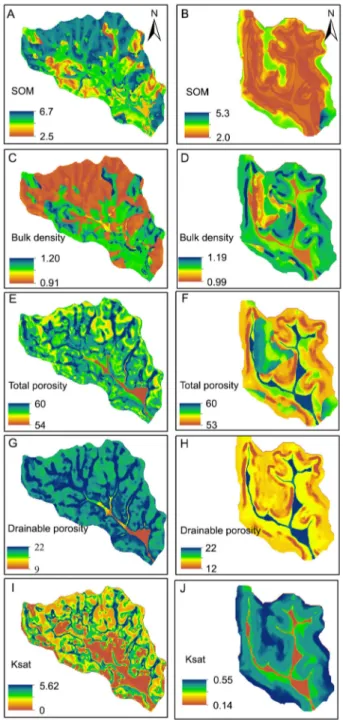
Figure 5 – The best prediction maps of soil physical and chemical properties. SOM = soil organic matter; Ksat = saturated hydraulic conductivity; A) landscape and land use used for SOM, C) mean and land use for bulk density, E) mean and land use for total porosity, G) landscape and land use for drainable porosity, and I) landscape for Ksat prediction at Lavrinha Creek Watershed; B) landscape and land use for SOM, D) mean for bulk density , F) mean and land use for total porosity, H) mean for drainable porosity, J) mean for Ksat at Marcela Creek Watershed.
have been recognized for their high spatial variability, skewed frequency and non-normality of distribution. Data normality can influence the estimation of certain spatial interpolation methods that assume input data are normally distributed around the mean (Li and Heap, 2011), e.g., kriging or linear regression. In these cases, data transformation is required and back-transformation brings back the predictions to the original scale. How-ever, back-transforming the estimated values can be problematic because exponentiation tends to exaggerate any interpolation-related error (Goovaerts, 1999). In this study, as already pointed out by Zhu et al. (2010), simi-larity vectors have an inherent non-linearity and can be used to describe and model non-linear variation of Ksat, overcoming the limitation of some interpolation meth-ods. The MPE and RMSPE values closer to zero show high accuracy of the presented method to map Ksat in both watersheds.
Prediction maps
The best prediction maps of each soil property are presented in Figures 5A, B, C, D, E, F, G, H, I and J. Figures 5A, C, E, G, and I show respectively landscape and land use used in prediction of soil organic matter, mean and land use for bulk density and total porosity, landscape and land use for drainable porosity predic-tion and landscape for Ksat predicpredic-tion at LCW. Figures 5B, D, F, H, and J show respectively landscape and land use for soil organic matter prediction, mean for bulk density, mean and land use for total porosity, and mean for drainable porosity and Ksat at MCW.
Since the knowledge-based technique incorpored the pedologist knowledge into the modelling, it is pos-sible to observe the continous nature of spatial distri-bution in each soil type (Tables 1 and 2) and/or land use (when it was used in the prediction), providing a real-istic portrayal of variation without a smoothing effect. This continuous variation is an advantage to capture spatial prediction, since soil property maps generated from conventional soil survey maps (polygon-based) are not sufficient due to general low level of detail (Zhu et al., 2010; Menezes et al., 2014).
There is a tendency for predicted soil property values to be stratified by soil type, especially those where a polygon raster map is used. In some cases, this artefact of polygon in spatial prediction is clear, as in Figure 5A, due to the use of polygon of eucalyptus land use (Figure 3F). Because knowledge-based digital soil mapping technique uses only one typical value per soil type for spatial prediction, the range of predicted properties are rather different from the interpolation data set range (Menezes et al., 2016), which can com-promise prediction accuracy.
At LCW, the relief seems to influence the veg-etation cover indirectly, since pasture is preferably implanted in flatter and lower areas. In addition, the higher soil organic matter content detected at higher altitudes (Figure 2A) was probably due to lower
or-ganic matter (Gessler et al., 2000), which, in turn, may explain the lower bulk density, higher total porosity, higher drainable porosity and Ksat in the same portions of the landscape, where the land use is native forest or natural regeneration (Figure 2F). The opposite situation happens in pasture areas.
At MCW, the soil organic matter prediction might be influenced by land use, revealing higher values in Cerrado and eucalyptus areas in the eastern side of the watershed (Figure 3F). Lower values of soil organic matter were found under pasture areas, which is the predominant land use in this watershed. Water distri-bution in landscapes stricly controls soil carbon dynam-ics (Gessler et al., 2000), even though the floodplain did not show higher values of soil organic matter, which may be due to the very high vertical and lateral spatial variability of characteristics, typical of these lowland environments. Soil organic matter maps showed higher values in the convex summit. Gessler et al. (2000) high-light the combination of higher weathering-leaching, very low natural fertility, low temperatures in the past, and limited activity of microorganisms might have con-tributed for the organic matter accumulation in this landscape position.
Differently from the other physical properties studied, the Ksat values are also influenced by soil properties at depth. Therefore, the spatial variability of this soil property may be related to properties better expressed in the B horizon of soils. Higher values of Ksat were found in Oxisols, where the adequate physi-cal properties are mainly influenced by aggregate sta-bility, as mentioned before. This trend was not followed by the total porosity and drainable porosity (topsoil). In the topsoil, even for Oxisols, the frequent wetting and drying cycles could be responsible for the decrease in aggregate stability (Caron et al., 1992), where the granular structure behaves as a blocky structure (Ajayi et al., 2009). Lower values of bulk density and higher values of total porosity were found in areas with rela-tively higher values of soil organic matter, as well as in the Cerrado area. Total porosity seems to be related with land use as well, as observed in areas under maize crops.
Conclusions
The knowledge-based digital soil mapping is an accurate option for spatial prediction of soil properties considering: 1) a less intense sampling scheme; and 2) scarce resources for high density samplings in Brazil; 3) adequacy to properties with non-linearity distribution, as Ksat.
Land use influences the spatial distribution of soil properties thus it was applied in the soil modelling and prediction. The way of choosing typical values varied not only according to the prediction method, but also with the nature of spatial distribution of each soil prop-erty.
References
Adhikari, K.; Kheir, R.B.; Greve, M.B.; Bocher, P.K.; Malone, B.P.; Minasny, B.; McBratney, A.B.; Greve, M.H. 2013. High-resolution 3-D mapping of soil texture in Denmark. Soil Science Society of America Journal 77: 860-876.
Ajayi, A.E.; Dias Junior, M.S.; Curi, N.; Gontijo, I.; Araujo-Junior, C.F.; Vasconcelos Júnior, A.I. 2009. Relation of strength and mineralogical attributes in Brazilian Latosols. Soil and Tillage Research 102: 14-18.
Akumu, C.E.; Johnson, J.A.; Etheridge, D.; Uhlig, P.; Woods, M.; Pitt, D.G.; McMurray, S. 2015. GIS-fuzzy logic based approach in modeling soil texture: using parts of the Clay Belt and Hornepayne region in Ontario Canada as a case study. Geoderma 239: 13-24.
Alvares, C.A.; Stape, J.L; Sentelhas P.C.; Gonçalves, J.L.M.; Sparovek, G. 2013. Köppen's climate classification map for Brazil. Meteorologische Zeitschrift. 22: 711-728.
Angers, D.A.; Bolinder, M.A.; Carter, M.R.; Gregorich, E.G.; Drury, C.F.; Liang, B.C.; Voroney, R.P.; Simard, R.R.; Donald, R.G.; Beyaert, R.P.; Martel, J. 1997. Impact of tillage practices on organic carbon and nitrogen storage in cool humid soils of eastern Canada. Soil and Tillage Research 41: 191-201. Ashtekar, J.M.; Owens, P.R.; Brown, R.A.; Winzeler, H.E.;
Dorantes, M.; Libohova, Z.; Silva, M.A.; Castro, A. 2014. Digital mapping of soil properties and associated uncertainties in the Llanos Orientales, South America. p. 367-373. In: Arrouays, D.; McKenzie, N.; Hempl, J.; Forges, A.C.R.; McBratney, A.B., eds. GlobalSoilMap: basis of the global spatial information system. CRC Press, Boca Raton, FL, USA.
Beskow, S.; Norton, L.D.; Mello, C.R. 2013. Hydrological prediction in a tropical watershed dominated by Oxisols using a distributed hydrological model. Water Resources Management 27: 341-363.
Brown, R.A.; McDaniel, P.; Gessler, P.E. 2012. Terrain attribute modeling of volcanic ash distributions in northern Idaho. Soil Science Society of America Journal 76: 179-187.
Caron, J.; Kay, B.D.; Stone, J.A. 1992. Improvement of structural stability of clay loam with drying. Soil Science Society of America Journal 56: 1583-1590.
Empresa Brasileira de Pesquisa Agropecuária [EMBRAPA]. 1997. Manual of Soil Analysis Method = Manual de Métodos de Análise do Solo. Centro Nacional de Pesquisa de Solos. EMBRAPRA-CNPS, Rio de Janeiro, RJ, Brazil (in Portuguese). Gessler, P.E.; Chadwick, O.A.; Chamran, F.; Althouse, L.; Holmes,
K. 2000. Modeling soil-landscape and ecosystem properties using terrain attributes. Soil Science Society of America Journal 64: 2046-2056.
Goovaerts, P. 1999. Geostatistics in soil science: state-of-the-art and perspectives. Geoderma 89: 1-45.
Heuvelink, G.B.M.; Webster, R. 2001. Modelling soil variation: past, present, and future. Geoderma 100: 269-301.
Li, J.; Heap, A.D. 2011. A review of comparative studies of spatial interpolation methods in environmental sciences: performance and impact factors. Ecological Informatics 6: 228-241. Liu, T.L.; Juang, K.W.; Lee, D.Y. 2006. Interpolating soil properties
McBratney, A.B.; Santos, M.L.M.; Minasny, B. 2003. On digital soil mapping. Geoderma 117: 3-52.
Menezes, M.D.; Silva, S.H.G.; Mello, C.R.; Owens, P.R.; Curi, N. 2014. Solum depth spatial prediction comparing conventional with knowledge-based digital soil mapping. Scientia Agricola 71: 316-323.
Menezes, M.D.; Silva, S.H.G.; Mello, C.R.; Owens, P.R.; Curi, N. 2016. Spatial prediction of soil properties in two contrasting physiographic regions in Brazil. Scientia Agricola 73: 274-285. Menezes, M.D.; Silva, S.H.G.; Owens, P.R.; Curi, N. 2013.
Digital soil mapping approach based on fuzzy logic and expert knowledge. Ciência e Agrotecnologia 37: 287-298.
Molin, J.P.; Castro, C.N. 2008. Establishing management zones using soil electrical conductivity and other soil properties by the fuzzy clustering technique. Scientia Agrícola 65: 567-573. Motta, P.E.F.; Curi, N.; Franzmeier, D.P. 2002. Relation of soil
and geomorphic surfaces in the Brazilian Cerrado. p. 13-32. In: Oliveira, P.S.; Marquis, R.J., eds. The Cerrados of Brazil: ecology and natural history of a neotropical savanna. Columbia University Press, New York, NY, USA.
Moustafa, M.M. 2000. A geostatistical approach to optimize the determination of saturated hydraulic conductivity for large-scale subsurface drainage design in Egypt. Agricultural Water Management 42: 291-312.
Oberthür, T.; Dobermann, A.; Neue, H.U. 1996. How good is a reconnaissance soil map for agronomic purposes? Soil Use Management 12: 33-43.
Pelegrino, M.H.P; Silva, S.H.G.; Menezes, M.D.; Silva, E.; Owens, P.R. Curi, N. 2016. Mapping soils in two watersheds using legacy data and extrapolation for similar surrounding areas. Ciência e Agrotecnologia 40: 534-546.
Qi, F.; Zhu, A.X.; Harrower, M.; Burt, J.E. 2006. Fuzzy soil mapping based on prototype category theory. Geoderma 136: 774-787.
Shi, X. 2013. ArcSIE user’s guide. Available at: http://www.arcsie. com/Download/ArcSIE_UsersGuide_130319.pdf [Accessed June 26, 2016]
Shi, X.; Long, R.; Dekett, R.; Philippe, J. 2009. Integrating different types of knowledge for digital soil mapping. Soil Science Society of America Journal 73: 1682-1692.
Silva, S.H.G.; Menezes, M.D.; Owens, P.R.; Curi, N. 2016. Retrieving pedologist's mental model from existing soil map and comparing data mining tools for refining a larger area map under similar environmental conditions in southeastern Brazil. Geoderma 267: 65-77.
Silva, S.H.G.; Owens, P.R.; Menezes, M.D.; Santos, W.J.R.; Curi, N. 2014. A technique for low cost soil mapping and validation using expert knowledge on a watershed in Minas Gerais, Brazil. Soil Science Society of America Journal 78: 1310-1319. Silva, S.H.G.; Owens, P.R.; Silva, B.M.; Geraldo, C.O.; Menezes,
D.M.; Pinto, L.C.; Curi, N. 2015. Evaluation of conditioned latin hypercube sampling as a support for soil mapping and spatial variability of soil properties. Soil Science Society of America Journal 79: 603-611.
Vaysse, K.; Lagacherie, P. 2015. Evaluating digital soil mapping approaches for mapping GlobalSoilMap soil properties from legacy data in Languedoc-Roussillon (France). Geoderma Regional 4: 20-30.
Viola, M.R.; Mello, C.R.; Beskow, S.; Norton, L.D. 2014. Impacts of land-use changes on the hydrology of the Grande River Basin Headwaters, southeastern Brazil. Water Resources Management 28: 1-14.
Walkley, A.; Black, I.A. 1934. An examination of the Degtjareff method for determining soil organic matter and a proposed modification of the chromic acid titration method. Soil Science 37: 29-38.
Zhu, A.X.; Band, L.E. 1994. A knowledge-based approach to data integration for soil mapping. Canadian Journal of Remote Sensing 20: 408-418.
Zhu, A.X.; Band, L.; Vertessy, R.; Dutton, B. 1997. Derivation of soil properties using a soil land inference model (SoLIM). Soil Science Society of America Journal 61:523-533.