Boundary element method and simulated annealing algorithm applied to
electrical impedance tomography image reconstruction
(M´etodo dos elementos de contorno e algoritmo de recozimento simulado aplicados na reconstru¸c˜ao de imagem da tomografia de impedˆancia el´etrica)
Olavo H. Menin
1, Vanessa Rolnik
2, Alexandre S. Martinez
21Instituto Federal de Educa¸c˜ao, Ciˆencia e Tecnologia de S˜ao Paulo, Sert˜aozinho, SP, Brasil
2Faculdade de Filosofia Ciˆencias e Letras de Ribeir˜ao Preto, Universidade de S˜ao Paulo, Ribeir˜ao Preto, SP, Brasil
Recebido em 24/7/2012; Aceito em 2/2/2013; Publicado em 24/4/2013
Physics has played a fundamental role in medicine sciences, specially in imaging diagnostic. Currently, image reconstruction techniques are already taught in Physics courses and there is a growing interest in new potential applications. The aim of this paper is to introduce to students the electrical impedance tomography, a promising technique in medical imaging. We consider a numerical example which consists in finding the position and size of a non-conductive region inside a conductive wire. We review the electrical impedance tomography inverse problem modeled by the minimization of an error functional. To solve the boundary value problem that arises in the direct problem, we use the boundary element method. The simulated annealing algorithm is chosen as the optimization method. Numerical tests show the technique is accurate to retrieve the non-conductive inclusion.
Keywords: electrical impedance tomography, boundary element method, simulated annealing algorithm, in-verse problem, optimization.
A f´ısica tem tido um papel fundamental nas ciˆencias m´edicas, especialmente em diagn´osticos por imagem. Atualmente, as t´ecnicas de reconstru¸c˜ao de imagem j´a s˜ao ensinadas nos curso de F´ısica e existe um crescente interesse em poss´ıveis novas aplica¸c˜oes. O objetivo deste trabalho ´e apresentar aos alunos a tomografia de impedˆancia el´etrica, uma promissora t´ecnica de imageamento em medicina. Para isso, consideramos um exemplo num´erico que consiste em encontrar a posi¸c˜ao e o tamanho de uma regi˜ao n˜ao condutora no interior de um fio condutor. N´os revisamos o problema inverso da tomografia de impedˆancia el´etrica modelado pela minimiza¸c˜ao de um funcional de erro. Para resolver o problema de valor de contorno que surge no problema direto, n´os usamos o m´etodo dos elementos de contorno. O algoritmo de recozimento simulado foi escolhido como m´etodo de otimiza¸c˜ao. Testes num´ericos mostram que a t´ecnica ´e precisa para encontrar a inclus˜ao n˜ao condutora.
Palavras-chave: tomografia de impedˆancia el´etrica, m´etodo dos elementos de contorno, algoritmo de recozi-mento simulado, problema inverso, otimiza¸c˜ao.
1. Introduction
Electrical impedance tomography (EIT) is a technique to obtain the inner image of an object exploring its elec-trical properties. It consists to apply an electric voltage (or electric current) stimulus through electrodes posi-tioned on the object external surface. The correspond-ing response (electric current or voltage) is measured by the same electrodes. The obtained data are supplied to a computer, which has an algorithm to reconstruct the conductivity distribution inside the object. This distri-bution can be interpreted as the interior object image. A scheme of a medical EIT is depicted in Fig. 1.
The first occurrence of imaging the human body in terms of its electrical properties occurred in 1978 by
Henderson and Webster [1]. After this study, several research groups have emerged providing significant de-velopments in EIT technique. Current applications of EIT in medical area are the monitoring of pulmonary functions, breast cancer detection, blood flow monitor-ing inside the heart and imagmonitor-ing of human brain func-tions. Also, in engineering, EIT applications includes the monitoring of two-phase flow in a pipe, detection of corrosion or cracks inside metallic objects and retrieval a pipeline route in the subsoil [2–4].
Although the EIT technique presents attractive fea-tures, such as low cost, portability and robustness, it is not widely used yet due to the difficulty to obtain a good image resolution. This difficulty arises because
1E-mail: [email protected].
the EIT image reconstruction is an inverse-problem and therefore, it is intrinsically ill-posed [5]. The Hadamard criteria, (i) existence, (ii) uniqueness and (iii) continu-ous data dependence on the solution are not simultane-ously guaranteed. The first criterion is satisfied, since the physical body being imaged certainly has a actual conductivity distribution. With respect to the second one, it has been shown for the Dirichlet-to-Neumann map there is a unique solution for the conductivity dis-tribution inside the domain [6]. However, the third cri-terion has been the hardest one to be overcome. To deal with it, the researchers have tried to find a good and suitable regularization function or alternative ap-proaches. For example, it is possible to restrain the search-space to speed up the convergence to the actual solution and avoid nonphysical solutions [7].
Figure 1 - Layout of the electrical impedance tomography. An electrodes belt is attached on the body surface. A voltage source applies a stimulus on the electrodes and the corresponding re-sponse is measured and supplied to a computer. A specific soft-ware reconstructs the interior body image.
A typical way to solve the reconstruction EIT prob-lem is to treat it as an optimization probprob-lem. In this case, one must minimize an error functional which is a value expressing the discrepancy between two different models of the same problem, one experimentally ob-tained and the other one numerically calculated. The conductivity distribution that yields the error function global minimum corresponds to the sought image.
Due to the ill-conditioned nature of the inverse EIT problem, the optimization surface presents irregulari-ties such as multiple local minima and almost flat re-gions. Hence, one must adopt an efficient optimization procedure to handle such topological features and we have chosen the Simulated Annealing (SA) [8, 9] . This is a stochastic method in which the main feature is the possibility of eventually accept a solution that increases the objective function. This allows the method to de-trap from local minima basins or flat regions and reach the global minimum [10, 11].
To carry out the iterative searching, one must solve the direct problem with different conductivity distri-butions. It corresponds to a boundary value problem (BVP), which models the stimulus/response process. Frequently, this BVP does not have analytical solution, requiring the use of numerical methods, such as the Fi-nite Element Method (FEM) and the FiFi-nite Difference Method (FDM). Here, the Boundary Element Method
(BEM) was chosen. This is well suited to EIT prob-lem, since it requires only the discretization of the do-main boundary and the solution on the boundary is calculated firstly without calculating the values of the electric potential inside the domain [12, 13]. Moreover, BEM offers important advantages such as great flexi-bility for arbitrary geometries and boundary shape and easiness of implementation [14, 15].
Our goal in this paper is to present to students the EIT technique using BEM and SA algorithm. This study was motivated by the difficulty in teaching the physical and mathematical methods/processes related to image reconstruction. Some studies have been car-ried in experimental approach, such as the assembly proposed by Mylott et al. [16] to study the computed tomography. Considering the students’ growing inter-est in computational physics in the last years, we have proposed a numerical example to introduce the EIT technique. It consists in retrieving a non-conductive re-gion inside a conductive wire. In engineering, this non-conductive region may represent, for example, a man-ufacturing defect or a normal wear in the wire which could compromise its use in an apparatus. In medicine, it may model an air bubble inside an artery hampering the blood flow.
Our numerical example considers a conductive cylindrical wire of length 10.0 and diameter 1.0 (ar-bitrary units). The non-conductive region is a sphere of radius 0.3 with center located along the cylinder axis at 7.0 units far from one of its extremities, as shown in Fig. 2. The challenge is summarized as a two variables optimization problem, the center x-coordinate and ra-diusRof the non-conductive region. Due to the domain symmetry, we have taken a longitudinal section of the wire as a two-dimensional domain and placed the left bottom corner at the origin of a Cartesian systemx0y. Also, the stimulus/response process consists in applying an electric voltageVab= 12 V between the wire
extrem-itiesaand b (Va = 12 V and Vb = 0 V) and measuring
the current flux on the same extremities. Moreover, the lateral area of the wire is considered electrically insu-lated, such that the current flux vanishes.
Figure 2 - Scheme of the numerical example: cylindrical conduc-tive wire with length 10.0 and diameter 1.0 with a non-conductive
region of radius 0.3 located 7.0 units far from extremitya.
Finally, in Sec. 4, we discuss the results and conclude.
2.
Problem statement and methods
Here, we present the mathematical and numerical ba-sis of EIT problem, specially focused on our numerical example.
2.1. EIT mathematical formulation
The mathematical modeling of the EIT problem is ob-tained from the Maxwell’s equations. Since the stimu-lus processing is made at low frequency, the inductive effects can be ignored. Also, considering the domain fully ohmic, we can neglect the capacitive effects. The electric field is E=−∇φ, whereφis the electrical
po-tential and ∇ is the gradient operator. The current
density is J = σE = −σ∇φ, being σ the electrical
conductivity. Considering no internal current sources,
∇·J= 0 and the partial differential equation (PDE),
∇·(−σ∇φ) = 0 in Ω, (1)
governs the electrical potential φinside the domain Ω. To simulate the stimulus/response process, we have two
boundary conditions given by φ =φ and −σ∂φ
∂n = J,
whereφis the voltage profile andJ is the normal com-ponent of the electric current flux, both on the bound-ary ∂Ω.
The numerical example considers a two-phase medium problem. One of them (the spherical non-conductive region) has null-conductivity and the other one (the rest of the wire) has constant and uniform non-vanishing conductivity. In this case, the interior of the non-conductive inclusion is interpreted as the exterior of the domain and the conductivity distribution σ cor-responds to the position and size of the non-conductive region. Also, Eq. (1) is simplified to the Laplace equa-tion
∇2φ= ∂ 2φ
∂x2 +
∂2φ
∂y2 = 0, for (x, y)∈Ω. (2)
Considering unitary the conductivity of the non null phases (σ= 1), the boundary conditions become
φ(x, y) =φ(x, y), for (x, y)∈∂Ω, (3)
−∂φ(x, y)
∂n =J(x, y), for (x, y)∈∂Ω. (4)
The stimulus-response can be mathematically mod-eled through the Dirichlet-to-Neumann map, in which a known voltage profile φis imposed on the boundary and the electric current fluxes J are calculated on the
same boundary. Otherwise, if a known electric current flux profile J is imposed and the voltage φ is calcu-lated, the model is called Neumann-to-Dirichlet map. Although in practice the EIT problem is formulated as a Dirichlet-to-Neumann map, mathematically, it repre-sents a mixed problem since it is imposed null current flux for the internal boundary,i.e., Eq. (4) vanishes.
The direct problem consists in solving the BVP given by Eqs. (2) and (3), considering a knowing con-ductivity distributionσto obtain the current flux from Eq. (4). However, in EIT image reconstruction,σis un-known and we have aninverse problem. One approach to solve it and to obtainσis to construct and minimize an error functional (objective function) that compares the measurements obtained from two different models, theactual model and thenumerical model.
For the Dirichlet-Neumann map, the actual model
corresponds to a collection of measurements, Jactual,
which are the current fluxes on the electrodes obtained from experimental assembly. This model contains the unknown actual conductivity distribution, σactual,
which must be found. Thenumerical model considers a known prospective conductivity distribution, σprosp,
to solve thedirect problem to obtain Jnum, which cor-responds to the numerical current fluxes on the same electrodes. The error functional must be defined as a discrepancy measure betweenJactualand Jnum. Here,
we have defined the error functional e(σprosp) as the
mean square error between the experimental and nu-merical current fluxes,
e(σprosp) =
1
n n
∑
i=1
|Jactual(i) −Jnum(i) |2, (5)
whereJactual(i) andJnum(i) are, respectively, the actual and
numerical fluxes in the electrodeiandnis the number of electrodes.
The idea of the optimization process is to perform an iterative search to find the prospective conductivity distribution that minimizes Eq. (5). In each iteration, a prospective solution,σprosp, is generated and supplied
to Eqs. (2) and (3) to yield a numerical fluxJnum. This
flux is compared with the actual oneJactual to
calcu-late the error functional, from Eq. (5). This process is repeated so that e(σprosp) ≈ 0 and, consequently,
σprosp≈σactual within an acceptable error level.
2.2. Boundary element method
The essence of BEM is to convert the field equation to integral equations on the domain boundary through the reciprocal relation,
∫
∂Ω (
φ2
∂φ1
∂n −φ1
∂φ2
∂n
)
ds(x, y) = 0, (6)
Φ(x, y;ξ, η) = 1
4πln[(x−ξ)
2+ (y−η)2], (7)
which is a particular solution of Eq. (2). From Eqs. (6) and (7), it is possible to obtain two integral equations, one for the points (ξ, η) inside the domain Ω and an-other for the points (ξ, η) on the boundary ∂Ω. In the discretized form, these integral equations are
φ(ξ, η) =
NT
∑
k=1 [
φ(k)F2(k)(ξ, η)−J(k)F1(k)(ξ, η)], (8)
for (ξ, η)∈Ω, and
1
2φ(ξ, η) =
NT
∑
k=1 [
φ(k)F2(k)(ξ, η)−J(k)F1(k)(ξ, η)], (9)
for (ξ, η)∈∂Ω, where
F1(k)(ξ, η) = ∫
∂Ω(k)
Φ(x, y;ξ, η)ds(x, y), (10)
F2(k)(ξ, η) = ∫
∂Ω(k) ∂
∂n[Φ(x, y;ξ, η)]ds(x, y) (11)
The external boundary is discretized in Next
straight elements, ∂Ω(k), k = 1,2, ..., N
ext, and the
in-ternal one inNintelements,∂Ω(k), k=Next+ 1, Next+
2, ..., NT. The coordinates (x(k), y(k)) of the elements
extremities are supplied to the program and, by conven-tion, the elements are numbered following the counter clockwise direction for the external boundary and clock-wise for the internal one. This guarantees the normal unitary vectornalways points to the outside of the do-main. Also, for each boundary (external and internal), the final extremity of the last element is made to coin-cide with the initial extremity of the first one. In this case, the domain and the inclusion are approximated by polygons.
Equation (9) produces a linear system ofNT
equa-tions with NT unknowns, either φ or J. Solving this
system provides the pair (φ, J) for all boundary ele-ments. Hence, the direct problem solution of EIT is completed. If the solution φ at some internal point is required, it can be calculated through Eq. (8).
2.3. Simulated annealing algorithm
The simulated annealing algorithm is a stochastic op-timization method that has its origins in the Metropo-lis acceptance criterion when two system configurations are compared [17]. It is based on the probability to find the system with energyE, given by the Boltzmann
weight, e−E/kBT, where T is the temperature and k B
is the Boltzmann constant.
In 1983, Kirkpatricket al. [18] solved the salesman problem using the Metropolis criterion adding an im-portant differential. They adopted a cooling schedule for the temperature to control the search stochasticity. In the thermodynamic framework, if the temperature of a liquid material is slowly cooled down, the atoms arrange themselves to form a structure (a perfect crys-tal), which has the lowest internal energy state. How-ever, if the cooling process is not sufficiently slow, the final structure is not perfect and the internal energy is not the lowest one.
The analogy with an optimization process is made considering the objective function f(x) as the energy
E of the system, the solutions xi as the system
con-figurations and the temperature T becomes a control parameter of the process. The optimization process is done iteratively starting from an initial solution x0 and temperature T0. At each iteration,k searches are performed. Each new solution, xi+1 (i= 0,1,2, ..., k), is generated through a pre-defined visitation distribu-tion and compared with the current one, xi, to be, or
not, accepted according to the Metropolis criterion. If
f(xi+1) ≤ f(xi), the new solution is accepted and if
f(xi+1) > f(xi), the new solution is accepted with
probability
p(∆f, T) =e−∆f /T, (12)
where ∆f = f(xi+1)−f(xi) and kB = 1. After the
last solution xk is evaluated, the temperature is
de-creased through a cooling schedule and the search pro-cess restarts. The last solution accepted at the previous temperature is taken as the initial solution to the cur-rent one.
The most common ways to generate a new solution
xi+1 from the previous onexi are through uniform or
Gaussian deviates. Here, we have chosen the Gaussian one in the following form
xi+1=xi+
( 1 + Tt
T0 )
λ η, (13)
where T0 is the initial temperature,Tt is the
tempera-ture at the iteration t, λ is a parameter that depends on the search space range and η is a random number with normal distributionN(0,1).
objective function with as few steps as possible. The most commons cooling schedules in the literature are the logarithmic and the geometric ones. We have cho-sen the last one in which the temperatureT decreases with the iteration taccording to
Tt=αtT0, (14)
whereT0is the initial temperature andα∈(0,1) is the cooling rate.
3.
Numerical tests and results
To solve the numerical example proposed in Sec. 1., we developed in MATLAB⃝c language a program that includes the BEM and the SA algorithm routines.
To construct the error functional, Eq. (5), one must confront two models of the same problem, the actual and the numerical ones. Theactual model is simulated numerically, since it is not the goal of this paper to explore the experimental part of the problem. Hence, the actual current flux, Jactual, is obtained solving
nu-merically the Eq. (2) through BEM with the bound-ary conditions, φ(0, y) = 12V andφ(10, y) = 0V, for
y ∈ [0,1], and J(x,0) = J(x,1) = 0, for x ∈ [0,10]. Also, it was adopted J(x, y) = 0 for the points (x, y) on the boundary of the non-conductive spherical re-gion. Thenumerical model is defined as the actual one. However, its non-conductive region, called prospective inclusion, has centerx-coordinate (xp) and radius (Rp)
variables in order to carry out the searching process. For both models, the external boundary discretiza-tion was made using 220 elements, being 100 elements for each side, top and bottom, and 10 elements for each side, left and right. The internal inclusion was dis-cretized in 80 elements, totalizing 300 boundary ele-ments.
3.1. Test 1 - Error functional behavior
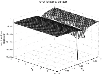
The first test explores the behavior of the error func-tional surface. The variablesxp andRp were
systemat-ically modified over the search space [2.0,8.0]×[0.1,0.4] in a regular mesh of 61×61 = 3721 points. The error functional is calculated for each positionxp and radius Rp generating the error functional surface, as shown
in the plot of Fig. 3 with error functional axis in log-arithm scale. It is possible to see almost flat regions and a narrow channel that contains a prominent global minimum. These characteristics require a powerful op-timization method to reach the global minimum.
3.2. Test 2 - Applying the Simulated annealing
In this test, we evaluated the performance of the devel-oped program to retrieve the position and radius of the non-conductive region. Since SA algorithm is stochas-tic, its convergence to the actual solution is not always
guaranteed. Therefore, it is necessary to run the pro-gram many times to assess its performance. Also, to make a more careful analysis, we have divided the Test 2 in three parts.
In the first part, Test 2.a, the intent was to find only the centerx-coordinate of the non-conductive re-gion. We set the prospective inclusion radius equal to the actual one (Rp = 0.3). The initial solution
of xp was generated randomly in the range [1.0,9.0]
and, to generate a new solution x(pi+1) from the
pre-vious one x(pi) by Eq. (13), it was chosenλ = 0.8. In
the second one, Test 2.b, the program searched only the non-conductive region radius. In this case, we set the prospective inclusion center x-coordinate equal to the actual one (xp = 7.0). The initial solution of Rp
was generated randomly, but in the range [0.05,0.45]. The new solutionR(pi+1)from the previous oneR(pi)by
Eq. (13) was generated consideringλ= 0.04. For both, Test 2.a and Test 2.b, the program was executed consid-ering 1000 iterations, withk= 1, and we set α= 0.95 andTo= 1000.
Finally, the third part, Test 2.c, considers the search for both, position and radius. In this case, we joined the two programs used in the previous parts in a sin-gle one. More specifically, in each iteration (at each temperature) the program carried out two separated searching, one for the position and another for the ra-dius. Due the difficulty to carry out the optimization searching with two variables, we adopted 2000 itera-tions, withk= 1, andα= 0.97. As the previous parts, we setT0 = 1000, λ= 0.8, to generate a newxp, and λ= 0.04, to generate a new Rp. Again, the initial
so-lutions of xp and Rp were generated randomly in the
same ranges of the previous parts.
2 3
4 5
6 7
8 0.1 0.15
0.2 0.25
0.3 0.35
0.4 1E−25
1E−20 1E−15 1E−10 1E−5 1
R
p error functional surface
x
p
error functional (log sc ale)
Figure 3 - Error functional surface in logarithm scale. It presents almost flat regions and a channel that contains a prominent global minimum.
found in each one was stored. Table 1 shows the min-imum, maxmin-imum, mean and standard deviation of the final solutions considering all of the runnings for each part. For the best running of the Test 2.c, the solution found was xp = 7.0005 and Rp = 0.3000, with error
functional of 2.6×10⁻¹⁷. For the best running, the evolution of the error functional, the prospective cen-terx-coordinate and the prospective radius during the optimization process are shown in Fig. (4).
0 200 400 600 800 1000 1200 1400 1600 1800 2000 1E−18
1E−16 1E−14 1E−12 1E−10 1E−8 1E−6 1E−4
1E−2 error functional X iteration
iteration t
error functional
(log scale)
(a)
1 2 3 4 5 6 7 8 9
0
200
400
600
800
1000
1200
1400
1600
1800
2000
propective inclusion center x−coordinate X iteration
x
p
iteration t
(b)
0.05 0.1 0.15 0.2 0.25 0.3 0.35 0.4 0.45 0
200
400
600
800
1000
1200
1400
1600
1800
2000
propective inclusion radius X iteration
Rp
iteration t
(c)
Figure 4 - Evolution with the iteration for the best running of Test 2.c of the (a) error functional (b) prospective centerx-coordinate
and (c) prospective radius.
Table 1 - Minimum, maximum, mean and standard deviation of the final solutionsxp and/orRpfor the three parts of the Test
2, considering 50 runnings.
Test 2.a Test 2.b Test 2.c
x
p Rp xp Rp
Min 6.9925 0.2995 6.8388 0.2445
Max 7.0081 0.3005 7.5467 0.3163
Mean 7.0000 0.3001 7.1203 0.2876
Std 0.0032 0.0002 0.2053 0.0214
4.
Discussion and conclusion
We have presented to students the electrical impedance tomography technique and the application of retrieving the size and position of an non-conductive inclusion in-side of a conductive wire using the boundary element method and simulated annealing algorithm. Numeri-cal simulations assessed either the behavior of the error functional in the search-space and the performance of the implemented program. The results show that the problem has a difficult error surface to be optimized. Despite this, the implemented program has presented a satisfactory accuracy to find the non-conductive region. Finally, the presented algorithms and methods have a wide scope of application and should be better appre-ciated in topics of undergraduate and graduate physics programs.
Acknowledgments
ASM acknowledges Conselho Nacional de Desenvolvi-mento Cient´ıfico e Tecnol´ogico (CNPq) (305738/2010-0). VR acknowledges Funda¸c˜ao de Amparo `a Pesquisa do Estado de S˜ao Paulo (FAPESP) (2008/01284-4).
References
[1] R.P. Henderson and J.G. Webster, IEEE Transactions on Biomedical Engineering25, 250 (1978).
[2] W. Lionheart, N. Polydorides and A. Borsic, Electri-cal Impedance Tomography: Methods, History, and Ap-plications, (Institute of Physics Publishing, Bristol, 2005), Chap. The reconstruction problem.
[3] J.F. Abascal, S.R. Arridge, D. Atkinson, R. Horesh, L. Fabrizi, M.D. Luca, L. Horesh, R.H. Bayford and D.S. Holder, NeuroImage43, 258 (2008).
[4] A. Osella, G. Chao and F. Sanchez, American Journal of Physics69, 455 (2001).
[5] L. Borcea, Inverse Problems18, R99 (2002).
[6] A.I. Nachman, The Annals of Mathematics, Second Se-ries143, 71 (1996).
[7] O.H. Menin and V. Rolnik, International Journal of Modern Physics C22, 825 (2011).
[9] D. Goldberg,Genetic Algorithms in Search, Optimiza-tion and Machine Learning(Addison-Wesley Longman Publish, Boston, 1989).
[10] T.C. Martins, E.D.L.B. Camargo, R.G. Lima, M.B.P. Amato and M.S.G. Tsuzuki, in Engineering in Medicine and Biology Society, EMBC, 2011 Annual In-ternational Conference of the IEEE (2011).
[11] H. Kim, C. Boo and Y. Lee, International Journal of Control, Automation and System2, 211 (2005).
[12] V. Rolnik, O.H. Menin, G.L.C. Carosio and P.J. Se-leghim, in ABCM Symposium Series in Mechatronics, Vol. 4 (2010) pp. 835–843.
[13] R. Duraiswami, K. Sarkar and G.L. Chanine, Engineer-ing Analysis with Boundary Elements, 13(1998).
[14] C.A. Brebbia and J. Dominguez,Boundary Elements Methods An Introductory Course, 2nd ed. (Computa-tional Mechanics Publications Southampton Boston, 1992).
[15] W.T. Ang,A Beginner’s Course in Boundary Element Methods (Universal Publishers, Boca Raton, Florida, 2007).
[16] E. Mylott, R. Klepetka, J.C. Dunlap and R. Widen-horn, European Journal of Physics32, 1227 (2011).
[17] N. Metropolis, A. Rosenbluth, M. Rosenbluth, A. Teller and E. Teller, Journal of Chemistry Physics
21, 1087 (1953).