Intrinsic Time-Uncertainties and Decoherence:
Comparison of 4 Models
Lajos Di´osi
Research Institute for Particle and Nuclear Physics, H-1525 Budapest 114, POB 49, Hungary Received on 11 February, 2005
Four models of energy decoherence are discussed from the common perspective of intrinsic time-uncertainty. The four authors — Milburn, Adler, Penrose, and myself — have four different approaches. The present work concentrates on their common divisors at the level of the proposed equations rather than at the level of the interpretations. General relationships between time-uncertainty and energy-decoherence are presented in both global and local sense. Global and local master equations are derived. (The local concept is favored.)
I. INTRODUCTION
Let me begin with an incomplete list of people who formu-lated ideas reformu-lated to the possible role of time or space-time uncertainties in the destruction of quantum coherence. Cer-tainly Feynman [1] mentioned the idea first, and a Hungarian group [2–4] developed a first vague model. From Penrose to Steve Adler and during twenty years, many independent in-vestigations [5–19] shared the central idea and disagreed on the motivations. In the rest of the present contribution I single out four authors: Penrose [5], myself [8, 9], Milburn [12, 13], and Adler [19]. They have four different motivations: Penrose exposes the conceptual uncertainty of location in space-time, I attribute an ultimate uncertainty to the Newtonian gravita-tional field, Milburn assumes that Planck-time is the smallest time, and Adler derives quantum theory in the special limit of a hypothetic fundamental dynamics. The four authors also have four different mathematical apparatuses, four different interpretations, metaphysics, e.t.c., but the four models have common divisors and my present intention is to find and em-phasize them. The reader shall see that the Milburn master equation is identical to the simplest effective equation derived by Adler in his dynamical theory, and Penrose’s equation is a special case of my master equation.
II. ENERGY DECOHERENCE
Decoherence means the destruction of interference. When it happens to energy eigenstates, we talk about energy deco-herence. Decoherence diminishes coherent dispersion like∆E in case of energy decoherence. Too large coherent dispersions mean that the system exhibits strong quantum features. On the contrary, if the coherent dispersions are reasonably small the system looks like a classical one. Since decoherence can diminish coherent dispersions we think that decoherence is instrumental in the emergence of classicality in quantum sys-tems [20]. Decoherence of various observables may be corre-lated or anti-correcorre-lated. Decoherence of thelocalenergy will induce decoherence of location of massive objects. There is no definite rule as to what observable is the primary one to induce decoherence of the others and to cause eventual clas-sicality of the macroscopic variables. There is no apriori rule as to what are the macroscopic observables and what is the threshold for classically small dispersions. Yet, a consistent
decoherence model, even if it is phenomenological, would make suggestions for the primarily decohering observables and for the dynamics of their dispersions. Total energy is a possible choice to start with, and it leads us to the concept of local energies as the primarily decohering observables. En-ergy decoherence has intimate relationship with the intrinsic uncertainty of time, elucidated below in subsections II A and II B.
FIG. 1: Decoherence destroys large quantum fluctuations of total energy.
Decoherence is, similarly to many other irreversible mech-anisms, fueled by the complexity of the exact dynamics, like in the Adler theory (Sec.IV). The other three theories dis-cussed later in Secs.III,V,VI, derive decoherence from non-dynamic mechanisms. They assume inherent randomness of time. The typical effect is a simple exponential decay of co-herence at a certain decoco-herence time scaletD. This
expo-nential rule has been met by almost all dynamic models as well as by the four ones singled out for the present discus-sion. The Milburn-Adler decoherence-time is on the scale of the Planck-timeτPl, the Di´osi-Penrose theory assumes
non-relativistic decoherence-time. I shall abandon the complex details of these theories and wish to compare them at the level of their ultimate phenomenological equations.
A. Global time uncertainty and decoherence
Let me illustrate the naive phenomenology of energy deco-herence emerging from time uncertainty. For simplicity, sup-pose that the initial state of a quantum system is a superposi-tion of only two energy eigenstates of the total Hamiltonian H:
The evolution of the state in timetreads:
|ψ(t)i=c1exp(−i~−1E1t)|ϕ1i+c2exp(i~−1E2t)|ϕ2i . (2) Following our purposes, we add a certain uncertaintyδttot:
t→t+δt , (3)
and substitute it into the Eq.(2). To be concrete, suppose δt is a Gaussian random variable of zero mean and of dispersion proportional to the mean timetitself:
M[(δt)2] =τt , (4) whereτis a certain scale to measure the strength of time-uncertainties. We can evaluate the evolution of the density matrix:
ρ(t)≡M[|ψ(t)ihψ(t)|] = (5) = |c1|2|ϕ1ihϕ1|+|c2|2|ϕ2ihϕ2|+
+ ©
c⋆1c2exp(i~−1∆Et)M£exp(i~−1∆Eδt)¤|ϕ2ihϕ1|+ + h.c. ª
.
The stochastic mean on the r.h.s. yields: M£
exp(i~−1∆Eδt)¤
=e−t/tD , (6)
which means that the off-diagonal term ofρ(t)decays expo-nentially with the decoherence time
tD= ~2
τ 1
(∆E)2 . (7)
It is easy to see that all off-diagonal elements of a generic initial density matrix would decay exponentially. The com-pact form of the evolution equation contains a typical double-commutator term in addition to the standard double-commutator on the r.h.s. of the von Neumann equation:
dρ dt =−i~
−1[H,ρ]−1 2τ~
−2[H,[H,ρ]] .
(8) The direct proof of this master equation is simple. The reader is referred to the proof of the more general case (12).
I anticipate that the above master equation will be obtained from slightly different concepts. In Sec.III the time uncer-taintyδt follows the Poisson statistics and the Eq.(8) is ob-tained in the proper time-coarse-grained limit. In Sec.IV the Eq.(8) is exactly derived from the uncertainties of the Planck-constant. The corresponding mathematics is trivial. Gaussian randomness δt can mathematically be delegated to the ran-domnessδ~−1since in the solutions of the
Schr¨odinger—von-Neumann equation the Planck-constant and the time appear always in the product form~−1t. For the physics of the above two versions, see Secs.III and IV.
B. Local time uncertainty and decoherence
It is straightforward to consider a local generalization of total-energy decoherence. We drop the concept of global un-certaintyδt of global timetin favor of local uncertaintiesδtr
of the local timetr:
tr→t+δtr , (9)
whererlabels spatial cells. Let, by assumption, theδtr be Gaussian random variables of zero mean and of spatial corre-lation proportional to the timetitself:
M[δtrδtr′] =τrr′t , (10)
whereτis a certain Galileo invariant spatial correlation func-tion. Let us write the total Hamiltonian as the sumH=∑rHr of local ones. The solution of the von Neumann equation takes this form:
ρ(t) =ρ(0) − i~−1
∑
r[Hrtr,ρ(0)]−
− 1
2~
−2
∑
r,r′
[Hrtr,[Hr′tr′,ρ(0)]] , (11)
plus higher order terms int. Let us take the stochastic mean of the r.h.s., usingM[tr] =t andM[trtr′] =τrr′t+t2. This leads to the following master equation att→0:
dρ dt =−i~
−1[H,ρ]−1 2~
−2
∑
r,r′
τrr′[Hr,[Hr′,ρ]] . (12)
Since the matrix τis non-negative the above class of mas-ter equations will, as expected, decohere the superpositions of local-energy eigenstates.
III. MILBURN: DISCRETE TIME UNCERTAINTY
Milburn assumes discrete global time which is of the form nτPl The integer n is random with Poisson distribution of
mean value
M[n] =t/τPl . (13)
Hence time, too, becomes intrinsically uncertain while t stands for the respective mean value of the random time. Mil-burn assumes, furthermore, that the random structure of time is not accessible to us and we can only observe the physics averaged for the random fluctuations of time.
It is straightforward to write down the master equation gov-erning the evolution of the stateρ. First, we write down the change of the state in a single step of the discrete time:
ρ→exp(−i~−1HτPl)ρexp(i~−1HτPl) . (14)
Consider an infinitesimal intervaldtof mean time. During it, the above step occurs with the infinitesimal probabilitydt/τPl,
otherwise the state remains unchanged. Taking the averaged change ofρduringdt, we obtain the Milburn master equation:
dρ dt =
1 τPl
£
exp(−i~−1HτPl)ρexp(i~−1HτPl)−ρ ¤
. (15) Let us expand the r.h.s. upto the first order in the Planck-time:
dρ dt =−i~
−1[H,ρ]−1 2τPl~
−2[H,[H,ρ]] .
TABLE I: Decoherence times for the Milburn master equation.
∆E=1eV (atomic superpositions) tD∼1013s (irrelevant in atomic physics)
∆E=1GeV (high energy superpositions) tD∼10−5s (would be irrelevant for nuclear forces) ∆E=1J (macroscopic superpositions) tD∼10−25s (excludes superposition of macro-energies)
The expansion is valid at the condition∆EτPl ≪~. Recall
that the above equation is identical with Eq.(8) at the choice τ=τPl. Its basic feature is that the off-diagonal elements ofρ
in energy representation will decay at the characteristic deco-herence time (7):
tD= ~2
τPl
1
(∆E)2 . (17) This scale suggests plausible physics, at least at a quick glance. The intrinsic time-uncertainty does practically not de-cohere atomic superpositions, while large energy superposi-tions would decay at extreme short times (Tab.I).
IV. ADLER: EMERGENT QUANTUM MECHANICS
In Adler’s theory, the deepest level of dynamics is classi-cal. The generalized coordinates are complexN×Nhermitian matrices{qr}. Their labelsrcan be taken as, e.g., labels of
spatial cells. The dynamics is defined by the Lagrangian: L[{qr},{q˙r}] =TrL[{qr},{q˙r}] . (18)
It is also called trace Lagrangian, generating trace dynamics forqr. Following the standard method, Adler introduces the
canonical momenta:
pr=
∂L ∂qr
, (19)
and the Hamilton function: H=Tr
∑
r
prq˙r−L . (20)
If the Lagrange functionLis constructed from the generalized coordinatesqr, from the velocities ˙qr, from complex number
coefficients, and we exclude matrix coefficients then we can prove that the following matrix is a conserved dynamic quan-tity [21]:
∑
r[qr,pr] =C˜ =const. (21)
The proof is straightforward. We can write: dC˜
dt = d dt
∑
r· qr,
∂L ∂q˙r ¸
=
∑
r µ·
qr,
∂L ∂qr ¸
+
·
˙ qr,
∂L ∂q˙r
¸
,
(22) where we applied the Euler-Lagrange equation. The r.h.s. vanishes. Indeed, from the unitary invariance of L under,
say, the infinitesimal variationδqr=i[Λ,qr]andδq˙r=i[Λ,q˙r]
whereΛis an arbitrary hermitian matrix, we have: 0=δL=iTr
∑
r µ
[Λ,qr]
∂L ∂qr
+ [Λ,q˙r]
∂L ∂q˙r
. (23)
After cyclic permutations under the trace operation, we recog-nize the r.h.s. of Eq.(22) which must vanish because of the arbitrariness of the hermitian matrixΛ.
The conservation ruledC/˜ dt=0 is classical but it inspires something which looks quantum mechanical. If we were able to prove that each term[qr,pr]of the l.h.s. of Eq.(21) is
con-stant on its own then we would choose those concon-stants asi~
each. Provided furthermore that the choice[qr,ps] =0 is also
possible for allr6=s, we would obtain the structure of Heisen-berg quantum mechanics from the underlying classical ma-trix dynamics. Adler was able to show that the equipartition mechanism of the classical Gibbs-statistical physics will in-deed provide the desired solutions. In a suitablestatistical av-erage, an effective theory emerges with the approximate com-mutation relations:
[qeffr ,peffr ] =δrs×const. (24)
One sets const=i~. The classical dynamics of the effective
variables turns out to be the emergent unitary dynamics: ˙
qeffr =i~−1[Heff,qeff
r ], p˙effr =i~−1[Heff,peffr ] . (25)
Hence, one has derived an emergent quantum-canonical struc-ture and unitary dynamics. Adler exploits that this strucstruc-ture is statistically blurred. At a closer look, the emergent quan-tum mechanics contains some irreversibility. It will be easy to see the resulting master equation in Schr¨odinger represen-tation. We start from the effective von Neumann equation ˙
ρ=−i~−1[Heff,ρ] and we observe that ~ is the statistical mean of a fluctuating parameter. Let us reintroduce the fluc-tuations of~:
~−1→~−1+δ~−1 , (26)
and let us approximate them by a certain white-noise satisfy-ing
M[(δ~−1)2] =~−2τ/t , (27) where the precise meaning ofδ~−1is the fluctuation of~−1’s
average over the periodt. Let us insert Eq.(26) into the von Neumann equation and let us average overδ~−1. The
result-ing master equation reads: dρ
dt =−i~
−1[Heff,ρ]−1 2τ~
−2[Heff,[Heff,ρ]] .
This is again the master equation of energy decoherence. In the light of numerous experimental evidences, Adler gives a detailed analysis of the possible parametrization, in-cluding the natural choiceτ=τPl. To date, this is perhaps the
most complete available discussion of the observable scales of energy decoherence.
On the top of the exact Heisenberg structure (24,25), the trace dynamics is more likely to superpose local fluctuations than global ones. Therefore global fluctuationsδ~−1are re-placed by correlated local fluctuationsδ~−r1. The
correspond-ing master equation will be of the form (12) with the corre-lation matrix yet to be specified from the equilibrium trace dynamics.
V. PENROSE: UNCERTAINTY OF THE POINT-WISE IDENTITY IN SPACE-TIMES
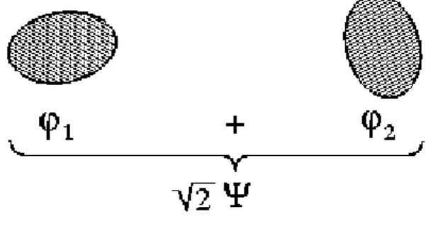
“. . . when the geometries become significantly different from each other, we have no absolute means of identifying a point in one geometry with any particular point in the other . . . , so the very idea that one could form a superposition of the matterstates within these two separate spaces becomes pro-foundly obscure” — this is the geometer’s argument against the concept of sharp geometry. If superpositions of states with very different mass distributions existed they should “decay”. Penrose considers a balanced superposition of two separate
FIG. 2: The superposition of two different mass distributions (lumps), corresponding to separate wave packetsϕ1andϕ2.
wave packets representing two different positions of a massive object (Fig.2). If the massM is large enough, the two wave packets represent two very different mass distributions. Pen-rose postulates the following decay timetD for the balanced
superposition of twolumps:
tD=~/∆Egrav , (29)
whereEgrav is the energy we must, hypothetically, supply to
the system in order to separate the two lumps against gravita-tional forces:
Egrav=|U11+U22−U12| . (30) The quantity Egrav is the Newton self-energiesU11+U22 of the two lumps minus their interaction energyU12.
This is the Penrose proposal. As far as I know, there has been no microscopic definition of the mass distributions of
the lumps which enter the calculation of the Newtonian ener-gies. Penrose assumes the macroscopic density for the lumps and does not resolve it for atomic scales. This way one can calculate the decoherence time for various situations. Since the gravitational self- or mutual energies of atomic systems are very small, the calculatedtD’s will be extremely long. The
atomic superpositions will never decay in the Penrose theory. Massive superpositions, on the other hand, would never be formed because they would decay immediately. If, for ex-ample, one considers a rigid ball of density∼1g/cm3then a plausible critical sizeRcrit∼10−5cm follows, to separate
mi-croscopic from mami-croscopic scales. Its vague interpretation is the following [8]. Let us prepare the ball of radiusRin a wave packet as narrow as∆r∼R. Then we compare the order of dynamical time scale of the wave packet widening with the order of decoherence time (29). We shall see that for small balls (R≪Rcrit) the unitary dynamics dominates while for
large balls (R≫Rcrit) decoherence is quicker and wins over
the unitary dynamics.
Penrose also emphasizes the difference between the unitary evolution and the decay (reduction) of superpositions, denoted byUandRresp., in his works. While the contrary features of Uand Rhave been extensively discussed, the details of evolution during reductionRhave remained unspecified. Re-garding the generic form of state evolution, Penrose writes down the formal sequenceU,R,U,R, . . .while he does not construct a differential evolution equation – master equation – incorporating bothUandR.
VI. DI ´OSI: UNCERTAINTY OF LOCAL TIME
In terms of local time uncertainties (9,10), this theory intro-duces the following universal correlation:
τrr′ =const×
G~ |r−r′|c
−4 , (31)
whereGis the Newton constant andcis the velocity of light. Let me explain the underlying arguments. According to the theory of general relativity, the uncertainties of local time can be represented by the fluctuations of theg00component of the metric tensor. If the average space-time is flat, which we as-sume for simplicity, thenM[g00] =1 and, in Newtonian limit, δg00=−2c−2ΦwhereΦis the Newton potential. The uncer-tainty of local time becomes directly related to the uncertain Newton potentialΦ:
δtr≡δ
Zt
0
dt′g1/200 (r,t′)≈ −c−2
Zt
0
dt′Φ(r,t′) . (32) If we knew the correlation of local uncertainties of the New-tonian gravity, we could calculate the correlation of local time uncertainties. According to heuristic calculations [8, 22], the local gravitational accelerationg=−∇Φhas an inherent un-certainty, totally uncorrelated in space and time:
This implies the following correlation function for the Newton potential:
M[Φ(r,t)Φ(r′,t′)] =const× G~
|r−r′|δ(t−t
′) . (34)
Inserting Eq.(32) intoM[trtr′′]and using Eq.(34), we arrive at
the correlation (31) of local time-uncertainties. Let us em-phasize that the relativistic time-correlation function (31) is equivalent with the non-relativistic gravity-correlation (34). As we shall see, the speed of lightccancels from the quantum master equation.
Now we can derive the master equation valid on the aver-aged space-time. We start from the general equation (12) with the local-time correlation (31). This latter is proportional toc4 which makes it extremely small. In the total energy, it is only the Einstein energy which appreciates the time-fluctuations. We write its local decomposition asc2∑
rf(r)where f(r)is the operator of local mass density. Then we identifyHrin the general master equation (12) byc2f(r), yielding:
dρ
dt = − i~
−1[H,ρ]
(35)
− G
2~
−1Z Z drdr′
|r−r′|[f(r),[f(r ′),ρ]] .
This is the master equation we were looking for. [We replaced ∑r by
R
dr, and ignored the numeric factor on the r.h.s. of Eq.(34).] Observe that the chas been canceled and the re-sult is perfect nonrelativistic. This gives us the hint that we can perform an equivalent nonrelativistic proof of the above master equation, starting from the von Neumann equation
˙
ρ=−i~−1[H−∑rΦ(r,t)f(r),ρ], Taylor-expanding the so-lution uptoO(t2)and calculating the stochastic mean by sub-stituting the gravity-correlation (34).
I am going to show that the above master equation yields exactly the Penrose decay (29,30). Let us start from the bal-anced superposition of the two massive lumps (Fig.2):
ρ=1
2|ϕ1+ϕ2ihϕ1+ϕ2| . (36) We assume that the wave packetsϕ1andϕ1are approximate eigenstates of the mass density operator:
f(r)|ϕni=f¯n(r)|ϕni , n=1,2; (37)
where ¯f1(r)and ¯f2(r)are the (c-number) mass distributions of the two lumps, respectively. Using these functions on the r.h.s. of the master equation (35), we can write the contribution of the double-commutator term to the decay of the interference term between the two lumps into this form:
d
dthϕ1|ρ|ϕ2i=−Egrav~
−1hϕ1|ρ|ϕ2i .
(38) The decay time istD=~/Egravwith
Egrav=
Z Z drdr′
|r−r′|[f¯1(r)−f¯2(r)][f¯1(r
′)−f¯2(r′)] , (39)
i.e., it is completely identical to the Penrose proposal (29,30).
A. Digression
I would like to digress about the status of the model. An earliest criticism came from Ghirardi, Grassi and Rimini [23]. The non-relativistic mass distribution f(r)is a basic ingredi-ent of my model (as well as of Penrose’s). In case of point-like constituents of position operatorrkand massmk, the operator
of mass distribution would be f(r) =∑kmkδ(r−rk). Newton
self-energy would diverge hence my master equation would also diverge. I needed a short length cutoff which I chose to be the nuclear size. The choice was naive, optimistic — and wrong. The authors of Ref.[23] pointed out that the model can not be valid below the scale∼10−5cm and they suggested a higher cutoff. The short-length cutoff ∼10−5cm can most easily be implemented by the corresponding spatial coarse-graining of the mass density f(r). Apart from this modifica-tion, the whole mathematics and physics of the model remains the same; the original master equation needs no reformulation at all.
The Penrose proposal avoids the cutoff-difficulty only be-cause it uses the coarse-grained macroscopic mass density from the beginning, without discussing its microscopic def-inition. What happens to the Penrose model if we extend it for the microscopically structured mass distributions of the two lumps, respectively? It faces the same problem that my model did. To calculate Newtonian self-energies, one needs a short-length cutoff. Where should we get it from? Certainly it may be the phenomenological cutoff 10−5cm imposed by Ghirardi, Grassi and Rimini [23] on my model. Ref.[7] shows Penrose’s awareness of the difficulty as well as his preliminary ideas to circumvent it. I am afraid that the proposed solution can still not stand on its own without defining what happens to the Newtonian interaction at short distances.
May I clarify an important and obvious misunderstand-ing in Ref.[6], also in some subsequent works like, e.g., in Ref.[24]. The claim is that my model differs from Penrose’s because I define the decoherence time through the inverse of the Newton interaction potential:
tD=~/|U12| . (40)
This claim is obviously incorrect. A possible source of the misunderstanding was discovered by the late Jeeva Anandan in 1998 [25]: I had displayed a trivially mistaken version [Eq.(12) in Ref.[8]] of Eq.(39), contrary to the otherwise cor-rect master equation. Yet in the same work I had published the correct equation [Eq.(14)] as well. My longer paper [9] had published correct equations (4.16-17) in coincidence with Penrose’s (29-30), respectively.
superpositions, can not differ from my master equation or, at least, it must build on this master equation.
VII. CONCLUDING REMARKS
The purpose of this ‘review’ was limited. It could not cap-ture all aspects of the chosen four models. Discussion of inter-pretational details was restricted to the minimum. The virtue of my work is that I presented the four models from a common perspective which is intrinsic time-uncertainty. To sketch the four models on the same canvas might cause conflicts with the interpretations of the other three authors themselves. To reduce the risk of misunderstanding, I tried to concentrate on the concrete parts (equations) of the four models. I suggest the interested reader to complete his/her knowledge from the original references.
Let me close this work by another very incomplete list of experimental proposals. Their diversity is spectacular. These proposals mention or suggest that the tiny decoherence
ef-fects, like those predicted by the above discussed theories, might (or should) be detected in the spatial motion of a test body on a satellite [3], in proton decay [27], by atom inter-ferometer [17, 29], in the motion of a nano-mirror [28, 31] or other nano-object coupled to quantum optical devices [32], and in very large interferometers [33]. There are quite recent works [34, 35] particularly concentrating on the experimental aspects of energy decoherence, including local energy deco-herence [36–38]. Without consistent (maybe highly phenom-enological) models, the attractive new experimental options would not be used to target such basic quantum issue as uni-versal decoherence.
VIII. ACKNOWLEDGMENTS
The author is grateful to Hans-Thomas Elze for the idea of the DICE symposiums. I thank Steve Adler for his helpful remarks. This work was partially supported by the Hunarian OTKA Grant No. T49384.
[1] R.P. Feynman,Lectures on gravitation(Caltech, 1962-63). [2] F. K´arolyh´azi, Nuovo Cim. 42A, 390 (1966).
[3] F. K´arolyh´azi, A. Frenkel, and B. Luk´acs, in: Physics as nat-ural philosophy, eds.: A. Shimony and H. Feshbach (MIT, Cam-bridge MA, 1982).
[4] F. K´arolyh´azi, A. Frenkel, and B. Luk´acs, in: Quantum concepts in space and time, eds.: R. Penrose and C.J. Isham (Clarendon, Oxford, 1986).
[5] R. Penrose, Shadows of the mind (Oxford University Press, 1994).
[6] R. Penrose, Gen. Rel. Grav. 28, 581 (1996); reprinted in: Physics meets philosophy at the Planck scale, eds.: C. Callen-der and N. Huggett (Cambridge University Press, Cambridge, 2001).
[7] R. Penrose, Phil. Trans. Roy. Soc. Lond.356, 1927 (1998). [8] L. Di´osi, Phys. Lett. A120, 377 (1987).
[9] L. Di´osi, Phys. Rev. A40, 1165 (1989).
[10] J. Ellis, S. Mohanty, and D.V. Nanopoulos, Phys. Lett. B221, 113 (1989).
[11] J. Ellis, J.S. Hagelin, D.V. Nanopoulos, and M. Srednicki, Nucl. Phys.B241(1984) 381.
[12] G.J. Milburn, Phys. Rev. A44, 5401 (1991).
[13] G.J. Milburn, Lorentz invariant intrinsic decoherence, gr-qc/0308021.
[14] J.L. S´anchez-G´omez, in: Stochastic evolution of quantum states in open systems and in measurement processes, eds.: L. Di ´osi and B. Luk´acs (World Scientific, Singapore, 1993).
[15] A.S. Chaves, J.M. Figuerido and M.C. Nemes, Ann. Phys.231, 174 (1994).
[16] I.C. Percival and W.T. Strunz, Proc. Roy. Soc. Lond. A453, 431 (1997).
[17] W.L. Power and I.C. Percival, Proc. Roy. Soc. Lond. A456, 955 (2000).
[18] S. Roy,Statistical geometry and applications to microphysics
and cosmology(Kluwer, Dordrecht, 1998).
[19] S. Adler,Quantum theory as an emergent phenomenon (Cam-bridge University Press, Cam(Cam-bridge, 2004).
[20] D. Giulini, E. Joos, C. Kiefer, J. Kupsch, I.O. Stamatescu, and H.D. Zeh,Decoherence and the appearance of a classical world in quantum theory(Springer, Berlin, 1996).
[21] A.C. Millard, Princeton University Ph.D. Thesis (1997). [22] L. Di´osi and B. Luk´acs, Ann. Phys.44, 488 (1987).
[23] G.C. Ghirardi, R. Grassi, and A. Rimini, Phys. Rev. A42, 1057 (1990).
[24] J. Christian, in: Physics meets philosophy at the Planck scale, eds.: C. Callender and N. Huggett (Cambridge University Press, Cambridge, 2001).
[25] J. Anandan, private communication. [26] J. Anandan, Found. Phys.29, 333 (1999).
[27] P. Pearle and E. Squires, Phys. Rev. Lett.73, 1 (1994). [28] S. Bose, K. Jacobs, and P.L. Knight, Phys. Rev. 59, 3204
(1999).
[29] B. Lamine, M.T. Jaekel, and S. Reynaud, Eur. Phys. J. D20, 165 (2002).
[30] B.L. Hu and E. Verdaguer, Class. Quant. Grav.20, R1 (2003). [31] W. Marshall, C. Simon, R. Penrose, and D. Boumeester, Phys.
Rev. Lett.91, 130401 (2003).
[32] C. Henkel, M. Nest, P. Domokos, and R. Folman, Phys. Rev. A70, 023810 (2004).
[33] G. Amelino-Camelia, Phys. Rev. D62, 024015 (2000). [34] C. Simon and D. Jaksch, Phys. Rev. A70, 052104 (2004). [35] P. Pearle, Phys. Rev. A69, 42106 (2004).
[36] A. Bassi, E. Ippoliti, and S.L. Adler, Phys. Rev. Lett. 94, 030401 (2005).