Fluctuations, Classical Activation, Quantum Tunneling,
and Phase Transitions
D. L. Stein
Departments of Physics and Mathematics, University of Arizona, Tucson, AZ 85721 USA Received on 20 November, 2004
We study two broad classes of physically dissimilar problems, each corresponding to stochastically driven escape from a potential well. The first class, often used to model noise-induced order parameter reversal, comprises Ginzburg-Landau-type field theories defined on finite intervals, perturbed by thermal or other classical spatiotemporal noise. The second class comprises systems in which a single degree of freedom is perturbed by both thermal and quantum noise. Each class possesses a transition in its escape behavior, at a critical value of interval length and temperature, respectively. It is shown that there exists a mapping from one class of problems to the other, and that their respective transitions can be understood within a unified theoretical context. We consider two applications within the first class: thermally induced breakup of monovalent metallic nanowires, and stochastic reversal of magnetization in thin ferromagnetic annuli. Finally, we explore the depth of the analogy between the two classes of problems, and discuss to what extent each case exhibits the characteristic signs of critical behavior at a sharp second-order phase transition.
I. INTRODUCTION
Noise-induced escape from a locally stable state governs a wide range of physical phenomena [1]. In spatially extended classical systems, where the noise is typically, but not nec-essarily, of thermal origin, these phenomena include homo-geneous nucleation of one phase inside another [2], micro-magnetic domain reversal [3, 4], pattern formation in non-equilibrium systems [5], and many others. The concepts and techniques employed are formally identical to those used in tunneling problems in quantum field theories, including among others the ‘decay of the false vacuum’ [6], anomalous particle production [7], and macroscopic quantum tunneling in a dc SQUID [8].
Recently a new kind of ‘phase transition’, in the classical activation behavior of spatially extended systems perturbed by weak spatiotemporal noise, has been uncovered and ana-lyzed [9–11]. The existence of a similar crossover, from ther-mal activation to quantum tunneling in systems as simple as a single degree of freedom, has long been known [12–22]. Here we will review the stochastic escape behaviors of both types of systems, explore the depth of the analogy between them, discuss to what extent the crossover can be thought of as a type of second-order phase transition, and show how the purely classical transition, occurring as system length is var-ied, can shed light on the crossover from classical activation to quantum tunneling as temperature is lowered. But let’s begin with a purely classical problem.
II. MODEL
Consider an extended system described by a classical field φ(z,t) defined on the spatial interval [−L/2,L/2], subject to the potentialV(φ)and perturbed by spatiotemporal white noise. Its time evolution is governed by the stochastic Ginzburg-Landau equation
∂tφ=∂zzφ−∂φV(φ) +
√
2Tξ(z,t), (1)
where all dimensional quantities have been scaled out. The first term on the RHS arises from a field ‘stiffness’, i.e., an energy penalty for spatial variation of the field. The system is stochastically perturbed by additive white noiseξ(z,t), sat-isfyinghξ(z1,t1)ξ(z2,t2)i=δ(z1−z2)δ(t1−t2). We consider only weak noise, i.e., the noise magnitudeT is small com-pared to all other energy scales in the problem (formally, our analysis will be asymptotically valid in theT →0 limit). The frictional coefficient has been set to one, so whenT is temper-ature Eq. (1) obeys the fluctuation-dissipation relation.
The deterministic, or zero-noise, dynamics can be written as the variation of an action
H
with the fieldφ:˙
φ=−δ
H
/δφ, (2) and because the dynamics is gradient, the actionH
is simply an energy functionalH
[φ]≡Z L/2
−L/2 dz
· 1 2(∂zφ)
2+V(φ)¸.
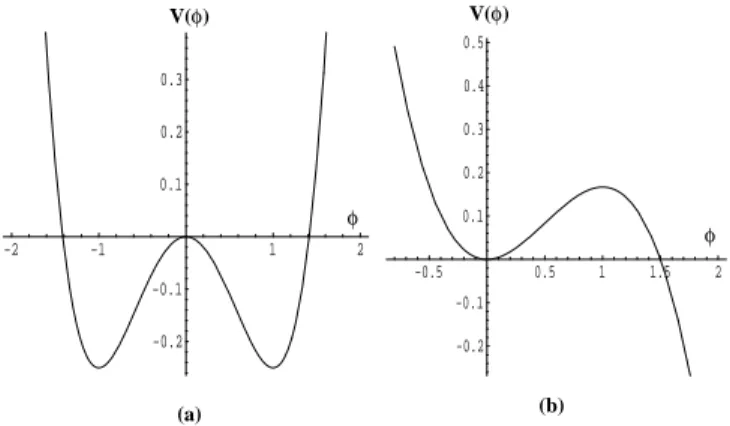
(3) We will mostly consider relatively simple potentials, in par-ticular the symmetric bistable quartic potential
Vs(φ) =−1 2φ
2+1 4φ
4,
(4) and the asymmetric monostable cubic potential
Va(φ) =1
2φ 2−1
3φ
3. (5)
Both potentials are shown in Fig. 1.
In the weak-noise (T→0) limit, the classical activation rate for a transition out of a stable well is
V(φ) V(φ)
-2 -1 1 2
-0.2 -0.1 0.1 0.2 0.3
-0.5 0.5 1 1.5 2
-0.2 -0.1 0.1 0.2 0.3 0.4 0.5
(a) (b)
φ
φ
FIG. 1: Potentials used in discussion: (a) bistable quartic (Eq. (4)) and (b) monostable cubic (Eq. (5)).
III. THE INFINITE-DOMAIN CASE
Let’s start by considering theL=∞case, which was fully worked out for the classical nucleation problem by Langer [2] and for the quantum tunneling problem by Callan and Cole-man [6]. (See also SchulCole-man [23] for a good pedagogic treat-ment.) For illustrative purposes, we will use the bistable quar-tic potential (4).
The states of interest — i.e., the stable and saddle field configurations — are time-independent solutions of the zero-noise Ginzburg-Landau equation ˙φ=−δ
H
/δφ. They are therefore extrema of the action so in the current case satisfy the nonlinear differential equationφ′′=−φ+φ3. (7) Its spatially uniform solutions are just the stable statesφ(z) =
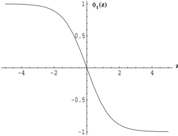
±1 and the local maximumφ=0. But our main interest is in the soliton-like pair (or ‘bounce’ [6])
φ(z) =±tanhh(z−z0)/ √
2i (8)
wherez0is a constant whose presence denotes the fact that the ‘domain wall’, i.e. the spatially varying piece of (8) that separates the two stable states, can nucleate anywhere on the line.
Assuming for the moment that (8) is the saddle config-uration (this will be justified below), the activation energy ∆E =E[φsaddle]−E[φstable] in the Kramers rate formula (6) can be computed, giving
∆E=
Z ∞
−∞dz
h1
2(∂zφsaddle)
2+V(φsaddle)i
−
Z ∞
−∞
dzh1
2(∂zφstable)
2+V(φstable)i=2 √
2
3 , (9)
which is essentially the energy of a single domain wall. In order to compute the prefactorΓ0of the Kramers rate (6), we need to examine fluctuations about the optimal escape path, in particular in the vicinity of the stable and saddle field
(z) φ
-6 -4 -2 2 4 6
-1 -0.5 0.5 1
z
FIG. 2: The ‘bounce’ described by Eq. (8) withz0=0. For clarity,
only one of the symmetric pair is shown.
configurations. The procedure for doing this is described in detail elsewhere (see, for example, [11, 23, 24]), and will be simply summarized here.
Let ϕs denote the stable state (in this case, the uniform ±1 state), and letϕt denote the transition (saddle) state (here
given by Eq. (8)). Consider a small perturbationηabout the stable state, i.e.,ϕ=ϕs+η. Then to leading order ˙η=-Λsη,
whereΛsis the linearized zero-noise dynamical operator
gov-erning the time evolution of fluctuations aboutϕs. Similarly
Λtis the linearized zero-noise dynamical operator forϕt.
We next diagonalize the linear time-evolution operators, by decomposing fluctuations about the stable and transition states into normal modes, which are eigenfunctionsηiof the
corre-sponding operators:
Λbηi=λiηi, (10)
whereb=s,t. An eigenfunction with positive eigenvalueλi>
0 is a stable mode; one withλi<0 is unstable. A stable (or
metastable) state therefore has allλi>0; a saddle state has
a singleλi<0. Its corresponding eigenfunction denotes the
unstable direction (in function space) in the vicinity of the saddle, leading either back to the initial stable configuration or out of the well entirely. With the potential (4), the eigenvalue equation becomes
˙
η=−Λbη≡ −£−d2/dz2+ (−1+3φ2b)
¤
η. (11) In most cases the barrier is locally quadratic: all eigenval-ues are nonzero and we’re left with an infinite set of decou-pled quadratic fluctuations about the stable and saddle states. Then [24, 25]
Γ0= 1
2π s
¯ ¯ ¯ ¯
detΛs
detΛt
¯ ¯ ¯ ¯|
λt,0|, (12)
whereλt,0is the only negative eigenvalue ofΛt. In general,
of an infinite number of eigenvalues with magnitude greater than one. However, theirratio, which can be interpreted as the limit of a product of individual eigenvalue quotients, is finite.
There is a technical difficulty that has not yet been ad-dressed, namely the existence of asoft collective mode cor-responding to the arbitrariness ofz0in (8): the domain wall (or ‘instanton’) can nucleate anywhere. The resulting transla-tional symmetry implies a zero-eigenvalue mode. Its removal can be achieved with the McKane-Tarlie regularization pro-cedure [26] (see also [27]) for functional determinants. This will not be discussed further here, except to note that its pres-ence results, among other things, in a non-Arrhenius (noise-dependent) prefactor that scales with the length. The overall result for the prefactorper unit lengthis then
Γ0/L=³4
√ 6 π
´³ 2 √
πT ´
, (13)
where the first term on the RHS follows from the computation of Eq. (12) with the zero eigenvalue removed via the McKane-Tarlie procedure, and the second term (divided through by length L) gives the contribution of the zero eigenvalue, i.e., the effect of the translational symmetry of the bounce.
IV. THE FINITE-DOMAIN CASE
The differences between the infinite and finite-line cases are not only quantitative; there are important qualitative dif-ferences that are also relevant, in an entirely different context, to the classical ↔quantum crossover (Sec. VI). The most striking of these differences is a sharp change in activation behavior as interval length is varied; moreover, this change exhibits characteristics of a second-order phase transition [9– 11], but only in a strictly asymptotic sense.
Because we are now working on an interval of finite length, we need to specify boundary conditions. With the exception of the zero-energy mode that accompanies only translation-invariant (such as periodic) boundary conditions, different choices of boundary conditions lead only to minor quantita-tive differences. To avoid the (minor) complication of the zero mode altogether, we will employ Neumann boundary conditions: ∂φ/∂L|−L/2=∂φ/∂L|L/2=0. With this choice φstable=±1, as before. We will continue to use the notation of Sec. III, whereφs(φt) refers to the stable (transition) state.
For the symmetric φ4 potential with Neumann boundary conditions, the change in activation behavior arises from a bifurcationof the transition state, from a uniform configura-tion below a critical lengthLcto a pair of degenerate, spatially
varying ‘bounce’ configurations aboveLc. More precisely, the
saddle states are
φt=0 (14)
whenL<Lcand
φt=±
r 2m 1+msn(
x √
m+1|m), (15)
φt(z)
-4 -2 2 4
-1 -0.5 0.5 1
z
FIG. 3: The transition stateφt(z)forL=10 (corresponding tom=
0.986) described by Eq. (15). As in Fig. 2, only one of the symmetric pair is shown.
whenL≥Lc, where sn(· |m)is the Jacobi elliptic sn
func-tion with parameter 0≤m≤1. Its quarter-period is given byK(m), the complete elliptic integral of the first kind [28], which is a monotonically increasing function ofm. Asm→ 0+,K(m)decreases toπ/2, and sn(· |m)→sin(·). In this limit the saddle state smoothly degenerates to theφ=0 configura-tion. Asm→1−, the quarter-period increases to infinity (with a logarithmic divergence), and sn(· |m)→tanh(·), the (non-periodic) single-kink sigmoidal function. The Langer/Callan– Coleman bounce solution (8) is thereby recovered asL→∞.
The value ofmin (15) is determined by the interval length Land the Neumann boundary conditions, which require that
L/√m+1=2K(m). (16) The critical length is determined by (16) whenm=0; that is, Lc=π. As previously noted,m→1 corresponds toL→∞,
and the activation energy smoothly approaches the asymptotic value of 2√2/3. The transition state for an intermediate value ofm, corresponding toL=10, is shown in Fig. 3.
The activation energy∆Ecan be solved in closed form for allL>Lc(belowLc, it is simplyL/4):
∆E= 1
3(1+m)3/2 h
4(1+m)E(m)−1
2(1−m)(3m+5)K(m) i
,
(17) with E(m) the complete elliptic integral of the second kind [28]. The activation energy as a function ofLis shown in Fig. 4. Note that the curve of∆Evs.Land its first deriva-tive are both continuous atLc; the second derivative, however,
is discontinuous, as might be expected of a second-order-like phase transition.
A more profound manifestation of critical behavior atLcis
exhibited by the rate prefactorΓ0. When L<Lc=π, both
∆E
2 4 6 8 10 12 14
0.2 0.4 0.6 0.8
L
FIG. 4: The activation energy ∆E as a function of the interval lengthL, for the potential given by Eq. (4) (with all coefficients set equal to one) and Neumann boundary conditions. The dashed line indicates the critical interval lengthLc=πat which the saddle state
bifurcation takes place.
It is immaterial which of the two (degenerate) stable states is used; the eigenvalue spectrum is the same at both because of the symmetry underφ7→ −φ. Linearizing around either stable state yields the operator
Λs=−d2/dz2+2, (18)
and similarly
Λt=−d2/dz2−1. (19)
The eigenvalue spectrum ofΛswith Neumann boundary
con-ditions is
λs,n=2+
π2n2
L2 n=0,1,2. . . (20) The eigenvalue spectrum ofΛt is similarly
λt,n=−1+
π2n2
L2 n=0,1,2. . . . (21) As required, all eigenvalues ofΛsare positive, whileΛthas a
single negative eigenvalueλt,0=−1. Its eigenfunction, which is spatially uniform, is the direction in configuration space along which the optimal escape trajectory approachesφt.
Putting everything together, we find the Neumann-case rate prefactor whenL<Lcto be
Γ0 = 1
2π v u u u t
∏∞n=0 ¡
2+π2n2 L2
¢
¯ ¯ ¯∏
∞ n=0
¡
−1+π2Ln22
¢¯¯ ¯
= 1
23/4π s
sinh(√2L)
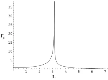
sinL . (22)
1 2 3 4 5 6 7
5 10 15 20 25 30 35
Γ0
L
FIG. 5: Rate prefactorΓ0 for the quartic potential with Neumann
boundary conditions, showing the power-law divergence of the pref-actor asL→L±c.
AsL→L−c(=π−),Γ0∼(L
c−L)−1/2. This divergence has
a simple physical interpretation: the optimal escape trajectory becomes transversally unstable, in the direction defined by the eigenmodeη1, as the critical length is approached. Mathemat-ically the divergence is caused byλt,1→0+asL→L−c.
WhenL>Lc, there are two transition states, namely the
nonuniform bounce configurations±φt given by (15). The
associated linearized evolution operator, computed from (11), is
Λt=− d2 dz2−1+
6m 1+msn
2µ x √
m+1 ¯ ¯ ¯m
. (23) Calculation of the associated determinant quotient, and the single unstable eigenvalueλt,0, is described in detail in [10],
to which the interested reader is referred. The Neumann-case rate prefactor whenL>Lcis
Γ0= 1
π ¯ ¯ ¯ ¯
1− 2 1+m
p
m2−m+1 ¯ ¯ ¯ ¯
× s
sinh(√2L)
√
2|(1−m)K(m)−(1+m)E(m)|. (24) Asm→0+(L→L+c),Γ0∼(L−Lc)−1/2. The prefactor over the entire range ofLis shown in Fig. 5.
The divergence atLcis striking, but requires interpretation.
We defer further discussion to Sec. VII, and turn now to phys-ical applications of the methods and results presented in this section.
V. TWO APPLICATIONS
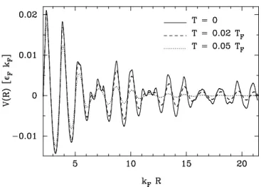
FIG. 6: Electron-shell potentialVshell(R)at three temperatures,
com-puted from the free-electron model of Ref. [36].
A. Lifetimes of monovalent metallic nanowires
Metallic nanowires are cylindrically-shaped incompress-ible electron fluids with diameters of order tens of atoms and with lengths hundreds to thousands of atoms. They are stabilized by quantum shell effects [29–31] but at nonzero temperatures are only metastable, with breakup probably due to thermal fluctuations [32–34]. We have proposed [35] a self-consistent continuum approach to studying the lifetimes of monovalent metallic nanowires, with a large-deviation-induced ‘collapse’ modelled through a stochastic Ginzburg-Landau field theory, of the kind discussed above. Our theory provides good quantitative agreement with available data on nanowire lifetimes, and accounts for the observed difference in stability between alkali and noble metal nanowires.
We treat a nanowire as a cylinder of length L and ra-dius R(z) =R0+φ(z), with z∈[−L/2,L/2]. Radius fluc-tuations are governed by the stochastic Ginzburg-Landau equation (1), whereV(φ) arises from the zero-temperature electron-shell potential of Fig. 6.
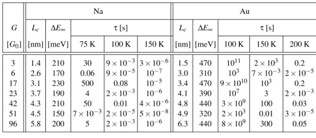
Details of the calculations appear in [35]; here we simply summarize the results, which appear in Table I.
The lifetimes tabulated for sodium nanowires in Table I exhibit a rapid decrease in the temperature interval between 75K and 100K. These lifetimes correlate well with the ob-served temperature dependence of conductance histograms for sodium nanowires [32–34]. A comparison of the lifetimes of sodium and gold nanowires listed in Table I indicates that gold nanowires are much more stable. In our model this arises from the difference in surface tension: σAu=5.9σNa, and is consistent with the observation that noble metal nanowires are much more stable than alkali metal nanowires.
There is also an important prediction contained in Table I, namely that nanowire lifetimes, which exhibit significant vari-ations from one conductance plateau to another, do not vary systematically as a function of radius. It can be seen from Ta-ble I that the activation barriers vary by only about 30% from
one plateau to another, and that a wire with a conductance of 96G0has essentially the same lifetime as that with a conduc-tance of 3G0. In this sense, the activation barrier variation ex-hibitsuniversal mesoscopic fluctuations: in any conductance interval, there are very short-lived wires (not shown in Table I) with very small activation barriers, while the longest-lived wires have activation barriers of a universal size:
0 <∆E∞.0.7
µ~2σ me
¶1/2
, (25)
The derivation of (25) will be presented elsewhere [37]. At present, lifetimes of wires shorter thanLchave not been
systematically studied. We expect that over the next several years the technology will improve to the point where this will become possible, and our predictions for a transition in both activation barriers (from barriers essentially independent of length to those varying linearly with length, as in Fig. 4) and prefactors (Fig. 5) can be tested.
B. Magnetic reversal in nanomagnets
The dynamics of magnetization reversal in submicron-sized, single-domain particles and thin films is important for information storage and other magnetoelectronic applications. This problem can be treated with the methods used through-out this paper, but with a more complicated equation of mo-tion than (1). The magnetizamo-tion dynamics is governed by the Landau-Lifschitz-Gilbert equation [38] perturbed by weak spatiotemporal noise:
∂tM=−γ[M×Heff] + (α/M0)[M×∂tM], (26)
whereM0 is the magnitude of the magnetization M, α the damping constant, andγ>0 the gyromagnetic ratio. The ef-fective fieldHeff=−δE/δMis the variational derivative of the total energyE, which is given by (with free space perme-abilityµ0=1):
E[M(x)] = λ2
Z
Ωd
3x
|∇M|2+1
2
Z
R3d
3x |∇U|2 −
Z
Ω
d3xHe·M, (27)
where Ω is the region occupied by the ferromagnet, λ is the exchange length, andU (defined over all space) satisfies ∇·(∇U+M) =0. The first term on the RHS of (27) is the bending energy, the second the magnetostatic energy, and the last the Zeeman energy. We takeHekθ, using cylindrical co-ˆ ordinates(rˆ,θ,ˆ zˆ). The magnetostatic energy is nonlocal and gives rise to shape anisotropies (for ‘soft’ magnetic materials, like fcc Co or permalloy, crystalline anisotropies are negligi-ble). The out-of-plane anisotropy energy is especially strong, and forcesMto lie in the plane.
TABLE I: The lifetimeτ(in seconds) for various cylindrical sodium and gold nanowires at temperatures from 75K to 200K. HereGis the electrical conductance of the wire in units ofG0=2e2/h,Lcis the critical length, and∆E∞is the activation energy for an infinitely long wire.
From Ref. [35].
Na Au
G Lc ∆E∞ τ[s] Lc ∆E∞ τ[s]
[G0] [nm] [meV] 75 K 100 K 150 K [nm] [meV] 100 K 150 K 200 K
3 1.4 210 30 9×10⁻³ 3×10⁻⁶ 1.5 470 1011 2×10³ 0.2 6 2.6 170 0.06 9×10⁻⁵ 10−7 3.0 310 103 7×10⁻³ 2×10⁻⁵
17 3.1 230 500 0.08 10−5 3.4 470 9×10¹⁰ 103 0.2 23 3.7 190 4 2×10⁻³ 10−6 4.1 390 107 3 2×10⁻³ 42 4.3 210 50 0.01 4×10⁻⁶ 4.8 440 3×10⁹ 100 0.03 51 4.5 150 7×10⁻³ 2×10⁻⁵ 5×10⁻⁸ 4.9 320 2×10³ 0.01 3×10⁻⁵
96 5.8 200 5 2×10⁻³ 10−6 6.3 440 8×10⁹ 300 0.05
the present problem when both the aspect ratiot/R(ring thick-ness divided by ring mean radius), andλ/R, are sufficiently small. Because of the high energy cost of variations inM0, and because the geometry under consideration admits nonsin-gular solutions for the vector fieldM,M0can be taken to be fixed. The result for the total magnetic energy is then [40]:
E
=Z ℓ/2
0
dsh(∂φ
∂s)
2+sin2φ
−2hcosφi, (28)
whereℓis related to ring circumference,his the external mag-netic field magnitude, and φis the local angle between the in-plane magnetization vector and the local field direction. In (28) energy, length, and field are all dimensionless, normal-ized by a corresponding characteristic quantity determined by various ring parameters.
Eq. (26) and the variational equationHeff=−δE/δMyield a nonlinear differential equation that must be satisfied by any time-independent solution:
d2φ/ds2=sinφcosφ+hsinφ. (29) There are three ‘constant’ (φindependent ofθ) but nonuni-form (m =M/M0 varies with position) solutions for 0≤ h<1: the stable state φ=0 (m=θ); the metastable stateˆ φ=π (m=−θ), and a pair of degenerate unstable statesˆ φ=cos−1(−h), which constitute the saddle for a range of
(ℓ,h). Theφ=0,πsolutions are degenerate whenh=0, and theφ=πsolution becomes unstable ath=1.
We have also found a nonconstant ‘bounce’ solution of (29), which is the saddle for the remaining range of(ℓ,h). It is
φ(s,m) =2 cot−1hdn³s−s0 δ
¯ ¯ ¯m
´sn(
R
|m) cn(R
|m)i
, (30)
where dn(·|m), sn(·|m), and cn(·|m) are the Jacobi elliptic functions with parameterm[28],s0is a constant, and
R
andδare given by
sn2(
R
|m) = 1/m−h/2− (1/2m)qm2h2+4(1−m) (31)
δ2 = m2
2−(m+p
m2h2+4(1−m)). (32) Imposition of the periodic boundary condition yields a rela-tion betweenℓandm:
ℓ=2K(m)δ. (33) Asm→0, dn(x|0)→1, and the bounce solution reduces to the constant stateφ=cos−1(−h). The critical length and field where this occurs are related by
ℓc=πδc=2π/
q 1−h2
c. (34)
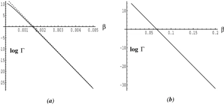
What is interesting here is that the transition is governed by twoparameters: not only the length, but also the magnitude of the externally applied magnetic field. While the former can-not be varied continuously, the latter can, allowing for the first time a detailed experimental probe of the transition. Fig. 7 shows theoretical predictions of the magnetization switching rate at two different field strengths for a ring of fixed circum-ference.
VI. CROSSOVER FROM THERMAL ACTIVATION TO QUANTUM TUNNELING
Only purely classical activation processes have been con-sidered so far, but the transition in activation behavior as in-terval length is increased has an interesting parallel with the crossover from classical activation to quantum tunneling as temperature is lowered. The correspondence can be made ex-plicit by mapping system lengthLin the former case to tem-peratureT in the latter.
logΓ logΓ 0.001 0.002 0.003 0.004 0.005
-25 -20 -15 -10 -5 5 10
0.05 0.1 0.15 0.2
-30 -20 -10 10
(a) (b)
β β
FIG. 7: Total switching rate (in units ofs−1) vs. inverse
tempera-tureβ(in units of◦K−1), at fields of (a) 52.5 mT (nonconstant sad-dle) and (b) 72.5 mT (constant sadsad-dle). Parameters used arek=.01, l=.05,R=200 nm,R1=180 nm,R2=220 nm,M0=8×10⁵A/m
(permalloy),α=.01, andγ=1.7×10¹¹T−1s−1. Deviation of low-field switching rate in (a) from dashed line signals non-Arrhenius behavior. (From Ref. [40].)
whereτ=it is imaginary time, with each path weighted by its Euclidean actionSE[41]:
Z=
Z
D
[q(τ)]exp{−SE[q(τ)]/~}. (35)The integral in (35) runs over all paths periodic in imaginary time, with period~β.
Eq. (35) is derived from the usual definition of the parti-tion funcparti-tion Z=Tr {exp[−β
H
]}, whereH
includes both the systemandits environment. Consequently, even if one is dealing with the tunneling of only a single degree of freedom q(τ), the effects of friction due to its coupling with the envi-ronment must be included. The proper treatment of the effects of damping on quantum mechanical tunneling have been con-sidered by a number of authors; see, for example, [15–18]. Although friction strongly affects the tunneling rate quantita-tively, it will not be included here; this is because our only aim is to present the connection between the transition in thermal activation of (infinite-dimensional) classical fields as length is varied, and the crossover from classical activation to quan-tum tunneling in (one-dimensional) systems as temperature is varied.An early treatment (that ignored dissipation) was given by Goldanskii [12]. Setting the classical, temperature-dependent Arrhenius factor∆E/kBT equal to the zero-temperature
quan-tum tunneling rate through a parabolic barrier, he noted that the characteristic temperature T0 for the quantum tunneling ↔classical activation crossover was
T0=~ωc/(2πkB), (36)
where ωc is the characteristic frequency of the locally
quadratic barrier. Although Goldanskii’s approach led only to an estimate, his formula (36) was quite accurate (in the ab-sence of dissipation), as the following more detailed analy-sis [16–18] will demonstrate (see also [13, 14, 19–22]).
In what follows, we will use the asymmetric potential given by (5). This allows us to consider only incoherent tunnel-ing processes: once the particle tunnels through the barrier,
it escapes for good. A double-well potential such as (4) re-quires consideration of dissipative quantum coherence effects, for which a real-time functional integral approach is better suited (see, for example, [42, 43]). The Euclidean action for a particle of massMis therefore
SE[q(τ)] =
Z β~/2
−β~/2 dτn1
2Mq˙
2(τ) (37)
+ Mhω 2 0 2 q(τ)
2
−λ
3q(τ) 3io+
(frictional terms) where ˙qdenotes a derivative with respect to imaginary timeτ. In the low-friction limit, extremal paths satisfy
−q¨(τ) +ω2
0q(τ)−λq(τ)2=0, (38) with periodic boundary conditionsq(−β~/2) =q(β~/2).
Three extremal solutions are physically relevant. The first is the uniformq(τ) =0 solution, which corresponds simply to the stable state at all temperatures. Of the other two, one is uniform:
qc,+(τ) =ω20/λ (39) and the other is a nonuniform bounce:
qc,−(τ,m) = 3ω2
0 2λ ν(m)
2
dn2³ω0ν(m)
2 (τ−τ0)|m ´
+ ω
2 0 2λ h
1−(2−m)ν(m)2i, (40) where as before 0≤m≤1 and ν(m) = (1−m+m2)−1/4. Imposition of the periodic boundary condition relates the pa-rametermto the inverse temperature:
β=4K(m)/~ω0ν(m). (41) The constantτ0in (40) indicates the translational symmetry in imaginary time arising from the periodic boundary conditions, and corresponds to a zero mode as described in Sec. III.
We can now make explicit the mapping to the thermal acti-vation of classical fields. Here the inverse temperatureβplays the same role as system lengthL in Sec. IV. In particular, high temperature corresponds to the small length regime. For βsmaller than someβc, we would therefore expect the
con-stant solutionqc,+to be the saddle. And indeed it is. The
corresponding action is
SE[qc,+(τ)] =Mω60β~/(6λ2) =β~∆V, (42) where∆V=Mω6
0/(6λ2)is the potential energy difference be-tween the potential barrier top and bottom. Consequently, exp{−SE[qc,+(τ)]/~}=exp[−β∆V], and the classical
Arrhe-nius factor is recovered.
The bounce solutionSE[qc,−(τ)]is the saddle at largeβ. As in Sec. IV, the transition temperatureTcis given by (41) when m→0+. We find thatTc=~ω0/(2πkB), exactly that found by
1/ T
0.5 1 1.5 2 0.2
0.4 0.6 0.8 1 1.2 S(T)
T
5 10 15
-1.2 -1 -0.8 -0.6 -0.4 -0.2
(a) (b)
−S(T)
FIG. 8: (a) The Euclidean action SE[qc(τ)] at all temperatures.
(b) The logarithm of the leading-order escape rate, shown in an Arrhenius-style plot. In both graphs, M=ω0=λ=~=kB=1,
and the dot indicates the crossover.
The action in the low-temperature region
SE[qc,−] =3Mω50/(5λ2(1−m+m2)1/4) ×h2E(m)−[(2−m)(1−m)/(1−m+m2)]K(m)i
+(Mβ~ω6
0/12λ2) h
1−3(2−m)/2p1−m+m2
+(2−m)3/2(1−m+m2)3/2i (43) is, as in the classical field case (cf. Fig. 4), continuous and differentiable at all temperatures; but also as before, its sec-ond derivative is discontinuous. The action, along with the leading-order escape rate, is shown in Fig. 8.
The well-known zero-temperature tunneling rate is recov-ered from (43) in the limit m→1. Summarizing, we find that the classical Arrhenius formula is recovered in the high-temperature limit and the quantum tunneling formula is recov-ered in the zero-temperature limit:
exph−SE(qc,−)/~ i
=
exp[−∆V/kBT] T→∞
exp[−36∆V/5~ω0] T→0 (44)
while in a narrow region aboutT0both contribute.
VII. DISCUSSION
We have demonstrated that in problems involving noise-induced escape of a classical field over a barrier, a type of second-order phase transition, with what appears to be at-tendant critical phenomena (such as power-law divergence of the rate prefactor) occurs as one or more external parameters (length of the interval on which the field is defined, external magnetic field if relevant, and so on) is varied. We have also shown that there is a mathematical mapping of this transition to the classical activation↔quantum tunneling transition for a particle escaping a simple potential well. The mapping here involves identifying interval length (and/or magnetic field, if appropriate) in the classical field case to temperature in the
classical↔quantum case. To avoid confusion, it should be remembered that the asymptotically small parameter is noise strength (typically, but not necessarily, temperature) in the for-mer problem, and Planck’s constant —nottemperature — in the latter.
In this section we will address two questions that immedi-ately come to mind: To what extent can the transitions dis-cussed be considered ‘real’ second-order phase transitions ex-hibiting critical phenomena; e.g., in the sense that the fluctua-tions driving the transition occur on all scales? Secondly, how deep is the correspondence between the classical field transi-tion and the quantum↔classical crossover [13, 14, 16–22]?
A. Is the phase transition ‘real’?
The short answer is: in a mathematically asymptotic sense yes, but from a strictly (and more physically relevant) critical-phenomena-oriented viewpoint, no. Moreover, the observa-tion of rate prefactor divergence depends crucially on the or-der in which relevant parameters (temperature, system length, and so on) are varied. There are clearly different saddle con-figurations, and thereforequalitativelydifferent activation be-haviors, on either side of the transition. But the question we are focusing on here is: what is happening very close to the critical lengthscale? This was extensively discussed in [11], and that discussion will be expanded here.
Naively, the transition appears second-order in several re-spects: the saddle solution is continuous (and even bifurcates in symmetric models such as (4)), and the action is continuous and differentiable at the transition point but has a discontinu-ous second derivative there. But perhaps most compelling, from the point of view of critical phenomena, is the apparent power-law ‘divergence’ of the rate prefactor shown in Fig. 5. We therefore examine this in more detail, first asking what it even means for the prefactor to ‘diverge’.
Of course, at no lengthscale is the actual prefactor infi-nite. Consider the analysis of the noisy symmetric Ginzburg-Landau model given in Sec. IV. It is important to recall that the analysis of the escape rate is, strictly speaking, valid only in an asymptotic sense asT →0: our results applyonly to temperatures sufficiently low so that the escape rate is small.
What the formal divergence of the prefactordoesmean is that the escape behavior becomes increasingly anomalous as Lc is approached, and that it isnon-Arrheniusexactly atLc,
where for allT →0 the prefactor is temperature-dependent, scaling as a negative power ofT. In the region close toLc,
the rate prefactorΓ0is anomalously large, but still finite. The formula (12) — from which the prefactor shown in Fig. 5 was computed — is validonlyforT sufficiently small so that the contributions from the quadratic fluctuations about the rele-vant extremal state of
H
[φ]dominate the action. So as long as all eigenvalues ofΛt are nonzero (excluding, if translationalsymmetry is present, the zero mode which may be extracted), Eq. (12) applies, but only within a temperature region driven to zero asL→Lc. The diminishing size of this region as L→Lc is controlled by the rate of vanishing of the
The implication is that the prefactor behavior depends on whetherT→0 at fixedLnearLc, or whetherLincreases (say)
through Lc at fixed low T. In the former case, one will
re-cover Fig. 5. If instead one fixestemperatureat some small but nonzero value, one should observe first a rising prefactor asL approachesLc, but at someL(depending onT through
a type of ‘Ginzburg criterion’; cf. Fig. 9 in [11]), the prefac-tor crosses over to a non-Arrhenius (temperature-dependent) form. AsLcontinues to increase on the other side ofLc, the
sequence of events is reversed.
The procedure of fixing T and varying L is in many in-stances the more physical one. In this case a correct analy-sis needs to include higher-order (than quadratic) fluctuations about the transition state, as was done, e.g., in [17]. The next higher-order terms will (unless prevented by symmetry) be nonzero. The behavior remains anomalous, however. Suppose one starts to varyLat fixedT, but as soon as non-Arrhenius behavior is encountered, one fixesLand then starts to lower T. A subsequent transition from non-Arrhenius to Arrhenius behavior will again be encountered: asT is lowered, the pref-actor Γ0 rises until it reaches the value shown in Fig. 5; it remains constant thereafter.
Lying behind this description is the relative magnitudes of the thermal energy and that due to quadratic fluctuations in the direction of the eigenmodeη1with vanishing eigenvalue λ1. Non-Arrhenius behavior should be seen at ‘intermedi-ate’ temperatures, where thermal energy is large compared to that due to quadratic fluctuations along theη1direction, but small compared to that arising from higher-order fluctuations. ‘Intermediate’ here depends onL, whose closeness toLc
de-termines the magnitude ofλ1. Arrhenius behavior reappears in the ‘low’ temperature region where the thermal energy is small compared even to that due to the quadratic fluctuations alongη1. And becauseλ1→0 asL→Lc, the crossover from
non-Arrhenius to Arrhenius behavior occurs at an increasingly lower temperature. Exactly atLc, whereλ1is exactly zero, the
escape behavior is non-Arrhenius for allT→0.
There’s an alternative way of describing the situation: when viewed on ‘normal’ fluctuation lengthscales ofO(T1/2), field fluctuations along the eigenmode direction η1 appear to be diverging as L→Lc, accompanied by anomalous transition
behavior. However, when viewed on an ‘anomalous’ length-scale (O(T1/3)orO(T1/4)or ..., depending on the form of the potential), those fluctuations remain finite, and one would pre-sumably observe a rounded maximum of the prefactor (when scaled by the appropriate temperature-dependent factor) atLc.
The situation is therefore fairly subtle; care must be used to describe the ‘transition’ in appropriate terms. Moreover, in perhaps the most important respect, the transition fails a cen-tral test of criticality — that of the disappearance of a char-acteristic fluctuational lengthscale. In our problem, even at Lcthere is a well-defined characteristic lengthscale, albeit an
anomalous one.
This is strikingly different from a similar-looking (on the surface) transition described elsewhere [44–46]. This tran-sition in the activation behavior of non-equilibriumsystems (e.g., where detailed balance is absent in the zero-noise dy-namics) occurs as the result of singularities developing [47]
in the action. These singularities lead in turn to the appear-ance ofcausticsin the pattern of fluctuational trajectories, as in geometric optics. Here the transition occurs as a parameter in the zero-noise dynamics is varied.
In these systems, fluctuations about the optimal escape tra-jectorydo occur at all scales at the critical point, so one cannot simply ‘cure’ the divergence by including higher-order terms as before. Ade novoscaling theory [46, 47] is required. This theory results in an array of nontrivial critical exponents that obeying scaling relations and characterize the divergence (or vanishing) of relevant physical quantities (including, but not limited to, the rate prefactor). Consequently, these non-equilibrium systems can justifiably be said to exhibit true crit-ical behavior at the transition point.
The discussion so far has focused entirely on second-order transitions; what about first-order? This possibility has been discussed by several authors [19–21]. In slightly more com-plicated classical field theories perturbed by spatiotemporal noise, such as a sixth-degree Ginzburg–Landau model, the nonconstant saddle branch of the energy functional
H
[·]can in principle cross the constant saddle branch at a nonzero an-gle. This should give rise to a first-order transition. So, in the phase plane of these models, the second-order transition point (in the limited sense discussed in this section) is presumably the endpoint of a first-order transition curve.B. Is the quantum tunneling↔classical activation crossover for a single degree of freedom identical to the transition in
activation behavior of a classical field on finite intervals?
Mathematically, yes, under the following mapping: Classical↔Quantum Classicalφ4
Small parameter ~ T
Tunable parameter T L
Periodic in β~ L
Here we chose a stochastic Ginzburg-Landauφ4model for specificity, but one can substitute any of the other classical field theories discussed. For the noisy magnetization dynam-ics discussed in Sec. V B, it should be remembered that the transition can occur as either length or field is varied. One also need not choose periodic boundary conditions for classi-cal Ginzburg-Landau field theories; the transition will occur in similar fashion (but with fairly minor differences as described in Sec. IV) with other types of boundary conditions. On the other hand, one is constrained to use boundary conditions pe-riodic inβ~in the quantum↔classical problem.
This mapping is realized when the quantum ↔ classical transition problem is set up using a Euclidean imaginary-time functional integral formulation, in a potential where incoher-ent tunneling dominates. The classical problem is approached similarly as a real-space path integral in the limit of weak spa-tiotemporal noise.
problem — either holding Lfixed and loweringT, or hold-ing T fixed and moving Lthrough Lc. In the first case one
can, in principle, recover the prefactor divergence shown in Fig. 5, while in the second one should observe a sequence of Arrhenius →non-Arrhenius → Arrhenius transition behav-iors, with the width of the non-Arrhenius region vanishing as T →0. ‘Non-Arrhenius’ means, as usual, a prefactorΓ0not determined by (12), and thereby usually aquiring a tempera-ture dependence. In order to see this dependence, one would need to repeat the procedure (fixT, moveLthrough the tran-sition) at several different temperatures.
But in the quantum case, there is no such freedom: here the small parameter,~, cannot be varied. So a prefactor
diver-gence such as Fig. (5) cannot be observed even in principle. In a similar vein, the zero mode arising from the use of pe-riodic boundary conditions will differ in the two cases. This mode arises on the nonconstant (‘bounce’) side of the tran-sition due to translational symmetry — the instanton (or do-main wall) separating the two stable solutions can arise any-where in space (or imaginary time, in the quantum↔ classi-cal case). This leads in turn to aT-dependent (respectively,
~-dependent) prefactor forall L>Lc(respectively,T<Tc).
It should be kept in mind that we have made the im-plicit assumption in the classical field case that temperature
can be lowered to arbitrarily small values. For many sys-tems this may not be the case: either transition rates will become immeasurably low, or the system itself might un-dergo a (real) phase change, or new physics may enter in some other way. Nevertheless, the ability to vary temper-ature does distinguish the classical field transition from the quantum↔classical one. In particular, the magnetic reversal problem (cf. Sec. V B) presents us with the exciting possibil-ity of continuously tuning through the transition by varying an external magnetic field. With the possibility this presents of experimentally studying activation closer to the transition than might otherwise be achieved, we might in this way not only advance our understanding of stochastic reversal in nanoscale magnets, but also uncover new information about the quan-tum↔classical transition that the constancy of~would
oth-erwise prevent us from obtaining.
VIII. ACKNOWLEDGMENTS
This research was partially supported by the U.S. National Science Foundation Grants No. 0099484 and PHY-0351964.
[1] See, for example, J. Garcia-Ojalvo and J.M. Sancho,Noise in Spatially Extended Systems(Springer, New York/Berlin, 1999). [2] J.S. Langer, Ann. Phys.41, 108 (1967); Ann. Physics54, 258
(1969).
[3] L. N´eel, Ann. G´eophys.5, 99 (1949). [4] W. F. Brown, Jr., Phys. Rev.130, 1677 (1963).
[5] M.C. Cross and P.C. Hohenberg, Rev. Mod. Phys. 65, 851 (1993).
[6] S. Coleman, Phys. Rev. D15, 2929 (1977); C.G. Callan, Jr. and S. Coleman, Phys. Rev. D16, 1762 (1977).
[7] G. ’t Hooft, Phys. Rev. D14, 3432 (1976).
[8] C. Morais Smith, B. Ivlev, and G. Blatter, Phys. Rev. B49, 4033 (1994).
[9] R.S. Maier and D.L. Stein, Phys. Rev. Lett.87, 270601 (2001). [10] R.S. Maier and D.L. Stein, inNoise in Complex Systems and Stochastic Dynamics, eds. L. Schimansky-Geier, D. Abbott, A. Neiman, and C. Van den Broeck (SPIE Proceedings Series, v. 5114, 2003), pp. 67–78.
[11] D.L. Stein, J. Stat. Phys.114, 1537 (2004).
[12] V.I. Goldanskii, Dokl. Acad. Nauk SSSR 124, 1261 (1959); 127, 1037 (1959).
[13] I. Affleck, Phys. Rev. Lett.46, 388 (1981). [14] P.G. Wolynes, Phys. Rev. Lett.47, 968 (1981).
[15] A.O. Caldeira and A.J. Leggett, Phys. Rev. Lett.46, 211 (1981); Ann. Phys. (NY)149, 374 (1983);153, 445 (1983) (Erratum). [16] A.I. Larkin and Yu.N. Ovchinnikov, JETP37, 322 (1983). [17] H. Grabert and U. Weiss, Phys. Rev. Lett.53, 1787 (1984). [18] P.S. Riseborough, P. H¨anggi, and E. Freidkin, Phys. Rev. A32,
489 (1985).
[19] E.M. Chudnovsky, Phys. Rev. A46, 8011 (1992).
[20] A.N. Kuznetsov and P.G. Tinyakov, Phys. Lett. B 406, 76 (1997).
[21] D.A. Gorokhov and G. Blatter, Phys. Rev. B56, 3130 (1997).
[22] K.L. Frost and L.G. Yaffe, Phys. Rev. D59, 065013 (1999). [23] L.S. Schulman,Techniques and Applications of Path
Integra-tion(Wiley, New York, 1981), chapter 29.
[24] P. H¨anggi, P. Talkner, and M. Borkovec, Rev. Mod. Phys.62, 251 (1990).
[25] Theory of Continuous Fokker–Planck Systems, edited by F. Moss and P. V. E. McClintock (Cambridge University Press, Cambridge, 1989).
[26] A.J. McKane and M.B. Tarlie, J. Phys. A28, 6931 (1995). [27] H. Kleinert and A. Chervyakov, Phys. Lett. A245, 345 (1998). [28] Handbook of Mathematical Functions, edited by
M. Abramowitz and I. A. Stegun (Dover, New York, 1965). [29] F. Kassubek, C.A. Stafford, H. Grabert, and R.E. Goldstein,
Nonlinearity14, 167 (2001).
[30] C.-H. Chang, F. Kassubek, and C.A. Stafford, Phys. Rev. B68, 165614 (2003).
[31] D.F. Urban and H. Grabert, Phys. Rev. Lett.91, 256803 (2003). [32] A.I. Yanson, I.K. Yanson, and J.M. van Ruitenbeek, Nature400,
144 (1999).
[33] A.I. Yanson, I.K. Yanson, and J.M. van Ruitenbeek, Phys. Rev. Lett.84, 5832 (2000).
[34] A.I. Yanson, J.M. van Ruitenbeek, and I.K. Yanson, Low Temp. Phys.27, 807 (2001).
[35] J. B¨urki, C.A. Stafford, and D.L. Stein, inNoise in Complex Systems and Stochastic Dynamics II, eds. Z. Gingl, J. Sancho, L. Schimansky-Geier, and J. Kertesz, (SPIE Proceedings Series, v. 5471, 2004), pp. 367–379.
[36] C.A. Stafford, D. Baeriswyl, and J. B ¨urki, Phys. Rev. Lett.79, 2863 (1997).
[37] J. B¨urki, C.A. Stafford, and D.L. Stein, in preparation. [38] F.H. deLeeuw, R. van den Doel, and U. Enz, Rep. Prog.
Phys.43, 689 (1980).
Mi-cromagnetics”, Arch. Rat. Mech. Anal., in press. Available at http://www.math.nyu.edu/faculty/kohn.
[40] Kirsten Martens, D.L. Stein, and A.D. Kent, “Magnetic Re-versal in Mesoscopic Ferromagnetic Rings”, submitted to Phys. Rev. Lett.; available as cond-mat/0410561.
[41] R.P. Feynman,Statistical Mechanics(Benjamin, Reading, MA, 1972).
[42] A.J. Bray and M.A. Moore, Phys. Rev. Lett.49, 1545 (1982).
[43] S. Chakravarty and A.J. Leggett, Phys. Rev. Lett.52, 5 (1984). [44] R.S. Maier and D.L. Stein, Phys. Rev. Lett.71, 1783 (1993). [45] M.I. Dykman, M.M. Millonas, and V.N. Smelyanskiy.
Phys. Lett. A195, 53 (1994).
![FIG. 8: (a) The Euclidean action S E [q c (τ)] at all temperatures.](https://thumb-eu.123doks.com/thumbv2/123dok_br/18981458.457180/8.892.81.445.80.272/fig-euclidean-action-s-e-q-τ-temperatures.webp)
