Quantum Chaos, Dynamical Stability and Decoherence
Giulio Casati1,2,3 and Tomaˇz Prosen4 1 Center for Nonlinear and Complex Systems, Universita’ degli Studi dell’Insubria, 22100 Como, Italy
2 Istituto Nazionale per la Fisica della Materia, unita’ di Como, 22100 Como, Italy, 3 Istituto Nazionale di Fisica Nucleare, sezione di Milano, 20133 Milano, Italy,
4 Department of Physics, Faculty of mathematics and physics, University of Ljubljana, 1000 Ljubljana, Slovenia,
Received on 20 February, 2005
We discuss the stability of quantum motion under system’s perturbations in the light of the corresponding classical behavior. In particular we focus our attention on the so called “fidelity” or Loschmidt echo, its rela-tion with the decay of correlarela-tions, and discuss the quantum-classical correspondence. We then report on the numerical simulation of the double-slit experiment, where the initial wave-packet is bounded inside a billiard domain with perfectly reflecting walls. If the shape of the billiard is such that the classical ray dynamics is reg-ular, we obtain interference fringes whose visibility can be controlled by changing the parameters of the initial state. However, if we modify the shape of the billiard thus rendering classical (ray) dynamics fully chaotic, the interference fringes disappear and the intensity on the screen becomes the (classical) sum of intensities for the two corresponding one-slit experiments. Thus we show a clear and fundamental example in which transi-tion to chaotic motransi-tion in a deterministic classical system, in absence of any external noise, leads to a profound modification in the quantum behavior.
I. INTRODUCTION
As it is now widely recognized, classical dynamical chaos has been one of the major scientific breakthroughs of the past century. On the other hand, the manifestations of chaotic mo-tion in quantum mechanics, though widely studied [1, 2], re-main somehow not so clearly understood, both from the math-ematical as well as from the physical point of view.
The difficulty in understanding chaotic motion in terms of quantum mechanics is rooted in two basic properties of quan-tum dynamics:
(1) The energy spectrum of bounded, finite number of par-ticles, conservative quantum systems is discrete. This means that the quantum motion is ultimately quasi-periodic, i.e. any temporal behavior is a discrete superposition of finitely or countably many Fourier components with discrete frequen-cies. In the ergodic theory of classical dynamical systems, such a quasi-periodic dynamics corresponds to the limiting case of integrable or ordered motion while chaotic motion re-quires continuous Fourier spectrum [3].
(2) Quantum motion is dynamically stable, i.e. initial errors propagate only linearly with time [4]. Linear instability is a typical feature of classical integrable systems and this con-trasts the exponential instability which characterizes classical chaotic systems.
Therefore it appears that quantum motion always exhibits the characteristic features of classically integrable, regular motion which is just the opposite of dynamical chaos. How-ever, it has been shown that this apparently paradoxical situ-ation can be resolved with the introduction of different time scales inside which the typical features of classical chaos are present in the quantum motion also. Since these time scales diverge as Planck constant~ goes to zero, no contradiction
arises with the correspondence principle [5].
It has been remarked that, while exponential separation of orbits starting from slightly different initial conditions is asso-ciated to classical chaos, the situation in quantum mechanics is drastically different. Indeed the scalar product of two states
hψ1|ψ2iis time-independent due to unitarity of time evolu-tion. This has led to the introduction of fidelity as a measure of stability of quantum motion [6]. More precisely one con-siders the overlap of two states which, starting from the same initial conditions, evolve under two slightly different Hamil-tonians H andHε=H+εV. The fidelity is then given by f(t) =|hψ|exp(iHεt/~)exp(−iHt/~)|ψi|2. The quantity f(t) can be seen as a measure of the so-called Loschmidt echo: a state|ψievolves for a timet under the (unperturbed) Hamil-tonian H, then the motion is reversed and evolves back for the same timetunder the (perturbed) HamiltonianHεand the overlap with the initial state|ψiis considered.
However, we would like to stress that, in principle, such difference between classical and quantum mechanics actually does not exists. The Liouville equation, which describes clas-sical evolution, is unitary and reversible as the Schr¨odinger equation. However, there exist time scales up to which quan-tum motion can share the properties of classical chaotic mo-tion including the local exponential instability (see, e.g., Ref. [5]). Due to the existence of such time scales, what may be different, and indeed it is, is the degree of stability of dynam-ical motion. Indeed, as clearly illustrated in the analysis of the Loschmidt echoes with respect to variation of the wave-function [4] or variation of the Hamiltonian [7], quantum mo-tion turns out to be more stable than the classical momo-tion.
to classically chaotic systems, the emerging picture which re-sults from analytical and numerical investigations [7, 10–18] is that both exponential and Gaussian decays are present in the time behavior of fidelity. The strength of the perturbation de-termines which of the two regimes prevails. The decay rate in the exponential regime appears to be dominated either by the classical Lyapunov exponent or, according to Fermi golden rule, by the spreading width of the local density of states.
In addition, at least for short times, the decaying behav-ior depends on the initial state (coherent state, mixture, etc.). While it can be true that, for practical purposes, the short time behavior of fidelity may be the most interesting one, it is also true, without any doubt, that in order to have a clear theoretical understanding and identify a possible universal type of quan-tum decay one needs to consider the asymptotic behavior of fidelity. On the other hand, in the regime of very small pertur-bation, which may be of interest for practical quantum com-putation, one may in fact be interested also in the long-time behavior of fidelity in the so-called linear response regime.
This short review is composed of three parts. In section II we discuss the problem of classical fidelity, namely the sta-bility of chaotic classical dynamics against external pertur-bations. We show quite clearly that the short time-decay of classical fidelity is governed by exponential instability (Lya-punov exponents), whereas the long-time decay is determined by the decay of correlations (Ruelle-Pollicott resonances). In Section III we discuss the fidelity decay of generic quantum systems. We discuss the correspondence with classical fidelity for short times and outline different regimes of decay with re-spect to the strength of perturbation. In Section IV we discuss a different, interesting connection between dynamical chaos and the quantum world, the so-called chaos induced decoherence. We show, by means of a simple numerical experiment -the double-slit experiment, that classical chaos suppresses co-herence and acts in a similar way as noise or external macro-scopic number of freedoms which is usually invoked in order to explain decoherence.
II. STABILITY OF CLASSICAL MOTION UNDER SYSTEM’S PERTURBATIONS
In the paper [19], it has been shown that the asymptotic de-cay of classical fidelity for chaotic systems is not related to the Lyapunov exponent. Similarly to correlation functions, this decay can be eitherexponentialorpower law. In the former case, the decay rate is determined by the gap in the spectrum of the discretized Perron-Frobenius operator, in the latter case the power law has the same exponent as for correlation func-tions.
In order to illustrate the above results let us consider the classical fidelity f(t)which can be defined as follows:
f(t) =
Z
Ωd~
xρε(~x,t)ρ0(~x,t), (1) where the integral is extended over the phase spaceΩ, and
ρ0(~x,t) =U0tρ(~x,0), ρε(~x,t) =Uεtρ(~x,0) (2)
give the (classical) evolution aftert steps (assuming that the time is discrete - measured in terms of an integer numbertof fundamental periods) of the initial densityρ(~x,0)(assumed to be normalized, i.e.Rd~xρ2(~x,0) =1) as determined by thet-th iteration of the Perron-Frobenius operatorsU0andUε, corre-sponding to the HamiltoniansH0 andHε, respectively. The above definition can be shown to correspond to the classical limit of quantum fidelity [7, 15]. For some other applications in the context of classical mechanics see Ref. [20]. In the ideal case of perfect echo (ε=0), the fidelity does not decay, f(t)≡1. However, due to chaotic dynamics, whenε6=0 the classical echo decay sets in after a time scale
tε∼ 1 λln
³ν
ε
´
, (3)
required to amplify the perturbation up to the size νof the initial distribution. Thus, fort≫tεthe recovery of the initial distribution via the imperfect time-reversal procedure fails.
Let us start by discussing the decay of classical fidelity in a standard model of classical chaos, characterized by uniform exponential instability, the so calledsawtooth map.
The sawtooth map is defined by
p=p+F0(θ), θ=θ+p, (4) where(p,θ)are conjugated action-angle variables, F0(θ) = K0(θ−π), and the overbars denote the variables after one map iteration. We consider this map on the torus 0≤θ<2π,
−πL≤p<πL, whereL is an integer. ForK0>0 the mo-tion is completely chaotic and diffusive, with Lyapunov expo-nent given byλ=ln{(2+K0+ [(2+K0)2−4]1/2)/2}. For K0>1 one can estimate the diffusion coefficientDby means of the random phase approximation, obtainingD≈(π2/3)K2
0. In order to compute the fidelity (1), we choose to perturb the kicking strength K=K0+ε, with ε≪K0. In practice, we follow the evolution of 108trajectories, which are uniformly distributed inside a given phase space region of areaA0at time t=0. The fidelity f(t)is given by the percentage of trajecto-ries that return back to that region aftertiterations of the map (4) forward, followed by the backward evolution, now with the perturbed strengthK, in the same time intervalt. In order to study the approach to equilibrium for fidelity, we consider the quantity
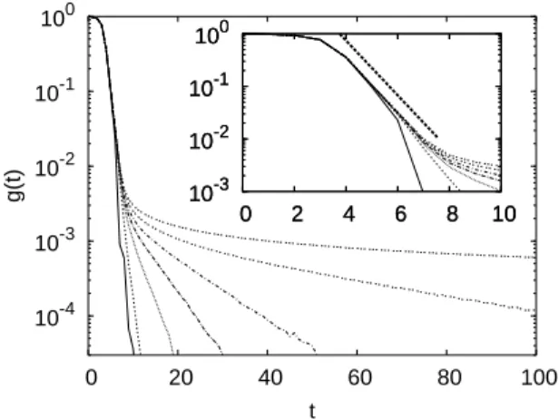
g(t) = (f(t)−f(∞))/(f(0)−f(∞)); (5) in this wayg(t)drops from 1 to 0 whent goes from 0 to∞. We note that f(0) =1 while, for a chaotic system, f(∞)is given by the ratioA0/Ac, withAcbeing the area of the chaotic component to which the initial distribution belongs.
The behavior ofg(t)is shown in Fig. 1, forK0= (
√
10-4 10-3 10-2 10-1 100
0 20 40 60 80 100
g(t)
t 10-3 10-2 10-1 100
0 2 4 6 8 10
10-3 10-2 10-1 100
0 2 4 6 8 10
FIG. 1: Decay of the fidelityg(t)for the sawtooth map with the parametersK0= (
√
5+1)/2 andε=10−3 for different values of L=1,3,5,7,10,20,∞from the fastest to the slowest decaying curve, respectively. The initial phase space density is chosen as the char-acteristic function on the support given by the (q,p)∈[0,2π)×
[−π/100,π/100]. Note that between the Lyapunov decay and the exponential asymptotic decay there is a∝1/√tdecay, as expected from diffusive behavior. Inset: magnification of the same plot for short times, with the corresponding Lyapunov decay indicated as a thick dashed line.
0.1 1
1 10
γ
L
FIG. 2: Asymptotic exponential decay rates of fidelity for the saw-tooth map (K0= (
√
5+1)/2,ε=10−3) as a function ofL. The rates are extracted by fitting the tails of the fidelity decay in the Fig. 1 (tri-angles) and from the discretized Perron-Frobenius operator (circles). The line denotes the∝1/L2behavior of the decay rates, as predicted by the Fokker-Planck equation.
∝1/√Dtuntil the diffusion timetD∼L2/Dand then the as-ymptotic relaxation to equilibrium takes place exponentially, with a decay rateγ(shown in Fig. 2) ruled not by the Lya-punov exponent but by the largest Ruelle-Pollicott resonance [22].
We determine numerically these resonances for the saw-tooth map using the method of Refs. [23, 24], namely by diagonalizing a discretized (coarse-grained) classical propa-gator [19].
In Fig. 2 we illustrate a good agreement between the asymptotic decay rate of fidelity (extracted from the data
10-4 10-3 10-2 10-1 100
1 10 100 1000
g(t)
t
FIG. 3: Decay of fidelity for the stadium billiard with radiusR=1 and length of the straight segmentsd0=2 (the perturbed stadium hasd=d0+ε, withε=2×10⁻³). The initial phase space density was chosen to be a direct product of a characteristic function on a circle in configuration space, the center of which was at (0.5,0.25) as measured from the center of the billiard and its radius was 0.1, while for momenta theδ(|~p| −1)distribution was used. The dashed line represents the expected∝1/tdecay of fidelity.
of Fig. 1) and the decay rate γ as predicted by the gap in the discretized Perron-Frobenius spectrum. We note that in the diffusive regime the classical motion can be described by the Fokker-Planck equation (∂/∂t)R(p,t) = (D/2)(∂2/∂p2)R(p,t), where R(p,t) =R2π
0 dθρ(θ,p,t) and D∝K02is the diffusion coefficient. This gives an asymptotic relaxation rateγ ∝K02/L2, in agreement with the numerical data of Fig. 2. However, the argument based on the gap in the discretized Perron-Frobenius operator has a more general va-lidity, and applies also in situations in which there is exponen-tial relaxation but no diffusion, for example in the sawtooth map withL=1 (see Fig. 2).
We also point out that curves very similar to those plotted in Fig. 1 are obtained in the presence of stochastic noise, e.g. when the backward evolution is driven by a time-dependent kicking strength K(t) =K0+ε(t), with {ε(t)}t=1,2,... uni-formly and randomly distributed inside the interval [−ε,ε]. This means that the effect of a noisy environment on the decay of fidelity for a classically chaotic system is similar to that of a generic static Hamiltonian perturbation.
10-5 10-4 10-3 10-2 10-1 100
1 10 100
g(t), D(2t)
t
FIG. 4: Decay of fidelity for the kicked rotator withK0=2.5,L=1, andε=10−3(full curve). The support of the initial (characteristic) density is(q,p)∈[0,0.2]×[0,0.2]. The dotted curve gives the expo-nential decay determined by the Lyapunov coefficient (about 0.534), while the dashed line shows the∝t−0.55behavior. The decay of cor-relatorDfor the same initial density and for twice the timetis also shown (dot-dashed curve.)
(4) withF0=K0sinθ) in the regime with mixed phase space dynamics (α≈0.55 forK0=2.5,L=1, see Fig. 4).
Finally we remark that the short time Lyapunov decay of fidelity is by no means a typical feature of correlation func-tions. This can be clearly seen in the dot-dashed curve of Fig. 4, which represents the decay of the correlatorD(t) = (C(t)−
C(∞))/(C(0)−C(∞)), withC(t) =RΩd~xρ0(~x,t)ρ(~x,0). Actu-ally the short time decay ofD(t)is determined by the motion of the “center of mass” of the initial distributionρ(~x,0), a triv-ial effect which is suppressed in fidelity due to the backward evolution.
In conclusion, in chaotic systems the asymptotic decay of classical fidelity, exponential or power law, is analogous to the asymptotic decay of correlation functions. It would be inter-esting to understand what are the implications of such connec-tion for the decay of quantum fidelity.
III. STABILITY OF QUANTUM MOTION UNDER SYSTEM’S PERTURBATIONS
In this section we discuss the same question as in the previ-ous one, now in the light of quantum mechanics, namely the stability of quantum motion against system’s perturbation. We define the quantum fidelity in analogy to (1) as
f(t) =|hψε(t)|ψ0(t)i|2 (6) where
|ψε(t)i=Uεt|ψi, |ψ0(t)i=U0t|ψi (7) are perturbed and unperturbed propagators, respectively, gen-erated by the Hamiltonian Hε = H0+εV, namely Uεt = exp(−iHεt/~).
As it is discussed in more detail in contribution [27], the quantum fidelity (6) is expected to follow the classical fidelity
(1) up to the Ehrenfest time, which for a chaotic system with effective Lyapunov exponentλ, reads ast∗=ln(1/~)/(2λ).
Obviously, for times shorter thant∗, the decay of quantum fidelity is determined by classical mechanics. For initial local-ized wave-packets|ψiwe expect initial exponential decay of fidelity with perturbation independent (Lyapunov) exponentλ
fLyap(t) =exp(−λt). (8) For sufficiently strong perturbation strengthε, namelyσ:= ε/~≫1, the quantum fidelity drops to a saturation value f(∞)∼1/N (whereN is the dimension of the Hilbert space, N∼~−danddis the number of degrees of freedom) before the Ehrenfest timet∗is reached. This regime is usually referred to as theLyapunov regimeof fidelity decay and has been first described in Ref. [10].
When the dimensionless parameter σ becomes less than one, σ <1, then one may start to use time-dependent-perturbation theory in order to calculate the fidelity decay. This regime is usually referred to as the Fermi-Golden-Rule regime, and in the case of classically chaotic (mixing) dynam-ics, fidelity decays exponentially
fFGR(t) =exp(−Γt). (9) The exponentΓwhich can be understood also as the width of the Local density of states [12], can be computed [7] in terms of a 2-point time-correlation function of the perturbation C(t) =hVV(t)i − hVi2,V(t) =exp(iH0t/~)Vexp(−iH0t/~), namely as
Γ=ε2D, D:=
Z ∞
−∞dtC(t). (10) In fact, for sufficiently small effective Planck constant~the correlation functionC(t)and diffusion constantDcan be com-puted in terms of classical mechanics. One should note that σ=1 represents a border between classicalσ>1, and quan-tumσ<1 behavior of fidelity [17].
However, this formula (9) works only for times shorter than the Heisenberg timetH=2π~ρwhereρis the density of states. For longer times, quantum correlation functionC(t)starts to be dominated by quantum fluctuations and another approach has to be used. If the perturbationεis so small that a signifi-cant decay of fidelity is taking place after the Heisenberg time tH, then the stationary perturbation theory may be used [13] in order to derive a Gaussian decay of fidelity
fpert(t) =exp(−4ε2Dt2/~2) (11) Comparing the inverse decay rate 1/Γof the formula (9) with the Heisenberg time, we obtain the perturbative border [7, 12, 13]εpert∼~d/2+1orσpert∼~d/2such that forσ<σpert the formula (11) is globally valid.
1e-10 1e-08 1e-06 0.0001 0.01 1
0 500 1000 1500 2000 2500 3000 3500 4000 4500 5000
|F(t)|
2
t
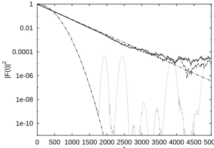
FIG. 5: Fidelity decay for two coupled kicked tops, for perturbation strengthε=8·10−4and for angular momentumJ=200. The upper curves are fork=20 (classically chaotic regime), solid curve for a coherent initial state and dashed curve for a random initial state, and the lower – dotted curve is fork=1 (KAM, quasi-regular regime) with a coherent initial state. The exponential and Gaussian chain curves give, respectively, the expected theoretical decays described by formulae (9) and (12).
decay of dynamical correlations, in a generic (regular) case yields quadratic decay of fidelity in the regime of linear re-sponse, F(t) =1−Cε2t2/~+O(ε4). For initial Gaussian wave-packets one can even show that the global decay in such a case is a simple Gaussian
fregular(t) =exp(−ε2Ct2/~) (12) where the constantCcan be computed solely from the classi-cal data, such as the classiclassi-cal limit of the perturbation observ-ableV and the parameters of initial wave-packet.
Comparing the quantum fidelity decays for chaotic (9) as compared to regular (12) classical mechanics, one finds that the former decays on a time scaletch∼~2ε−2 whereas the latter decays on a time scaletreg∼~1/2ε−1. Therefore, for sufficiently small perturbation ε(for σ≪~1/2) the asymp-totic fidelity decay for classically chaotic dynamics is slower than for classically regular dynamics. (Note that forrandom initial statessuch aparadoxicalbehavior takes place even for σ≪1.) This behavior is not in contrast with the correspon-dence principle as it takes place for time scales beyond the breaking timet∗for quantum classical correspondence. One should always keep in mind the non-commutativity of the lim-its~→0 andε→0.
Let us make a short illustration in terms of a simple numer-ical experiment. We will consider a system with two degrees of freedom, a pair of coupled kicked tops, described by two independent SU(2) variables (angular momenta)J~1and~J2.
A quantum unitary propagator, with some external coupling parameterk, for one-period of the kick reads
U=e−iπ2J1ye−iπ2J2ye−ikJ1zJ2z/J. (13)
The perturbed propagator is obtained by perturbing the para-meterk, so thatUε=U(k+ε). The generator of perturbation
is therefore
V = 1
J2J1zJ2z, (14)
The modulus of angular momentumJ is fixed and equal for both tops, and determines the effective value of Planck con-stant ~=1/J. The total Hilbert space dimension is N = 1/(2J+1)2.
We have chosen two regimes of qualitatively different clas-sical dynamics of the system, namely non-ergodic (KAM) regime fork=1 where the vast majority of classical orbits are stable, and the mixing regime fork=20 where no sig-nificant traces of stable classical orbits. As for initial states we take direct products of SU(2) coherent states centered at two points(ϑ1,2,ϕ1,2) on the two spheres. In Fig. 5 we show the fidelity decay atJ=200 and ε=8·10−4in non-ergodic and mixing cases started from the coherent state with (ϑ1,ϕ1) = (ϑ2,ϕ2) =π(1/
√
3,1/√2). In the most important quantum regime, wheret∗≪t≪tH, we find excellent agree-ment between the theoretical predictions (9) and (12) and the numerics. In the ergodic-mixing regime (k=20) we show for comparison also the fidelity decay for a random initial state which is (due to ergodicity) almost identical to the case of co-herent initial state.
In this section we have shown that the behavior of quan-tum fidelity is, beyond the Ehrenfest time scalet∗, drastically different that for a classical fidelity. In general we may claim that quantum fidelity decays slower than the classical fidelity. Recently, we have discovered even more drastic particular sit-uation, namely the phenomenon of quantum freeze of fidelity [28] which takes place for perturbations wit all diagonal el-ements identically vanishing in the eigenbasis of the unper-turbed Hamiltonian. Such cases can sometimes emerge natu-rally due to symmetry.
IV. CHAOS INDUCED DECOHERENCE
s
a
l
Λ
absorber
screen
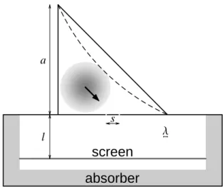
FIG. 6: The geometry of the numerical double-slit experiment. All scales are in proper proportions. The two slits are placed at a distance son the lower side of the billiard
[5]. This fact suggests the complete quantum decoherence in the final steady state for any initial state even though the steady state is formally a pure quantum state. Yet this argument is not completely convincing and a more clear evidence is required. In a recent paper [29] this question has been discussed by considering one of the basic experiments on which rests quantum mechanics, namely a phenomenon which, in the words of Richard Feynmann [30], ”... is impossibleabsolutelyimpossible, to explain in any classical way, and which has in it the heart of quantum mechanics. In reality, it contains the only mystery.” : the double slit experiment.
The following numerical, double-slit experiment has been performed. The time dependent Schr¨odinger equation i~∂
∂tΨ(x,y,t) =HˆΨ(x,y,t), with ˆH = pˆ
2/(2m), has been solved numerically [31] for a quantum particle which moves freely inside the two-dimensional domain as indicated in Fig. 6 (full line). Note that the domain is composed of two regions which are connected only through two narrow slits. We refer to the upper bounded region as to thebilliard do-main, and to the lower one as theradiating region. The scaled units have been used in which Planck’s constant~=1, mass m=1, and the base of the triangular billiard has lengtha=1. The initial stateΨ(t=0)is a Gaussian wave packet (coherent state) centered at a distancea/4 from the lower-left corner of the billiard (in both Cartesian directions) and with velocity~v pointing to the middle between the slits. The screen is at a dis-tancel=0.4 from the base of the triangle. The magnitude of velocityv(in our units equal to the wave-numberk=v) sets the de Broglie wavelengthλ=2π/k. In our experiment we have chosenk=180 corresponding to approximately 1600th excited states of the closed quantum billiard. The slits dis-tance has been set tos=0.1≈3λand the width of the slits isd=λ/4. The wave-packet is also characterized by the po-sition uncertaintyσx=σy=0.24. This was chosen as large
as possible in the present geometry in order to have a small uncertainty in momentumσk=1/(2σx).
The lower, radiating region, should in principle be infinite. Thus, in order to efficiently damp waves at finite boundaries, we have introduced an absorbing layer around the radiating re-gion. More precisely, in the region referred to as absorber, we have added a negative imaginary potential to the Hamiltonian H→H−iV(x,y),V ≥0, which, according to the time de-pendent Schr¨odinger equation, ensures exponential damping in time. In order to minimize any possible reflections from the border of the absorber, we have chosenV to be smooth, starting from zero and then growing quadratically inside the absorber. No significant reflection from the absorber was de-tected and this ensures that the results of our experiment are the same as would be for an infinite radiating region.
While the wave-function evolves with time, a small proba-bility current leaks from the billiard and radiates through the slits. The radiating probability is recorded on a horizontal line y=−lreferred to as the screen. The experiment stops when the probability that the particle remains in the billiard region becomes vanishingly small. We define the intensity at the po-sitionxon the screen as the perpendicular component of the probability current, integrated in time
I(x) =
Z ∞
0 d
tImΨ∗(x,y,t)∂
∂yΨ(x,y,t)|y=−l. (15) By conservation of probability the intensity is normalized,
R∞
−∞dxI(x) =1, and is positiveI(x)≥0. I(x)is interpreted as the probability density for a particle to arrive at the screen positionx. According to the usual double slit experiment with plane waves, the intensity I(x) should display interference fringes when both slits are open, and would be a simple uni-modal distribution when only a single slit is open. This is what we wanted to test with a more realistic, confined geometry. The resulting intensities are shown in Figs. 7, 8(red curves).
0 0.5 1 1.5 2 2.5
-0.8 -0.4 0 0.4 0.8
I(x)
x
I(regular)
I(chaotic) (I1 + I2)/2
FIG. 7: The total intensity after the double-slit experiment as a func-tion of the posifunc-tion on the screen.I(x)is obtained as the perpendicu-lar component of the probability current, integrated in time. The red full curve indicates the case of regular billiard, while the blue dot-ted curve indicates the case of chaotic one. The green dashed curve indicates the averaged intensity over two 1-slit experiments, with ei-ther the regular or chaotic billiard (with results being practically the same, see Fig. 8).
0 0.5 1 1.5 2
-0.8 -0.4 0 0.4 0.8
I(x)
x
I1,I2(regular)
I1,I2(chaotic)
FIG. 8: The two pairs of curves represent the intensities on the screen for the two 1-slit experiments (with either one of the two slits closed). The red full curves indicate the case of the regular billiard while the blue dotted ones indicate the case of chaotic billiard.
pact direction(vx,vy)is always accompanied with a reflected direction(−vx,vy). The pattern on the screen is then a
sym-metricsuperposition of the two interference images, one being a reflection (x→ −x) of the other. In this way one can also un-derstand that the visibility of the interference fringes may vary with the direction of the initial packet.
We also remark that the spacing between interference fringes is in agreement with the usual condition for plane waves that the difference of the distances from the two slits to a given point on the screen is an integer multiple ofλ.
Let us now make a simple modification of our experiment. We replace the hypotenuse of the triangle by the circular
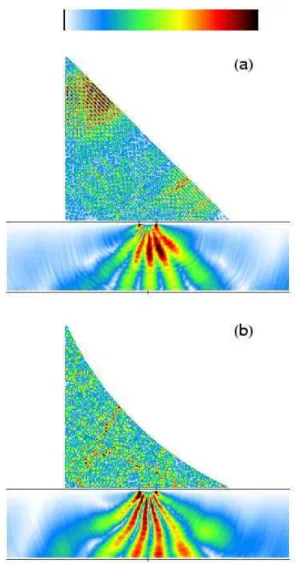
FIG. 9: Typical snapshots of the wave-function (plotted is the prob-ability density) for the two cases: (a) for the regular billiard at t=0.325, and (b) for the chaotic billiard att=0.275 (both cases correspond to about half the Heisenberg time). The probability den-sity is normalized separately in both parts of each plot, namely the probability density, in absolute units, in the radiating region is typi-cally less than 1% of the probability density in the billiard domain. The screen, its center, and the positions of the slits are indicated with thin black lines. Please note that the color code on the top of the figure is proportional to the square root of probability density.
of time, there is a well defined phase relation between the wave function at both slits. Yet, as time proceeds, this phase relation changes, and it is lost after averaging over time. This is nicely illustrated by the snapshots of the wave-functions in the regular and chaotic case shown in Fig. 9. While in the regular case, the jets of probability emerging from the slits always point in the same direction and produce a clear time-integrated fringe structure on the screen, in the chaotic case, the jets are trembling and moving left and right, thus upon time-integration they produce no fringes on the screen [33].
The results of this numerical experiment can be under-stood in terms of fast decay of spatial correlations of eigenfunctions of chaotic systems. In the limit of small slits opening d ≪λ, the intensity on the screen, according to simple perturbation expansion in the small parameter d/λ, can be written as
I(x) =I1(x) +I2(x) +C(s)f(x), (16) where f(x)is some oscillatory function determining the pe-riod of the fringes, andC(s)is the spatial correlation func-tion of the normal derivative of the eigenfuncfunc-tions Ψn of the closed billiard at the positions (−s/2,0) and (s/2,0) of the slits, written in the Cartesian frame with origin in the middle point between the slits. In particular, C(s) = α ∑n|cn|2∂yΨn(−s/2,0)∂yΨn(s/2,0), wherecnare the expan-sion coefficients of the initial wave-packet in the eigenstates Ψn, and α is a constant such thatC(0) =1. Note that this eigenstate correlation functionC(s), which also depends on the initial state through the expansion coefficients cn, is di-rectly proportional to the visibility of the fringes. One may use well knownrandom plane wave model for chaotic billiards [32], in combination with a method of images to account for the boundary condition, to show that quantum chaotic eigen-states exhibit decaying correlations withC(s) =J1(ks)/(ks) whereJ1is a first order Bessel function, whereas for regu-lar systemsC(s)typically does not decay (but oscillates) so it produces interference fringes. In our case of half-square
billiard we find, for large k, C(s) =e−σ2ks2/2(k2
xcos(kys) +
ky2cos(kxs))/k2. The Gaussian prefactor can easily be under-stood, namely there is no interference if the size of the wave-packet is smaller than the slit-distance, or equivalently, if un-certainty in momentumσkis much larger than 1/s.
Disappearance of interference fringes can be directly re-lated to decoherence. If A is a binary observable A ∈
{1,2}which determines through which slit the particle went, thenC(s)is proportional to the non-diagonal matrix element
h1|ρ|2iof the density matrix in the eigenbasis ofA, and is thus a direct indicator of decoherence.
The result presented here provides therefore, from one hand, a vivid and fundamental illustration of the manifesta-tions of classical chaos in quantum mechanics. On the other hand it shows that, by considering a pure quantum state, in absence of any external decoherence mechanism, internal dy-namical chaos can provide the required randomization to en-sure quantum to classical transition in the semiclassical re-gion. The effect described in this letter should be observable in a real laboratory experiment.
V. CONCLUSIONS
In this paper we have presented two different, general il-lustrations of observable effects of quantum chaos. On one hand, we have shown that sensitivity to system’s perturbations is clearly connected with the nature of the underlying classical dynamics. The concepts of classical and quantum Loschmidt echoes are relatively new but may have important implications in statistical physics and in the field of quantum information and quantum computation. On the other hand, we have shown that quantum chaos can act also as a source of noise thus pro-ducing effects equivalent to decoherence, such as destroying interference fringes in a double slit experiment.
The work has been financially supported in part by the grant DAAD19-02-1-0086, ARO United States, and by the grant (T.P.) P1-0044 of the Ministry of Science, Education and Sports of Republic of Slovenia.
[1] F. Haake,Quantum Signatures of Chaos, 2nd edition (Springer-Verlag, Heidelberg, 2001).
[2] H.-J. St¨ockmann, Quantum Chaos - An Introduction (Cam-bridge University Press, Cam(Cam-bridge, 1999).
[3] I.P. Cornfeld, S.V. Fomin and Y.G. Sinai, Ergodic theory (Springer-Verlag, 1982).
[4] G. Casati, B. V. Chirikov, I. Guarneri and D. L. Shepelyansky, Phys. Rev. Lett.56, 2437 (1986).
[5] G. Casati and B. V. Chirikov, in: “Quantum chaos: between order and disorder” (Cambridge University Press, Cambridge, England, 1995) p.3; G. Casati and B. V. Chirikov,PhysicaD86, 220 (1995); G. Casati and B. V. Chirikov,Phys. Rev. Lett.75, 350 (1995).
[6] A. Peres, Phys. Rev. A30, 1610 (1984).
[7] T. Prosen and M. ˇZnidariˇc, J. Phys. A35, 1455 (2002); T. Prosen, Phys. Rev. E65, 036208 (2002).
[8] G. Benenti, G. Casati and G. Strini, Principles of Quantum Computation and Information, Vol. I:Basic concepts(World Scientific, Singapore, 2004).
[9] M.A. Nielsen and I.L. Chuang, Quantum Computation and Quantum Information (Cambridge University Press, Cam-bridge, 2000).
[10] R.A. Jalabert and H.M. Pastawski, Phys. Rev. Lett,86, 2490 (2001).
[11] F.M. Cucchietti, H.M. Pastawski and D.A. Wisniacki, Phys. Rev. E65, 045206(R) (2002).
[12] Ph. Jacquod, P.G. Silvestrov and C.W.J. Beenakker, Phys. Rev. E64, 055203(R) (2001),
[13] N.R. Cerruti and S. Tomsovic, Phys. Rev. Lett. 88, 054103 (2002).
[15] Z.P. Karkuszewski, C. Jarzynski and W.H. Zurek, quant-ph/0111002.
[16] D.A. Wisniacki and D. Cohen, quant-ph/0111125. [17] G. Benenti and G. Casati, Phys. Rev. E65, 066205 (2002). [18] J. Vanicek and E. J. Heller, Phys. Rev. E68, 056208 (2003). [19] G. Benenti, G. Casati and G. Veble, Phys. Rev. E67, 055202(R)
(2003).
[20] B. Eckhardt, J. Phys. A: Math. Gen.36, 371 (2003). [21] G. Veble and T. Prosen, Phys.Rev.Lett.92, 034101 (2004). [22] D. Ruelle, Phys. Rev. Lett.56, 405 (1986).
[23] J. Weber, F. Haake and P. ˇSeba, Phys. Rev. Lett. 85, 3620 (2000).
[24] M. Khodas, S. Fishman and O. Agam, Phys. Rev. E62, 4769 (2000).
[25] F. Vivaldi, G. Casati and I. Guarneri, Phys. Rev. Lett.51, 727 (1983).
[26] C. F. F. Karney, Physica 8D, 360 (1983); B.V. Chirikov and D.L. Shepelyansky, Physica13D, 395 (1984).
[27] T. Prosen and M. ˇZnidariˇc, Braz. J. Phys. (2005), this volume. [28] T. Prosen and M. ˇZnidariˇc, New J. of Phys.109(2003); Phys.
Rev. Lett. (2005),in press.
[29] G. Casati and T. Prosen, “Quantum chaos and the double-slit experiment”,nlin.CD/0403038 .
[30] R. P. Feynman, Lecture Notes in Physics, Vol. 3
(Addison-Wesley, 1965), p.1-1.
[31] We have implemented an explicit finite difference numeri-cal method withλ/h≈12 mesh points per de Broglie wave-lengthλ wherehis the step-size of the spatial discretization. The stability of the method was enforced by using unitary power-law expansion of the propagator, namely Ψ(t+τ) =
∑nj=0 1
n!(− iτ
~Hˆ)jΨ(t) where ˆH=− ~2
2m∆ and ∆ is a discrete
Laplacian. Using temporal step-sizeτ=h2, the required ordern to obtain numerical convergence within machine precision was typically small,n<10. The implementation of the finite dif-ference scheme was straightforward for the triangular geome-try, since the boundary conditions conform nicely to the dis-cretized Cartesian grid. For the case of chaotic billiard, we used a unique smooth transformation(x,y)→(x,f(y))which maps the chaotic billiard geometry to the regular one, and slightly modifies the calculation of the discrete Laplacian without alter-ing its accuracy (due to smoothness off(y)).
[32] M. V. Berry, J. Phys. A: Math. Gen.10, 2083 (1977).