Braz. J. Phys. vol.34 número4A

(1)

Neutrinos at 1%: A Reactor Based Measurement of

θ

₁₃

David Reyna

Argonne National Laboratory 9700 S. Cass Avenue, Argonne, IL 60439, USA

Received on 2 December, 2003

Past studies of neutrinos and the recent results on neutrino mixing have opened up many new possibilities as well as the understanding that neutrino mixing is very different from the better known quark mixing. The last remaining unmeasured component of the neutrino mixing matrix (Ue3) also provides a window to understanding

neutrino matter effects, the mass hierarchy, and the possibility of measuring leptonic CP violation. A discussion of the benefits and difficulties of pursuing such a measurement with reactor neutrinos will be presented. In addition, possible sites for such an experiment will be discussed, including a location in Brazil.

1 Introduction to Flavor Mixing

The process of flavor oscillation arises from the fact that the flavor eigenstates and the mass eigenstates appear not to be the same. By considering the flavor and mass states to be rotated with respect to each other by an angleθ, one can de-compose a neutrino flavor state into a linear combinations of mass states (νi). In the case of only 2 eigenstates, this is

represented as

νe = ν1cosθ+ν2sinθ (1) νµ = −ν1sinθ+ν2cosθ. (2) We are familiar with this rotation of bases in the quark sector where an analog to the equations above were the ori-gin of Cabibbo Mixing[1] between d and s quarks resulting in the 2-by-2 mixing matrix

d′

s′

=

cosθc sinθc

−sinθc cosθc

d s

. (3)

This formalism has been further extended to include 3 fla-vor mixing by Kobayashi and Maskawa[2]. The 3-by-3 mi-xing matrix is usually referred to as the Cabibbo-Kobayashi-Maskawa (CKM) matrix



 d′

s′

b′



=





Vud Vus Vub

Vcd Vcs Vcb

Vtd Vts Vtb



 

 d s b



. (4)

Over the last decade, much experimental effort has gone into measuring the individual elements of the CKM matrix. To very high precision, the values show that the diagonal ele-ments are very close to 1 while the off-diagonal eleele-ments are very close to zero. The implication of this is that the flavor basis and the mass basis are very nearly identical.

In the neutrino sector, a similar 3-by-3 mixing matrix has been constructed. This is usually referred to as the MNS[3] matrix:



 νe

νµ

ντ



= 



Ue1 Ue2 Ue3 Uµ1 Uµ2 Uµ3 Uτ1 Uτ2 Uτ3



 

 ν1 ν2 ν3



. (5)

While the age of neutrino oscillation measurements is cur-rently very young, all of the elements of the MNS mixing matrix have been coarsely extracted from current measure-ments to about 30-40% precision. The current mean values are

|Umean|=





0.8 0.57 0.0 0.45 0.5 0.7 0.34 0.6 0.68



. (6)

Notice that the structure of this matrix differs greatly from the CKM matrix which was primarily diagonal. In the MNS matrix, all elements, with the exception ofUe3, appear to be

of order unity. Thus, contrary to the quark sector in which the flavor and mass bases were nearly identical, the neutrino flavor and mass bases are very nearly orthogonal.

2 The Significance of

U

_e₃

On examination of the experimentally determined values of the MNS matrix in Eq. 6, one quickly notices that the value forUe3is far different from all the other elements. The cur-rent best limits from experiment provide an upper bound of |Ue3|<0.22. To understand better the significance of this, we can look at the Chau-Keung[4] parameterization of the MNS matrix in which the matrix is broken down into 2-by-2 rotational matrices through three Euler angles with a single imaginary phase. Using the anglesθijto refer to the mixing

(2)

UM N S = U23U13U12 (7)

=





1 0 0

0 c23 s23

0 −s23 c23 

 



c13 0 s13eiδ

0 1 0

−s13e−iδ 0 c13 

 



c12 s12 0 −s12 c12 0

0 0 1



 (8)

=





c13c12 c13s12 s13eiδ

−s12c23−c12s23s13e−iδ c12c23−s12s23s13e−iδ s23c13 s12s23−c12c23s13e−iδ −c12s23−s12c23s13e−iδ c23c13



. (9)

⌈

We can first conclude that θ13 is small since U_e3 =

sinθ13eiδ. Perhaps more interesting, however, is that the imaginary phaseδ, which would be responsible for CP vio-lation in the lepton sector, is also present. In fact, any physi-cal process for which this leptonic CP violating term would be present also contains the multiplicative factor ofsinθ13. Thus a non-zero value ofθ13is required for any leptonic CP violation to be observed. Recognition of this fact has focu-sed significant attention on our ability to measure a non-zero value ofθ13through neutrino oscillation measurements.

3 Neutrino Oscillation

If we return briefly to Eqs. 1 and 2, in which the flavor states were expressed as a linear combination of the mass states, and express the propagation of a neutrino in time as ν(t) = e−iEt_ν₍₀₎_{. Then, beginning with a pure neutrino}

flavor state (νe), the probability of finding a second neutrino

flavor (νµ) is just

⌋

P(νe→νµ) =νµ(0)|νe(t) = sin

2 θcos2

θ

e−iE2t−e−iE1t 2

(10)

= sin2

(2θ) sin2

1.27∆m2L E

. (11)

⌈

Equation 11 is the standard oscillation equation for any two neutrino mixing. The parameterθis referred to as the mixing angle and the factorsin2

(2θ)is merely the amplitude of the oscillation. A value of zero forsin2

(2θ)would imply that no oscillations would occur. The second factor defines the oscillation itself. The frequency of the oscillation is go-verned by the difference between the squared masses of the two mass states: ∆m2

12 = m

2 1−m

2 2 (eV

2

). The propa-gation of the oscillation is dependent on L/E where L is the distance from the source to the detector in kilometers and E is the energy of the neutrino in GeV.

The current best results from experiments (primarily Super-Kamiokande and SNO) have established two ∆m2 values relating to the two primary oscillations which have been observed: the solar neutrino deficit (νedisappearance)

∆m2

solar ≃5×10−

5 eV2

and the atmospheric neutrino de-ficit (νµ disappearance)∆m2atm ≃2×10−

3 eV2

. It is im-portant to note that in the standard neutrino picture with 3 neutrino flavors, there are only two independent mass dif-ferences since the third can be related to the other two by

∆m2

13 = ∆m 2

12+ ∆m 2

23. There is evidence from LSND which suggests an additional much larger∆m2

> 0.1eV2

for the processν¯µ → ν¯e. However, since this is not

con-firmed by the KARMEN[5] experiment and would require new physics which has not been observed, it will not be con-sidered for this discussion. It is usually accepted notation to refer to the smaller mass difference as being between mass statesν1 andν2, thus ∆m

2

12 ≡ ∆m 2

solar. However, it is

important to realize that there exists no evidence yet to esta-blish the hierarchy of the mass states. Therefore, we do not know if the masses of the two close mass states (ν1andν2) are lower (normal hierarchy) or higher (inverted hierarchy) thanν3.

(3)

⌋

P(νe→νe) = 1−cos

4

(θ13) sin 2

(2θ12) sin 2

1.27∆m2 12

L E

−sin2

(2θ13) sin 2

1.27∆m2

atm

L E

. (12)

⌈

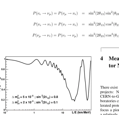
This equation is plotted in Fig. 1 as a function of L/E. One can easily see that the two oscillation frequencies are well separated. What is also apparent, however, is the significant affect of the different mixing angles on the amplitudes of the oscillation. To be able to properly understand the magnitude

of the oscillations, one must account for all three mixing angles. The following equations show various flavor oscil-lation transitions under full three flavor mixing (excluding CP violation), but restricted to only the large∆m2

atm:

⌋

P(νe→νµ) =P(νµ→νe) = sin

2

(2θ13) sin 2

(θ23) sin 2

1.27∆m2

atm

L E

(13)

P(νe→ντ) =P(ντ →νe) = sin

2

(2θ13) cos 2

(θ23) sin 2

1.27∆m2

atm

L E

(14)

P(νµ→ντ) =P(ντ→νµ) = sin

2

(2θ23) cos 4

(θ13) sin 2

1.27∆m2

atm

L E

(15)

⌈

10-1 1 10

0 0.2 0.4 0.6 0.8 1

L/E (km/MeV) )_e

ν

→

e

ν

P(

) = 0.8

12

θ

(2

2

; sin

-5

= 5 x 10

21 2

m

∆

) = 0.1

13

θ

(2

2

; sin

-3

= 2 x 10

31 2

m

∆

Figure 1. The survival probability ofνe¯ _{as a function of L/E. This} is a graphical representation of Eq. 12 where the values for the mixing angles and mass differences are set to the current best evi-dence from experimental results. The value ofsin2

(2θ13)is chosen

to be the maximum allowed by the current exclusion limit.

4 Measurement of

θ

₁₃

_with

Accelera-tor Neutrinos

There exist several current accelerator based neutrino beam projects: NuMI/MINOS at Fermilab, K2K in Japan, and CERN-to-Gran Sasso (CNGS). The accelerators at these la-boratories create a neutrino beam by colliding intense acce-lerated proton beams with a fixed dense target to create and focus a pion beam which decays in flight. This results in a relatively pureνµ beam of a few GeV which can then be

detected at distances up to 1000km away by detectors with sufficient mass. The current set of accelerator based experi-ments are primarily looking forνµdisappearance at the first

oscillation maximum of the atmospheric∆m2

. Thus from Eqs. 15 and 13 we can simply write this as

⌋

P(νµ→νµ) = 1−

sin2

(2θ23) cos 4

(θ13) + sin 2

(2θ13) sin 2

(θ23) sin 2

1.27∆m2

atm

L E

. (16)

⌈

Unfortunately, given our current knowledge of the mi-xing angles, the first amplitude term will dominate:

sin2

(2θ23) cos 4

(θ13) ∼ 1 while sin 2

(2θ13) sin 2

(θ23) <

0.05. This means that extracting the value forsin2

(2θ13) from this process will be extremely difficult.

However, by recalling thatsin2

(θ23)∼1and looking at Eq. 13, we note that if a future experiment could isolate the exclusive processνµ →νe, the amplitude of any measured

oscillation would directly yield the magnitude ofsin2

(4)

This is the intent of the two proposed future long baseline projects NuMI/Off-Axis and JPARC-SK. These experiments are designed to look for neutrino interactions with an elec-tron in the final state, as opposed to a muon, from an accele-rator basedνµbeam at the optimal L/E for the atmospheric

∆m2

. This measurement will be complicated by the fact that several background sources exist. The standard accele-rator based neutrino beam contains a small (∼1%) contami-nation ofνedue to decays of kaons and muons off the

pro-ton target. There are also small contributions of final state electrons fromντinteractions in which a highly energeticτ

decays viaτ→e−_ν_¯

eντ. In addition, depending on the

gra-nularity of the detector, there are many processes which can produce showers which look very similar to electron signa-tures (e.g.νN →νN π0

whereπ0 →γγ).

While such backgrounds may make measuring a small oscillation effect difficult, they are by no means impossible to measure or control. However, when one includes the pos-sible effects of leptonic CP violation or matter effects, the ability to extract a value forsin2(2θ13)becomes significan-tly more difficult. This subject is explored in much more detail in [6] and others. For the purposes of this discussion, it is sufficient to say that all three of these effects (flavor os-cillation, CP violation, and matter effects) can enhance or diminish an observedνµ → νe signal. This results in an

eight-fold ambiguity in the extraction ofsin2

(2θ13)from a single long baseline measurement ofP(νµ→νe).

In order to resolve these degeneracies, one would have to make use of the various different dependences on flavor, energy and baseline. Clearly matter effects will be most strongly dependent on the length of the baseline, but detec-tors for these experiments are large (∼50 ktons) so moving them is impossible. Matter effects will also have opposing effects on neutrinos and anti-neutrinos so measurements of bothP(νµ → νe)andP(¯νµ → ν¯e)at a single experiment

would provide useful information. However, CP violation also provides an energy dependent separation between the two oscillation probabilities depending on the actual value of the complex phaseδ. Thus any real attempt to comple-tely resolve these degeneracies would most likely require at least 2 experiments which are running at different energies and baseline distances. In addition, each experiment would likely have to measure both observablesP(νµ → νe)and

P(¯νµ→¯νe).

This presents a long and expensive future program. Gi-ven the required detector sizes and required granularity to detect electron signals, these future accelerator based expe-riments are expected to cost∼$200 million or more. In addi-tion, the construction of these detectors takes 5-10 years and each one of the oscillation measurements would probably require at least 3-5 years worth of running time. However, θ13 could be zero, or small enough that no oscillation sig-nals would be detected, in which case degeneracies would no longer be a concern.

5 Measurement of

θ

₁₃

_{with Reactor}

Neutrinos

Recently, a lot of discussion has focused on the possible al-ternative of measuringθ13with neutrinos from nuclear re-actors. Nuclear reactors provide an isotropic source of pure electron anti-neutrinos (ν¯e). There is a long history of

neu-trino experiments associated with reactors. Some of them have indeed been searches for evidence of neutrino oscil-lation by looking for disappearance effects. In the absence of matter effects, the survival probability of electron anti-neutrinosP(¯νe→ν¯e)is governed by the same equation as

electron neutrinos (Eq. 12). It was pointed out previously in Fig. 1 that a judicious choice of L/E could isolate the effects of one or the other of the∆m2

oscillations. Thus, by staying at small L/E (i.e.ignoring the small∆m2

12) Eq. 12 reduces to

P(¯νe→¯νe) = 1−sin

2

(2θ13) sin 2

1.27∆m2

atm

L E

.

(17) Any observed deficit in neutrino flux would be a direct me-asurement ofθ13. In addition, any such measurement would not suffer from the ambiguities which are seen in accelerator measurements. Neutrinos generated in nuclear reactors are at very low energy and are only detectable in the range 1-10 MeV. The optimal baseline for the first oscillation is there-fore in the range of 1-4 km, depending on the exact value of

∆m2

atm. This distance is much too short for any matter

ef-fects to begin. In addition, disappearance processes are not affected by CP violation without a corresponding violation of CPT . Therefore, any measurement ofθ13 from reactor neutrinos would be clean and unambiguous.

One should not mistake this to imply that such a me-asurement would be easy. In fact, until the recent results from KamLAND[7] which detected effects of the∆m2

12 os-cillation at an average baseline of 180km, no reactor neu-trino experiment had been able to detect signs of oscil-lations. The current world’s limit on sin2

(2θ13) comes from the CHOOZ reactor experiment (sin2

(2θ13) <0.2at

∆m2

atm = 0.002)[8]. This measurement was limited by a

systematic error of about 3% relating to the uncertainty in the reactor power.

Fundamentally, all reactor neutrino experiments have used a similar design. A single detector, placed at a given baseline distance from the reactor core, is used to measure the absolute flux and energy spectrum ofν¯e. This spectrum

is then compared to the theoretically predicted flux and spec-trum based on the reactor’s operating power and the radioac-tive decay of the reactor’s fuel components. Given that the reactor fuel composition changes over time as it is consumed and that the radioactive decay spectra of the individual com-ponents are known to finite precision, the predicted flux and energy spectrum can not be determined to better than 2-3%. Any next generation measurement ofsin2

(5)

90% confidence limit ofsin2(2θ13)<0.02or perhaps a3σ measurement ifsin2(2θ13)>0.05. Making such a measu-rement will require finding a way to limit the systematics to the order of 1%. A method for doing this is discussed in the next section.

6 Experimental Design

An international working group, with members from Eu-rope, North America, Russia and Japan, has been discus-sing methods to make a higher precision measurement of

sin2

(2θ13)using reactor neutrinos. As conceived, the un-certainty in reactor flux and spectrum could be avoided by simultaneously measuring neutrinos from a reactor at two identical detectors which are placed at different baseline dis-tances. The ratio of these two measurements would then be independent of any uncertainties in the source. Ideally, one detector would be placed as close to the reactor as possible to maximize the total neutrino flux and minimize any os-cillation, while the second detector would be placed at the first oscillation maximum. By comparing the ratio of the measured fluxes to the expected fall off (∝ 1/L2

) a non-zerosin2

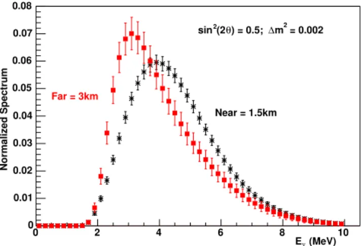
(2θ13)could be detected. In addition, if enough statistics are present, relative spectral distortions could be detected. An example of two such measured energy spectra is shown in Fig. 2.

0 2 4 6 8 10

0 0.01 0.02 0.03 0.04 0.05 0.06 0.07 0.08

= 0.002 2 m ∆ ) = 0.5; θ (2 2 sin

Near = 1.5km Far = 3km

(MeV)

ν

E

Normalized Spectrum

Figure 2. Comparison of the expected measured neutrino energy spectra at baseline distances of 1.5 and 3 kilometers. Oscillati-ons as defined in Eq. 17 are assumed with the parameters set to

∆m2

= 0.₀₀₂_and_sin2

(2θ13) = 0.5(which is 2 and a half times

the current limit in order to magnify the effect). Each shown spec-trum is normalized to the total number of events at that location and the error bars represent the statistical uncertainty for a luminosity of 600 GW-ton-years at the specified baseline distance.

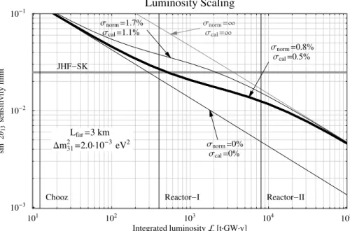
In fact, an interesting observation has been made by M. Lindner et al. [9]. They have pointed out that the com-parison of spectral shapes between the two detectors will have even less dependence on systematic effects than the to-tal flux ratio. Thus for high enough statistics, the spectral shape measurement can actually achieve almost two orders

of magnitude improvement insin2(2θ13)sensitivity. This is demonstrated in Fig. 3 where systematic errors have been classified into two categories: those which relate to ove-rall normalization between the detectors (σnorm) and those

which are uncorrelated bin-to-bin (σcal). One can see that

as total luminosity increases, the sensitivity improves direc-tly with statistics until about 2-400 GW-ton-years at which point the systematics begin to restrict the total flux ratio. However, after 3000 GW-ton-years, the energy spectra com-parison has finally gained enough statistics to allow the me-asurement to be insensitive to σnorm. The ultimate

sen-sitivity is heavily dependent on the choice of the uncorre-lated bin-to-bin systematic error. The value chosen here (σcal= 0.5%) appears reasonable.

One can wonder if the systematic error for the relative normalization between the detectors (σnorm = 0.8%) was

reasonably chosen in the above analysis. It is possible to make an estimate of what is attainable by looking at the re-sults of the Bugey experiment[10] which actually had three detectors. The Bugey detectors were located at very short distances (15m, 40m and 95m) and therefore are not relevant to the atmospheric∆m2

. However, they did attempt a com-parative measurement between their 15m and 40m detectors. In Table I, the systematic errors for a single detector measu-rement (Absolute Normalization) and for the two detector comparative measurement (Relative Normalization) are lis-ted.

The absolute systematics are consistent with other simi-lar reactor measurements. When looking at the systematic errors in the relative measurement, one notes that these are dominated by neutron and positron detection efficiencies. It is important to realize that Bugey used segmented detectors constructed out of stacked rectangular tubes containing li-quid scintillator. The neutron detection efficiency was due mainly to losing neutrons down the gaps between the rectan-gular tubes. The positron detection efficiency was similarly dominated by interactions with the walls of the rectangu-lar tubes. Thus, by avoiding segmented detectors and using a monolithic design as in the case of CHOOZ and Kam-LAND, these errors can reasonably be reduced (the CHOOZ experiment lists an overall detection efficiency of 1.5% for a single detector measurement). The systematic error on the solid angle refers to the fact that the detectors were at such short baselines that the dimension of the reactor core was visible in the angular distribution of the detected neutrino events. Given the small size of these detectors, many events were lost out the sides of the detectors. This provided a dif-ference between the two detectors because of the differing baselines. However, the much larger distances involved in any future two detector measurement (minimum 200m for a near detector) and the much larger detector sizes imply that any such angular based systematics should be negligible.

(6)

101 ₁₀2 ₁₀3 ₁₀4

105 Integrated luminosityt_GW_y

103 102 101

sin

2 2

Θ13

sensitivity

limit

Luminosity Scaling

JHF_SK

Σ_norm_1.7%

Σ_cal_1.1%

Σ_norm_0.8%

Σ_cal_0.5%

Σ_norm_0%

Σ_cal_0%

Chooz Reactor_I _Reactor_II

Σ_norm

Σ_cal

Lfar3 km

_m

31

2 _2.0₁₀3_eV2

Figure 3. The sensitivity to sin2

2θ13 at 90% CL as a function of the integrated luminosity. This plot is taken from [9] and shows the

effect of different values of the normalization errorσnorm and the energy calibration errorσcal. The oscillation was assumed to have

∆m231= 2×10−

3

eV2and the far detector was placed at 3 kilometers from the source.

TABLE I. Breakdown of systematic errors from the Bugey experiment[10]. The absolute normalization refers to the percentage errors when a single detector measurement was made. The relative normalization refers to those errors which remained when a comparison of two detectors was made.

Error Source Absolute Relative

Normalization (%) Normalization (%)

Neutrino Flux 2.8

-νP Cross Section 0.2

-Solid Angle 0.5 0.5

Target Protons 1.9 0.6

Neutron Detection 3.2 1.5

Positron Detection 0.9 0.9

Selection Correlation 1.0

-Signal/Background 25@15m 2.2@40m 0.7@95m

Total 5.0 2.0

Bugey was able to achieve a total relative error of 2%, it seems reasonable to presume that an overall systematic er-ror of less than 1% in a two detector measurement can be achieved.

7 Requirements for an Experimental

Site

As was observed in Fig. 3, one of the most critical factors in the sensitivity tosin2

(2θ13)is overall luminosity. This is a product of the power of the reactor (GW), the mass of the detectors (tons) and the length of time for the experiment (years). To a certain extent, these three components can be

played against each other. However, given that both length of time and detector size require money, it is useful to ma-ximize the reactor power if possible. Most modern reactors produce between 3-4GWthof power per core. Many reactor

facilities have two or three cores on a single site. There is a trade-off in the additional luminosity, however. Each re-actor shuts down periodically to replenish fuel. At a single reactor facility, this provides an opportunity to measure the non-reactor based backgrounds. However, at a multiple re-actor facility, companies tend to avoid having all rere-actors off simultaneously. Thus the backgrounds must be extrapolated from the reduced flux running, introducing an additional er-ror source into the measurement.

(7)

muons. While external vetoes can be constructed to remove these signals from the data stream, the overall rate at the surface is prohibitive. Therefore, any detector must be pla-ced under a significant overburden. In order to keep any background corrections small, and by extension their con-tribution to the systematic errors small, the background rate at the far detector needs to be less than 1%. This implies an overburden of at least 300m of water equivalent (mwe). Further consideration of backgrounds from muon induced production of radioactive isotopes which can produce corre-lated events mimicking the neutrino signal (such as8

He,9 Li and11

Li) have suggested that a larger overburden, perhaps as much as 500 mwe, may be required.

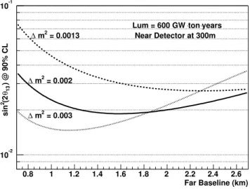
To achieve these levels of overburden, extensive exca-vations may be required. Any reactor facility under consi-deration must have geological conditions that are conducive to such a construction effort. This means that the ground underneath must be stable enough to support boring shafts 200m down and building caverns, or there need to be sur-rounding hills which are high enough and can support ho-rizontally excavated tunnels. The latter possibility is gene-rally preferred since the costs of tunneling into a hillside are expected to be less than for boring a shaft. However, that requires that hills exist at the optimal distance for the oscil-lation measurement. Fig. 4 shows a calcuoscil-lation of sensitivity tosin2

(2θ13)as a function of baseline distance for 3 diffe-rent values of∆m2

atm.

0.8 1 1.2 1.4 1.6 1.8 2 2.2 2.4 2.6 10-2

10-1

= 0.0013

2

m

∆

= 0.002

2

m

∆

= 0.003

2

m

∆

Near Detector at 300m years

⋅

ton

⋅

Lum = 600 GW

Far Baseline (km)

) @ 90% CL

13

θ

(2

2

sin

Figure 4. Statistical sensitivity tosin2

(2θ13)as a function of

base-line distance to the far detector. The statistical power is calculated for a luminosity of 600 GW-ton-years and a 1% systematic limit bin-to-bin. Curves are shown for three values of∆m2

represen-ting the best fit and the upper and lower limits of the 90% allowed region from the Super-Kamiokande experiment.

One can see that for the current best fit of Super-Kamiokande (∆m2

atm = 0.002), the optimal baseline

dis-tance for the far detector is about 1.6km. However, the de-pendence is relatively flat and any location between 1.3km and 2km would provide reasonable sensitivity while main-taining flexibility to various values of∆m2

.

In addition to the usual nuclear reactor facilities in the U.S. and France, locations as diverse as Siberia, Japan, and

Taiwan have been considered for this experiment. Each of these has different advantages. Many have shown distinct difficulties either in finding adequate detector locations, or more commonly, in finding adequate communication and access from the nuclear reactor facility itself. In the next section, we will discuss one very promising reactor facility located at Angra dos Reis, Brazil.

8 An Experiment at Angra dos Reis

Angra dos Reis is located about 150km south of Rio de Ja-neiro. The nuclear facility contains two operational reactors. The Angra-I reactor is an older low power (about 1.5 GWth)

reactor that is not frequently operated. The Angra-II reactor, on the other hand, was brought on-line in 2000 and is con-sistently operated at about 4.1 GWth. The reactors are

loca-ted on the coast and the reactor company controls a strip of land that stretches inland about 1-1.5km and is approxima-tely 4 or 5 km along the coast. All experimental constructi-ons which will be cconstructi-onsidered here would be situated within the reactor company’s site boundaries.

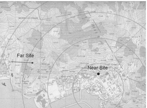
Much of this terrain is mountainous granite with mul-tiple peaks in the 200-600m region. This allows good background reduction to be achieved for an experimental hall with relatively cheap civil construction by tunneling si-deways into such a mountain. Also within the site bounda-ries there exists a town, Praia Brava, which houses most of the 2 or 3 thousand people who work at the reactor facility and also contains a hotel and stores. Such already existing infrastructure could make using this facility more attractive. The company which runs Angra is state owned and ope-rated. One of the unique features of attempting this expe-riment in Brazil is that the presidents of both the electric power company and it’s daughter nuclear power company are former particle physicists who used to do experiments at CERN. As a result, they are very receptive to communicati-ons from members of the Brazilian physics community and have been very helpful in providing resources and access to the facility. A one day site visit has already been performed to evaluate the viability of performing the experiment there. Significant assistance was provided by the director of opera-tions from the reactor facility and we spent significant time with the director of civil construction on the site. With their help, we were able to explore all the possible experimental site locations and arrive at a solution which was acceptable to both the reactor facility and the experimental needs. The reactor company has agreed to supply full detailed cost esti-mates of any civil construction plan that we provide by using their detailed knowledge of the site geology and known con-tractors.

(8)

Figure 5. A topographic map of the nuclear reactor site at Angra dos Reis. The concentric circles are at 500 meter radial intervals from the core of Angra-II. Proposed locations for the near and far detector experimental halls as well as the far detector access tunnel are shown.

western edge of the hillside. This location is easily accessi-ble from the town of Praia Brava and would be very near to the current location of their sewage treatment plant.

It is envisaged to place identical 50 ton fiducial detec-tors at each location. Exact detector designs have not yet been developed, but it is currently assumed that such detec-tors would build off of the developments from other groups. Most likely a 3 volume detector would be optimal: a cen-tral liquid scintillator volume that would be doped with ga-dolinium (target); a surrounding volume of liquid scintilla-tor without gadolinium (gamma catcher); a non-scintillating buffer to shield the radioactivity of the photo-tubes which would be installed at the outer edge of this volume. An ac-tive muon shield would then be required to surround this system. A spherical detector with an active target of 50 tons would have a total diameter of approximately 7.3 meters. The access tunnels and experimental halls have been desig-ned to accommodate these dimensions.

Preliminary estimations have been performed of the sig-nal and background rates for the given detector configura-tion. The detector at the far location is expected to receive about 120 signal events per day, while the near site would be expected to receive about 3000. Some very preliminary background estimations suggest that the far detector would expect less than 10 Hz uncorrelated backgrounds which would easily be vetoed by an active muon shield and about 1-2 correlated background events per day from muon indu-ced radioactive isotopes. Similarly the near detector would expect an uncorrelated background rate of about 830Hz (yi-elding an active live time of 63% after muon vetoing) and a correlated background of approximately 150 events per day. Having a signal to noise rate of about 100 in the far detector and 20 in the near detector should allow

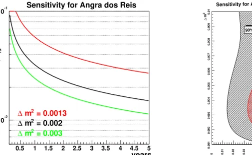
reasona-ble background rejection while maintaining statistical sensi-tivity. Fig. 6 (left) shows the expected statistical sensitivity as a function of time, for the best fit value and 90% allowed limits of∆m2

from Super-Kamiokande. As can be seen, a limit ofsin2

(2θ13)<0.02at 90% confidence level can be achieved within 3 years. Also in Fig. 6 (right) is shown the complete limit and 3σdiscovery potential for a 3 year run over allsin2

(2θ13)and∆m 2

.

9 Conclusions

(9)

Time (years)

0.5 1 1.5 2 2.5 3 3.5 4 4.5 5

) at 90%CL

13

θ

(2

2

sin

10-2

10-1 Sensitivity for Angra dos Reis

years = 0.002

2

m ∆

= 0.0013 2

m

∆

= 0.003 2

m

∆

0.001

0.002

0.003

0.004

0.005

0.006

0.007

0.008

0.009

0.01

2

m

∆

0 0.01 0.02 0.03 0.04 0.05 0.06 0.07 0.08

) 13 θ (2 2 sin

Sensitivity for Angra dos Reis

90% Limit

Discovery

σ

3

Figure 6. Expected sensitivity tosin2

(2θ13)which could be achieved by an experiment at Angra dos Reis. The plot on the left shows the

sensitivity as a function of years of running for three different values of∆m2

. On the right, the full coverage of∆m2

vs. sin2

(2θ13)is

shown assuming three years of data taking. Curves for both the limit at 90% confidence level and the discovery at 3σare shown. The current limit at 90% confidence issin2

(2θ13)<0.2.

While many locations for a reactor experiment are under investigation, a very favorable site is located in Brazil at An-gra dos Reis. The communication that is already established with the reactor company and the surrounding topography make the experimental case very sound. In addition, this experiment provides an opportunity for the Brazilian com-munity to host and perform cutting edge neutrino research at a relatively cheap cost. The international working group is currently working on the draft of a white paper which will contain the current best knowledge on the issues pertaining to a reactor based measurement ofθ13. This document is expected to be released by the end of 2003.

References

[1] N. Cabibbo, Phys. Rev. Lett.10, 531 (1963).
[2] M. Kobayashi and K. Maskawa, Prog. Theor. Phys.49, 652 (1973).
[3] Z. Maki, M. Nakagawa, and S. Sakata, Prog. Theor. Phys. 28, 870 (1962).
[4] L.-L. Chau and W.-Y. Keung, Phys. Rev. Lett. 53, 1802 (1984).
[5] B. Armbrusteret al.[KARMEN Collaboration], Phys. Rev. D65, 112001 (2002).
[6] H. Minakata and H. Nunokawa, JHEP0110, 001 (2001).
[7] K. Eguchiet al.[KamLAND Collaboration],Phys. Rev. Lett.
90, 021802 (2003).
[8] M. Apollonioet al.[CHOOZ Collaboration], Phys. Lett. B 466, 415 (1999).
[9] P. Huber, M. Lindner, T. Schwetz and W. Winter, Nucl. Phys. B665, 487 (2003).