Building a Low-Cost AFM with a Quartz Sensor and its Advantages

Paulo Filipe Valverde das Neves

Building a Low-Cost AFM with a Quartz Sensor

and its Advantages

Dissertation submitted in partial fulfillment of the requirements for the degree of

Master of Science in Physics Engineering

Supervisors: Ana Gomes Silva, Prof. Dr., Faculdade de Ciências e Tecnologia da Universidade Nova de Lisboa

Mário S. Rodrigues, Prof. Dr., Faculdade de Ciências da Universidade de Lisboa

Examination Committee

Chairperson: Prof. Dr. Yuri Fonseca da Silva Nunes Raporteur: Prof. Dr. José Luís Constantino Ferreira

Building a Low-Cost AFM with a Quartz Sensor and its Advantages

Copyright © Paulo Filipe Valverde das Neves, Faculty of Sciences and Technology, NOVA University of Lisbon.

The Faculty of Sciences and Technology and the NOVA University of Lisbon have the right, perpetual and without geographical boundaries, to file and publish this dissertation through printed copies reproduced on paper or on digital form, or by any other means known or that may be invented, and to disseminate through scientific repositories and admit its copying and distribution for non-commercial, educational or research purposes, as long as credit is given to the author and editor.

Ac k n o w l e d g e m e n t s

I will start by thanking my supervisor Professor Ana G. Silva who brought focus to my ab-stract ideas, into the subject of AFM, where I learned about micro and nano manipulation, but also for informing me of the opportunity to work in the Atomic Force Microscopy Lab-oratory of the Physics department of Faculdade de Ciências da Universidade de Lisboa and promoting the interaction that later allowed me to do my work. The guidance and valuable suggestions also cannot be understated, as they helped me improve my work greatly. Of course, I would like to thank Professor Margarida Godinho and my supervisor Professor Mário Rodrigues for giving me the possibility of joining their research group and develop work, as well as learn, about such an interesting subject. More specifically, thanks to Professor Mário Rodrigues from whom I learned a lot, not only about the subject of my work but also about working with other people.

I am also very grateful to the members of the laboratory: Arthur Vieira, Miguel Vi-torino for the discussions about the AFM system which allowed to make a better approach during the planning and design phase, and to Ana Carapeto for speeding up the process of acquiring a certain chemical substance.

A b s t r a c t

Atomic Force Microscopy (AFM) and similar technologies are gaining extraordinary relevance thanks to their capabilities in manipulating on the micro and nano scale and performing studies with atomic resolution. From RoboticMicro-Assembly to pharma-cology and cancerology the AFM technology is being applied and developed, however the instruments and equipment necessary to perform research are very expensive, which limits the development and use of this technology.

In this work, the first decisive stage for the construction of a low-cost AFM, with a tuning fork as a sensor was done. Its design and planning carefully considered economical options and a number of AFM components were made from scratch, using computer assisted design (CAD) software, 3D printing and other methods. This AFM has the notable characteristic of using a tuning fork as a sensor, which besides being a more cost-eff_{ective option, also brings more applications and advantages in relation to the}

traditional sensors used.

One of the benefits of the AFM is in the study of nano-mechanical properties, which can lead to a better understanding of deceases, biological processes or new construction materials, given the prevalence of this topic, the method for using an AFM with a tuning fork as a sensor, to study such properties, is studied and demonstrated. The value of the Young’s modulus, is determined successfully for some samples and compared to the values found in literature with other methods.

Besides studying mechanical properties the custom made AFM is used to perform topography of calibration samples and CD samples, where pits and lands (encoded data) were observed, confirming that the AFM is functional. The quality of the AFM is not identical to that of an expensive commercial AFM and economical improvements for further development are suggested.

R e s u m o

A Microscopia de Força Atómica e tecnologias semelhantes, têem ganho extraordiná-ria relevância graças às suas capacidades em obter topografia com resolução atómica e manipular à micro e nano escala. A tecnologia MFA tem sido aplicada e desenvolvida desde a montagem micro-robótica até à farmacologia e cancerología, no entanto os instru-mentos e equipainstru-mentos necessários para realizar investigação são bastante dispendiosos, o que é um factor limitante no estudo e desenvolvimento desta tecnologia.

Neste trabalho foi executada a primeira fase decisiva na construção de um microscó-pio de força atómica (MFA), de custo reduzido, usando um diapasão como sensor. O seu desenho e planeamento teve em consideração opções económicas e consequentemente vários componentes foram criados usando software de desenho assistido por computador, impressão a 3D e outros métodos. Uma das características de destaque deste MFA está no uso de um diapasão como sensor, o que para além de mais económico, também dispo-nibiliza outras aplicações e vantagens em comparação com os sensores tradicionalmente usados.

Um dos benefícios do MFA é permitir o estudo de propriedades nano-mecânicas, que podem levar a um melhor entendimento de processos biológicos ou até novos materiais de construção. Considerando a importância deste tópico, o método para usar um MFA com um diapasão foi estudado e demonstrado. Inclusive, o valor do módulo de Young, foi determinado para algumas amostras e comparado com valores presentes na literatura, apresentando resultados dentro dos valores esperados.

Para além de ter sido usado para o estudo de propriedades nano-mecânicas, o MFA desenvolvido foi usado para obter imagens topográficas de amostras de calibração e de CDs, confirmando que o MFA está operacional. No entanto a qualidade deste MFA não é idêntica à de um MFA comercial e melhoramentos de baixo custo foram sugeridos para futuro desenvolvimento do instrumento.

Palavras-chave: Desenvolvimento Microscópio de Força Atómica, Propriedades

C o n t e n t s

List of Figures xiii

List of Tables xv

Acronyms xvii

1 Introduction 1

1.1 AFM in present and future times . . . 1

1.2 Brief theoretical review . . . 3

1.3 Advantages and disadvantages of a quartz crystal sensor AFM . . . 6

2 State of the Art 9 2.1 Instrumentation . . . 9

2.2 Techniques for the study of nano-mechanical properties . . . 11

3 Project and Design of the AFM 15 3.1 Choosing the tuning fork . . . 15

3.2 Design - Scanner . . . 19

3.2.1 Amplified cylindrical scanner . . . 19

3.2.2 Not amplified alfa scanner . . . 20

3.2.3 Not amplified beta scanner. . . 22

3.2.4 Euler-Bernoulli and flexures calculations. . . 24

3.2.5 Applying approximately ideal load onto the piezoelectric actuators 28 3.3 A novel way of controlling applied loads . . . 29

3.4 Design - Tip Production Setup . . . 30

3.4.1 Board production planning and design. . . 31

3.4.2 Height controller planning and design . . . 33

3.5 AFM large scale Z controller . . . 36

3.6 Z coarse approach circuit and software . . . 37

3.7 Z control loop and tuning fork holder. . . 39

3.8 Transimpedance amplifier . . . 41

3.9 Final assembly of the AFM . . . 42

CO N T E N T S

4.1 Acquiring interaction data to calculate the interaction spring constant . . 45

4.2 Contact mechanics and the calculation of the Young Modulus . . . 48

4.3 Accounting for adhesion with JKR and DMT model . . . 50

5 Experimental Results and Tests 53 5.1 Scanner and AFM topography tests . . . 53

5.2 Indentation tests . . . 56

5.3 Friction experiment using AFM and tuning fork . . . 57

5.4 Using genetic algorithm to optimize parameters . . . 60

6 Conclusions 63

Bibliography 65

A Appendix 1 Technical Designs 71

B Appendix 2 Fitting Data Program 75

L i s t o f F i g u r e s

1.1 Number of papers published each year in AFM. . . 2

1.2 Topography of protein DNA complexes in 2D and 3D images. . . 3

1.3 Plot of Lennard-Jones potential function.. . . 4

1.4 Natural frequency shift and its implications in amplitude. . . 5

1.5 Frequency shift and its implications in phase. . . 6

1.6 High-resolution AFM topographic image of Diisononyl phthalate. . . 7

2.1 Scheme of the AFM components, with a tuning fork being excited. . . 9

2.2 Photograph of the Qplus configuration.. . . 10

2.3 Force-distance curve. . . 12

2.4 Acquisition times comparison. . . 13

3.1 Length extensional resonator and tuning fork. . . 16

3.2 Rough design of the amplified cylindrical scanner. . . 20

3.3 Top view of the not amplified scanner. . . 21

3.4 Oblique view of the not amplified scanner. . . 22

3.5 Piezoelectric stack used in the scanner for movement in the X and Y axis. . . 22

3.6 Above side view of this scanner iteration.. . . 23

3.7 Bellow side view of the last scanner iteration. . . 23

3.8 Bottom and top view of the last scanner iteration. . . 24

3.9 Scheme of the column flexure, before and after being under a certain force. . 25

3.10 Scheme of the fixed beam flexure, before and after being under a certain force. 26 3.11 Scheme of the cantilever flexure, before and after being under a certain force. 27 3.12 Set up to measure load applied onto the actuators. . . 28

3.13 Photography of the printed sample. . . 29

3.14 Tuning fork amplitude signal during experiment. . . 30

3.15 Representative scheme of the etching technique used. . . 32

3.16 Piece for the chemical etching process, above and side view. . . 32

3.17 Tip setup piece assembled on the micro metric table. . . 33

3.18 Photo of a long sharp tip and a short tip, made with the setup. . . 34

3.19 Piece for height control and piezoelectric actuator cage. . . 34

3.20 Photography of the height controller pieces partially assembled. . . 35

L i s t o f F i g u r e s

3.22 View of the motor holder piece. . . 37

3.23 Complete design of one part of the large-scale height controller. . . 38

3.24 An H Bridge circuit, used to control each motor with the in-built DAC. . . . 38

3.25 Design of the Z control piece . . . 39

3.26 Design of the tuning fork holder. . . 40

3.27 Electric circuit of a current-to-voltage converter used to amplify the signal from the tuning fork. . . 41

3.28 Final design of the AFM with the assembly completed. . . 43

3.29 Final design of the AFM with a camera assembled. . . 43

4.1 Set up used to observe the tuning forks resonance curve. . . 46

4.2 Resonance curve of a tuning fork with glue on it. . . 47

5.1 Topography of a calibration sample, made with the goal of testing the scanner. 54 5.2 Topography of a CD, made with the goal of testing the scanner. . . 54

5.3 Topography of a CD, made with a better set up to test the scanner. . . 55

5.4 Topography of a CD, made with the first iteration of the low-cost AFM. . . . 56

5.5 Fitting of the interaction data with the DMT model. . . 57

5.6 Simple schematic of the experiment set up. . . 58

5.7 Amplitude of the tuning fork during cantilever approach. . . 59

5.8 The interaction constant spring between the oscillator and the cantilever. . . 59

5.9 The damping coefficient of the interaction. . . 60

5.10 Interface of the behavior search software used, while optimizing parameters. 61 A.1 Technical design of the base plate for the AFM. . . 72

A.2 Technical design of the top plate for the AFM. . . 73

A.3 Technical design of the spacer between the base plate and the micro-metric table for the AFM. . . 74

B.1 Interface of the program made inNetlogoto use the genetic algorithm. . . 75

L i s t o f Ta b l e s

3.1 Table with the dimensions and constant springs of four different tuning forks. 18

3.2 Table comparing some characteristics of four different tuning forks. . . 19

Ac r o n y m s

AFM Atomic Force Microscopy.

CAD Computer Aided Design.

DAC Digital to Analogue Converter.

FIM Field Ion Microscopy.

FWHM Full Width at Half Maximum.

JKR Johnson-Kendall-Roberts.

LER Length Extensional Resonator.

PDMS Poly-Di-Methyl-Siloxane.

PID Proportional-Integral-Derivative.

PLL Phase-Locked Loop.

PSD Phase-Sensitive Detector.

C

h

a

p

t

e

r

1

I n t r o d u c t i o n

1.1 AFM in present and future times

As the demand for more precise and efficient methods for studying and dealing with

materials on the micro and nano scale, technologies such as Atomic Force Microscopy (AFM)gain extraordinary relevance. Mostly thanks to their capabilities in allowing to perform imaging with atomic resolution, as well as manipulation on the micro and nano scale. To continue developing new technologies in the future, it is important to be able to direct this technology to industrial applications, and to increase our understanding of processes at the nano level.

One very interesting field, as often occurs, related to both research and industry is the Robotic Micro-Assembly, for the development of this field new techniques are required as well as novel nanotechnologies that can be applied in an industrial context [1]. The AFM not only allows micro and nano visualization through topography but it is also capable of performing micro and nano manipulation, although its industrial application is thwart by some hindrances. Recently, there has been research and work that are successfully overcoming some of the inherent problems by using an AFM quartz crystal sensor [2], to make topography simultaneously with manipulation. This is especially relevant for this thesis as one of the objectives is the development of an AFM that uses a quartz crystal sensor, instead of an optical system.

C H A P T E R 1 . I N T R O D U C T I O N

for example, recent developments enabled the use of cantilevers as nano-pipettes which were used for adhesion and injection on single cell level [6].

Another industry that is making use of the AFM technologies is the construction industry, more specifically on the study of cement materials. In this work [7], AFM was used to find the roughness of two different regions on a cement material. This allowed

to choose a supplement for the cement, inferring certain required characteristics. Other uses of AFM in the construction industry can be found in this review [8].

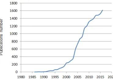
While presenting some of the current applications of AFM technology, it is important to note these are just a few of the many applications and the present research on a topic that gained a lot of relevance over the last 20 years as can be shown in Figure1.1, which gives the general tendency.

Figure 1.1: Number of papers published each year, the data was acquired from a Pubmed search using AFM.

Besides the construction of a quartz sensor AFM, the thesis will also be focused on the study of mechanical properties at the micro and nano level. Using nanoindentation techniques like the PeakForce QNM [9], but also novel techniques such as harmonic force microscopy [10], the AFM instrument it capable of successfully increasing our knowledge on complicated diseases, such as the Parkinson’s disease [11] or Alzheimer’s [12].

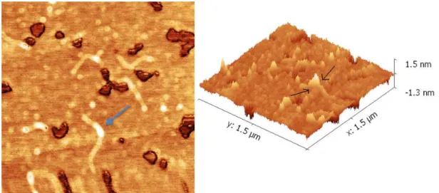
To use an AFM but specially to build one, it is necessary to be aware of the several subtleties of practical use, for that reason I took a 4-5 weeks "internship"in July of 2016 at the physics department of "Faculdade de Ciências da Universidade de Lisboa", to learn more in detail and to get comfortable with those subtleties of practical use. During this time I made topographic images of DNA plus protein (Haa) samples, an example can be seen in Figure 1.2. Presumably the curvilinear shape, being pointed by the arrow, corresponds to the DNA segment. In turn, the globular shape viewed in the figures seems to correspond to the protein attached to the DNA segment forming a complex.

In this experiment, the samples provided had a section of DNA previously ampli-fied which means, to select the region of interest and expressed (production of several

1 . 2 . B R I E F T H E O R E T I CA L R E V I E W

Figure 1.2: Topography of protein DNA complexes in 2D and 3D images, both with 1.5

µm on each side.

copies) with the intention of corroborating the formation of complexes (the binding inter-action between DNA and the protein) visually. More specifically this protein, which was overproduced should form a complex at about one third of the DNA length.

This work was important to get some experience, although constructing an AFM with a different setup from scratch, while using a different type of sensor, was altogether a new

challenge.

1.2 Brief theoretical review

To build an AFM, an understanding of the instrumentation and processes involved is needed, as well as knowledge on the forces involved in the tip-sample interactions. Fur-thermore, knowing what variables will be measured and how they will behave regarding different interactions, can be of great importance. This section was written to make a

brief observation of the theoretical concepts in play.

An effective way to start discussing the theory concept behind the technology of an

C H A P T E R 1 . I N T R O D U C T I O N

When the resulting force is whithin its attractive range, as well as the tip-sample distance is under a certain value, an incident called jump-to-contact can occur [13] (where the tip becomes attached to the sample), there are of course many other factors related to this incident, for example, tip stiffness and other forces, like the capillary forces.

Figure 1.3: Plot of Lennard-Jones potential function, adapted from [14].

The forces involved in tip-sample interactions are:

• Van der Waals Forces- There are several forces that are considered Van der Waals

Forces, such as the ones that come from the London dispersion which is the weakest. These are related to electrostatic interactions between two permanent charges in atoms or molecules.

• Chemical Forces - These occur when the tip is sharing electrons or exchanging

electrons with the surface, if a chemical bond is formed it usually dominates the interaction.

• Contact Forces- Associated with the short range repulsive forces explained by the Pauli exclusion principle, but also with the electrostatic interaction between two charged particles.

• Magnetic Forces - These forces are considered a long-range interaction and they

can be both attractive or repulsive forces.

• Capillary Forces - When there is a confined configuration at the nano scale the

effect resultant from capillary condensation will be present [15]. This strong

attrac-tive force can cause discontinuities in the force-distance curves.

• Viscosity Forces- These forces are influenced by the cantilever’s speed and

geome-try, as well as the sample surface viscosity [16]. Due to their low intensity at long range they are not so relevant in the attractive region but more at close range, in the repulsive region.

1 . 2 . B R I E F T H E O R E T I CA L R E V I E W

The variables that are being measured in a traditional AFM tapping mode, are the amplitude and phase of an oscillating cantilever. While the tip moves, the resulting force from the tip-sample interaction determines the amplitude and phase of the tip, that is oscillating near its resonant frequency. These variables are related to the excitation frequency as it can be seen in the following expressions 1.1 and1.2, where γ is the

damping constant,ωexc the excitation frequency, k is the spring constant, m the mass of

the cantilever andA_excthe amplitude of the oscillation of the cantilever when excited at

ωexc. The deduction and reasoning behind these equations are of paramount importance

for the experimental work in this dissertation and they will be studied further ahead in section4.1.

A= kAexc

q

(ωexcγ)2+

k−ω2excm

2 (1.1)

ϕ= arctan ωexcγ ω2excm−k

!

(1.2)

The interaction changes the natural frequency of the system that goes from ω0 =

√

k/m to ω0 =

p

(k+ki)/m. If the interaction is attractive ki will be negative and the

resultingksmaller, which will create a resonance frequency shift, as the shift occurs but

the excitation frequency remains the same, the amplitude for that specific frequency will be significantly different, as it can be observed in Figure1.4.

Figure 1.4: Natural frequency shift and its implications in amplitude, adapted from [17].

The amplitude is not the only variable that will change as the resonance frequency changes, the phase will also suffer a significant variation much like the amplitude as it

C H A P T E R 1 . I N T R O D U C T I O N

Figure 1.5: Frequency shift in attractive interactions and its implications in phase, adapted from [18].

1.3 Advantages and disadvantages of a quartz crystal sensor

AFM

What follows is a summary on the advantages of using a quartz crystal sensor AFM in comparison to a commercial AFM, based in literature. Since this AFM doesn’t require an optical system, it inherently avoids problems where the radiance from the diode can be affected by outside light. In the early 2000s, the diode laser was also being a factor in

increasing thermal drift and noise from thermal mode hopping which was the limiting source of noise [19]. Although presently it is not as problematic as before, it still adds thermal noise to the system.

Besides requiring less instrumentation, the quartz crystal sensors are also cheap in comparison with the commercial cantilevers. Another great advantage is the non-contact approach, which helps preventing tip and sample damage, something that is particularly useful when dealing with fragile biological samples [20].

To achieve extremely high resolution, high vacuum and low temperature (4.2K) is necessary, which often comes with complex cooling and pumping systems to achieve said vacuum and low temperature. In this type of set up the simplicity of the quartz crystal sensor AFM presents, is a big advantage. Which is why quartz crystal sensor AFM is seeing increase use in high resolution low temperature (LT), ultra-high vacuum (UHV) AFM [21]. Figure1.6adapted from article [22], presents the image of a molecule, acquired with one of these high resolution AFMs while using a tuning fork as a sensor in aQplus

configuration.

Yet another advantage of the tuning fork is that, since it is very stiff, it also avoids

jump-to-contact, which is an incident that has many unfavourable implications in AFM studies. The cantilevers from traditional AFMs have to be soft enough to deflect, but this means that when doing nano indentations it is hard to know how much of the signal is indentation and how much is deflection, which is a problem the tuning fork does not have.

On the side of the disadvantages, there has not been reported a quartz crystal sensor

1 . 3 . A DVA N TAG E S A N D D I SA DVA N TAG E S O F A Q UA R T Z C RYS TA L S E N S O R A F M

Figure 1.6: High-resolution AFM topographic image of Diisononyl phthalate adapted from article [22].

capable of performing very high-speed imaging, where the time per frame on a 250 nm scan range is close to 45 milliseconds [23]. This order of magnitude in time is necessary to study bio-molecular processes that can occur in milliseconds, which means a quartz crystal sensor AFM cannot observe some of the reactions in real time, but only the final result or the average state just like a common commercial AFM.

C

h

a

p

t

e

r

2

S ta t e o f t h e A rt

2.1 Instrumentation

Unlike the laser based AFM, the quartz sensor AFM doesn’t require an optical system. Instead of a laser and a photo sensor, it uses a quartz crystal that can be used as a sensor and an actuator. The initial AFMs with such a setup used a quartz tuning fork, and presented a noise level equal to the laser-based AFMs produced at the same time [19].

While the optical-deflection based AFM uses aProportional-Integral-Derivative (PID)

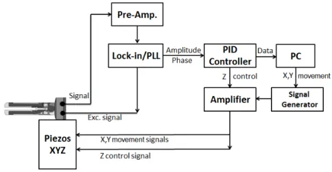
controller, with the function of stabilizing the distance between the tip and sample, the quartz sensor AFM can use aPhase-Locked Loop (PLL)controller in addition to the PID. This system allows to stabilize the phase of the input signal by maintaining the phase of the output signal correlated to the "initial phase"in a loop. A simplified scheme of the components used in the AFM previously described can be observed in Figure2.1.

C H A P T E R 2 . S TAT E O F T H E A R T

The quartz crystal can act as an actuator by exciting it with a drive signal, which can be called input signal, and thus moving the tip attached to one of the crystal’s prongs. In the loop system this drive signal is influenced by the response of the tip, which is the output signal of the crystal/sensor. By monitoring the phase of the drive signal and the output signal’s phase in a loop with a Phase-Sensitive Detector (PSD)and maintaining their correlation the PLL is achieved [19].

The use of PLL in AFM emerged in 1997, and a few years later AFMs using quartz sensors expanded to studies in vacuum where atomic resolution is easier to achieve. This article reports the first atomic resolution attained with an AFM quartz sensor [24], it also introduces a few important improvements that quickly became popular, one of the most important would be the "QPlus"configuration, where one of the prongs of the fork is held fixed, as it can be observed in Figure 2.2. That wasn’t the only configuration that improved the results though, theLength Extensional Resonator (LER), was another quartz sensor AFM that achieved atomic resolution, also known as the "needle sensor".

Figure 2.2: Photograph of the Qplus configuration [24].

One component that both the quartz sensor AFM and the traditional AFM requires, is the transimpedance pre-amplifier or in some cases a charge amplifier. In the most common AFMs it might even require several pre-amplifiers for each quadrant of the photo sensor.

In the case of the quartz sensor AFM it needs a pre-amplifier because the quartz crystal acts like a sponge, when it "contracts"it sends electrons, and when it "expands"it "pulls"electrons, what this means is that while acting as a sensor the quartz crystal will send a very small electric signal that needs to be converted with a gain to voltage. The transimpedance pre-amplifier is responsible for making this conversion and amplification, although simple, this component requires attentive planning. The transimpedance pre-amplifier is responsible for the magnitude of the output signal (after amplification) but also for the addition of noise during said amplification. Article [25] compares the use of a charge amplifier to a transimpedance pre-amplifier and shows that for higher operating

2 . 2 . T E C H N I Q U E S F O R T H E S T U DY O F N A N O - M E C H A N I CA L P R O P E R T I E S

frequencies, like the ones used with LER the charge amplifier presents less noise than the transimpedance pre-amplifier. These are the type of considerations that will be taken into account when choosing the components.

Fast-forwarding to the beginning of 2013 it was reported an AFM quartz crystal sen-sor [2], with an imaging speed 5 times faster than that of a traditional AFM machine, one of the big differences between this one and the previously mentioned, is that instead of

using a fork shaped sensor, cylindrical quartz crystal was used with a resonant frequency of approximately 3.58 MHz, where a tungsten tip will be glued, it is notable that this tip is much larger (millimeter size) than the ones commonly used (micrometer size), this allows an easier integration with a manipulation system, so that manipulation and imaging can be done simultaneously, as well as different sample access approaches.

2.2 Techniques for the study of nano-mechanical properties

As discussed in chapter1.1, knowing the nano-mechanical properties of the materials, is important in several subjects from biology to the study of cement materials.

There are several techniques for the study of nano-mechanical properties, but most can be associated with one of three techniques. The first AFM technique to produce results in the search of mechanical properties was the Force-Volume [26,27] now evolved and known as nanoindentation, this improved version is still being used recently for AFM-based diagnostics research at the cellular level [28]. The other branches are the Multifrequency and the Peakforce. Despite the appearance of the Multifrequency and the Peakforce being in response to some limitations of the Force-Volume there’s certain aspects there are common to all. All these techniques revolve around getting force-curves, also known as force-distance curves, to which a mathematical model will be applied.

At the present time, the most used model to find the Young’s modulus (from where the mechanical properties will be deduced) in a material, is the Hertzian contact model [29], which will be analysed and discussed in chapter4.

Even though nano-indentation is widely used, there were other techniques that ap-peared in response to the Force-Volume limitations and that are regularly used, such as the Multifrequency or the HarmonicForce technique. To briefly describe this technique, it starts with the rough approximation, that the cantilever and tip can be considered a simple oscillator where position can be described by the expression2.1, wherez0is the

always present static component,Athe amplitude of oscillation andφthe phase shift.

z=z0+Acos(ωt−φ) (2.1) Making a more precise description of the system, the harmonics induced by non-linearity eff_{ects must be taken into account, in addition, since the a tip is attached to}

C H A P T E R 2 . S TAT E O F T H E A R T

frequency of the high-frequency components (Harmonics) andAnthe amplitude of each

contribution.

z=z0+ N

X

n=1

Ancos(nωt−φn) (2.2)

By considering the information given by several modes, the multifrequency technique can work at much higher operation frequencies than Force-Volume, while still considering the non-linearity effects.

In this dissertation, the technique used is nanoindentation, so its procedure will now be described. The first step to perform nanoindentation is to determine and find the region that one intends to study, to this effect, a normal microscope or AFM imaging can

be used. The tip should be placed above said region and a trigger-value must be defined, this can either be the target value of the indentation depth or a limiting amplitude value to signal the end of the measurement. The tip will approach the sample until the trigger points are achieved, by which point the tip stops, the distance is registered and the tip will retract. During the tip movement, the "force"is constantly being recorded, which will provide the distance-force curve. A good example to show and discuss a generic distance-force curve is shown in Figure 2.3. In this figure is possible to observe the previously mentioned jump-to-contact effect from the point 1 to point 2, then as the Z

height decreases, there is an increase in tip deflection, the tip is then under the eff_{ect of}

adhesion, which is why there’s a jump from point 4 to point 5 where the force is sufficient

to release the tip.

Figure 2.3: Example of a force-distance curve [31].

The main problem with the first method of nanoindentation, Force-Volume, was time and spatial resolution. The operation frequency was between 0.5 Hz to 10 Hz per pixel [32], and the control signal for the Z position of the tip was triangular which meant that if a higher operation frequency was used there would start occurring irregularities caused by resonance effects originated by the inflection points of the triangular signal.

2 . 2 . T E C H N I Q U E S F O R T H E S T U DY O F N A N O - M E C H A N I CA L P R O P E R T I E S

Because of these limitations new techniques like the PeakForce were developed. The Fig-ure2.4shows the evolution in ramp frequency or operation frequency from Force-Volume to PeakForce.

Figure 2.4: Comparison between the acquisition times of Force Volume and Peak-Force [31].

By having a much higher ramp frequency the Peakforce technique gains advantageous similarities to the topography technique tapping mode, which is not affected by lateral

forces, providing a higher resolution. However, in contrast with tapping mode, the Peak-Force doesn’t use frequencies close to the resonance frequency and by doing so, it avoids the necessity to use filters that often are needed in dynamic resonant systems. In practical terms, this means there must be special attention in knowing the resonance frequency of the system to guarantee that there will not be interference with the operation frequency. The main difference between PeakForce and Force-Volume is the operation signal, which

allows the PeakForce ramp frequency to be higher. Instead of a triangular signal that can cause resonance eff_{ects, the PeakForce uses a sinusoidal signal with smoother inflection}

C

h

a

p

t

e

r

3

P r o j e c t a n d D e s i g n o f t h e A F M

The method employed in the development of this dissertation, was based in breaking down the main objective into many smaller and more manageable ones, and then defining the necessities and constraints applied to each one of them. The focus of this dissertation was the construction of a low-cost AFM based on a quartz crystal sensor, capable of operating at the same or higher level than a commercial AFM, this should be done by integrating components already available, while developing the others.

As a set goal, the AFM should have the capacity to move 30 micrometer on the X and Y axis, since this allows the observation of cells, which are usually the biggest subjects of interest to study with an AFM. Furthermore, it should have a range of 10 micrometer on the Z axis, to cover the respective height of the subjects of interest. One of the other features that the AFM is expected to have, besides being able to use a quartz crystal sensor, is to incorporate the traditional beam deflection sensor through the use of a cantilever and laser, however, in this work the implementation of such a system will not be discussed. Finally, all design decisions and incorporation of electrical components should try to pursue an economical use of the resources available.

To design and have a visual support for the planning of the AFM,Computer Aided Design (CAD)was used, more specifically the softwareSolidWorks.

3.1 Choosing the tuning fork

Choosing the right quartz crystal sensor is of critical importance in the quality of the acquired signal and the first decision to be made, was choosing between using a length extensional resonator (LER), or a tuning fork, which can be observed in Figure3.1.

C H A P T E R 3 . P R O J E C T A N D D E S I G N O F T H E A F M

Figure 3.1: a) Length extensional resonator [25]. b) Tuning fork with a ruler on the background.

much like the tuning fork, when one prong of the LER moves the other prong moves as well, maintaining the center of mass position constant. In this work, the tuning fork is the most appropriate sensor, because it is more accessible as it is mass produced for watches and can be acquired for a low price. This has extra value in the AFM industry, because the sensors are usually very fragile and expensive. It is still notable that despite being very cheap, the tuning forks are still very sensitive and can achieve atomic resolution just like the LER, as mentioned in section2.1.

There are several tuning forks with different shapes and sizes, which meant a detailed

analyzes was needed to determine, which of the available tuning forks on the market would be the most appropriate for AFM. Defining the equation that would allow to calculate the expected sensitivity of each tuning fork is not trivial, so given the time constrains inherent to a dissertation a qualitative approach was preferred instead of a quantitative one.

In the article [24], Giessibl presents the expression3.1for the sensitivitySof a tuning

fork in the QPlus configuration. Whered21 is the piezoelectric coupling constant for

quartz,L_ethe length of the electrode,Lthe length of the prong andtthe thickness of the prong. If a rectangular parallelepiped shape is assumed for the prong, thenK the spring

constant of the prong is given by the expression3.2as found in article [33].

S= 12d21KLe

(L−Le2))

t2 (3.1)

K= Ewt

3

4L3 (3.2)

Since the expression3.1 was deduced for one prong of the tuning fork, because in

Qplusthe other prong is immobilized, it will not make for an accurate quantitative

eval-uation of a tuning fork with two prongs. However, the sensitivity or in other words, the charge generated by a strain in one prong, is the same. The only difference, is that in

the normal configuration of the tuning fork, both prongs are moving, and by doing so,

3 . 1 . C H O O S I N G T H E T U N I N G F O R K

have an additional signal source. What this means, is that although we can’t calculate the true sensitivity of a tuning fork with this method, it is still possible to compare the sensitivities generated by the interaction with the sample using the equation 3.1. The signal-to-noise ratio is another factor important to consider, and the main noise sources at ambient temperature, are the thermal detector noise and the oscillator noise [25].

To calculate the sensitivity with the expression previously presented the tuning forks dimensions andK are needed, and since theK for two coupled prongs is very different

from theKof one prong the expression3.2shouldn’t be used. Many approaches were

con-sidered to calculate the tuning fork’s spring constant, and after reviewing the literature many discrepancies were found. Discrepancies such as, while some articles report that the cantilever model minimizes the true spring constant [34], others find it, overestimates it [35] and there were others incoherencies that were also noted and reported in article [36]. However, something that the last three cited articles have in common, alongside most of, if not all the scientific community, that publishes on this subject, is the consensus around theCleveland Methodwhich allows to calculate the effective spring constant after

adding a small mass on the tip of a micro cantilever [37]. Despite its accuracy this method required for a new experiment to be made with each of the tuning forks, and since there were time constraints as well as this being a qualitative approach another method was selected.

The method selected is called the Geometrical Methodand it was presented in [36],

where it was compared to theCleveland Method, and found to have an 8.7 percent discrep-ancy, for a tuning fork with a resonance frequency of 32kHz. Given how different the

values were expected to be, this level of error would not impact the qualitative compari-son of the tuning fork’s propensity for being used as an AFM sensor, and as such, it was the one employed. The expression presented in the article for the method was3.3, where

f0is the resonant frequency of the sensor,Eis the Young’s modulus of the quartz andρ

its density, whilewis the width andt the thickness of the tuning fork’s prongs.

K= 7.66wEρ3

1 4₍

tf0)

3

2 (3.3)

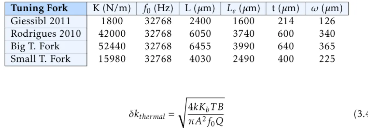
With this equation, theK of the big and small tuning forks were calculated, these val-ues are presented in table3.1. Also presented in the table is theK value of theQplus

sen-sor of Giessibl for reference. The Rodrigues 2010 was already available at the laboratory, while the large tuning fork (DS 26 from microcrystal switzerland) and the small turn-ing fork (DS 10 from microcrystal switzerland) were purchased and have their datasheet available online.

Now all the values necessary to calculate the sensitivity are available. However as reported in article [25], the figure of merit for a sensor is not just the sensitivity, but thek

C H A P T E R 3 . P R O J E C T A N D D E S I G N O F T H E A F M

Table 3.1: Table with the dimensions and constant springs of four diff_{erent tuning forks.}

Tuning Fork K (N/m) f0(Hz) L (µm) Le (µm) t (µm) ω(µm)

Giessibl 2011 1800 32768 2400 1600 214 126 Rodrigues 2010 42000 32768 6050 3740 600 340 Big T. Fork 52440 32768 6455 3990 640 365 Small T. Fork 15980 32768 4030 2490 400 225

δkthermal=

s

4kK_bT B

πA2f0Q (3.4)

Where K_bT is the thermal energy, A the amplitude, and B the bandwidth which is dependent on the component that will amplify the tuning fork signal, and for the purposes of being able to compare the results of this theoretical study with the results of Giessibl in [25] the same value of 1 Hz was assumed, throughout all calculations of this section.

Even though less impactful at ambient temperature than the thermal noise the oscil-lator noise must also be considered and its expression is present in3.5, wherenamp, refers

to the noise density of the pre-amplifier.

δk_ocs=√2Knamp

QS

√

B

A (3.5)

As expected the sensitivity, or charge generated by a certain deflection gets bigger as the electrodes on the tuning forks get bigger as well. However, having a larger size also means the sensors will be stiffer which increases all noise sources, but something else

needs to be considered, the larger the mass of the tuning forks, the smaller the impact of adding an extra mass to the tip will be. When they are inside their capsules the tuning forks have approximately a Q factor of 50000, but once outside it lowers to approximately 4000, and then, the added tip will lower the Q factor of the sensors again. It was measured a decrease to approximately 1100 in the case of the larger tuning fork, while the smaller tuning fork displayed a decrease to 900. It is important to note the change in the Q factor will depend on tip mass, glue mass and other factors, so without a thorough control of said factors, these values can only be used in a qualitative comparison of the tuning forks. In the table 3.2the tuning fork with the Qplus configuration was placed for reference, when comparing it to the other it is important to note that although the Qplus tuning fork, has one prong glued, thus lowering its Q factor, the quality factor is then artificially increased through a control loop. This means that when all the tuning forks present have a tip glued to them, the Qplus tuning fork will have a Q factor approximately three times bigger than the others, which will contribute to lower noise values.

The values for the thermal noise and oscillator noise calculated in table3.2, are given per√Hz, thenamp is not dependant on the tuning forks but on the amplifier, so for the

purposes of these calculations the amplifierFEMTO was assumed for all, meaning the

3 . 2 . D E S I G N - S CA N N E R

Table 3.2: Table comparing some characteristics of four diff_{erent tuning forks.}

Tuning Fork Sensitivity (µC/N) Thermal N. (mN/m) Oscillator N. (mN/m)

Giessibl 2011 2.80 3.1 0.27

Rodrigues 2010 50.60 25.6 1.05

Big T. Fork 63.12 27.7 0.96

Small T. Fork 19.19 16.9 1.17

n_ampwas 90 _√zC

Hz [38]. In the calculations, an amplitude of 100pm was also assumed in

other to stay coherent with the calculations of [25] so that a comparison could be made.

3.2 Design - Scanner

When building an AFM, the scanner is one of the most challenging parts, not only will it play a big role on the AFM operations and data quality, it was also one of the most complex individual pieces built.

An AFM requires the ability of moving the tip with high accuracy in relation to the sample and the scanner is the piece that will allow the AFM to move or excite the sample, with sub-nanometric precision, and for this AFM it should do so within a range of at least 30µm. When building such a system there are some basic decisions that have to be made. Should the sample move on the X, Y and Z axis while the tip remains in place, or should the tip move while the sample stays still? Besides that, there is a lot to consider between geometrically amplifying the movement, considering costs and other factors that will soon be discussed. As such, this was an iterative process and distinct designs were considered before landing on the final one. Since each have their merit, is it worthy to discuss all of them.

3.2.1 Amplified cylindrical scanner

The design for an amplified cylindrical scanner was the first to be considered, and emerged with the purposed of achieving the quality of a normal scanner at very low cost. In this design the movement on the X, Y and Z axis would be done from the sample, that would be placed on the scanner. To make the movement three piezoelectric actuators would be used in the set up roughly described in Figure3.2.

To make a movement on the Z axis, all piezoelectric actuators simply had to expand and displace the cylinder upwards. At first sight, it might seem unnatural to think of deforming the scanner to achieve displacement, but actually the full displacement equates to 0.01% of the scanner length in this case.

C H A P T E R 3 . P R O J E C T A N D D E S I G N O F T H E A F M

Figure 3.2: Rough design of the amplified cylindrical scanner.

actuators would have to compensate the undesired movement, which was a a disadvan-tage.

On the other hand this system presented a geometric amplification equal toh

r, because

when the actuators expanded, xµm the top of the cylinder would move h_r times more. A

considerable advantage since it allows not only to buy smaller actuators which are less expensive, but also to control the natural gain by assembling a different cylinder with

a different _{h r} proportion. However, the system’s low cost does not make up for its

disadvantages, since a commercial scanner is so expensive that the purchase of small or large actuators, are both economical options in comparison.

3.2.2 Not amplified alfa scanner

Buying a micro-positioning system that could be controlled from the computer, was something to consider, since it is able to make large yet precise adjustments to the scanner position, unfortunately it was an expensive system and in the end we opted to go for a micro metric table already available in the laboratory. This table brought the first design constraints to the scanner, and allowed for a more definitive architecture to be planned, regarding the size and shape. This architecture would have to be assembled onto the micro metric table, and preferably have similar dimension, and since there was no geometrical amplification the actuators would need a length around 30mm to be able to cause displacements of 30µm as previously planned. In Figure3.4, a solution for the

requirements mentioned above is presented, and its design will now be discussed. Before though, it is worth mentioning that the piezoelectric actuators we settled on to make the displacement in the X and Y axis, were thePK2JUP2 piezoelectric stackfromThorlabs.

In opposite to the cylindrical scanner this scanner is not geometrically amplified, meaning that the displacement in the actuators will be equal to the displacement of the sample. The basic description of its operation would be, two actuators expand and contract, with high resolution steps, under a force load and by doing so displace a cube

3 . 2 . D E S I G N - S CA N N E R

Figure 3.3: Top view of the not amplified scanner.

connected to the sample holder. Firstly, the structure has to be secured to the micro metric table and to that end, two screw holes concentric to the table’s holes were made, they can be found above the word scanner in Figure3.4. As mentioned before stability is key, and after screwing the scanner to the table with this two holes the scanner has no movement liberty.

To function properly, the actuators have to be under a certain load, and that load is secured on this scanner through a screw that goes against each actuator, compressing the actuators against the sample-holder-adapter on the scanner (represented in green). Naturally it is intended that when the actuators move, only the sample-holder-adapter moves, otherwise some of the 30µm required displacement would spread out in other

regions of the scanner, that are not connected to the sample, meaning the sample wouldn’t be able move the intended distance. The implications that arise from here, are that one end of the actuators needs to rest on a very stiffwall, in comparison to the other end,

that should rests on a cube with two flexible bars connected to it, called flexures. Since according to the third Newton law the actuator will push the screw back, which in its stead is screwed to the nut, the region behind the nut hole has to be stiff, or in this case,

thick enough to assure the displacement will be done by the cube.

As it is visible in Figure3.4, the scanner has features that allow it to safely and easily incorporate the piezoelectric actuators and its supply cables, which are presented in Figure3.5.

It is important to note that the screws need to be very well centered with the piezo-electric actuators, and have its points flattened to guarantee that there won’t be bending forces that might jeopardize the actuators. Naturally the applied load has to have the same direction as the actuator’s axis of displacement, meaning that the screw holes were centered with the actuators base.

C H A P T E R 3 . P R O J E C T A N D D E S I G N O F T H E A F M

Figure 3.4: Oblique view of the not amplified scanner.

Figure 3.5: Thirty-centimeter-long piezoelectric stack used in the scanner for movement in the X and Y axis.

of these and other flexures, involve a lot of work and theory, furthermore, the process in which they were calculated is important to apply ideal load to the actuators, as it will be discussed in subsection3.2.5. As such, the work related to the flexures, was compiled into one place and can be found in subsection3.2.4.

The scanner was also designed so that the sample holders could be fastened to the scanner, and it accounts for the actuators movement, so that they wont slide out of posi-tion during operaposi-tion.

Relative to the cylindrical scanner, this scanner has the advantage of not requiring additional electronic. However it still presented a disadvantage, the two axis movement were coupled, meaning that as one actuator moved and the cube position altered, the other actuator wouldn’t be under the initially set conditions and the same could be said for the flexors. Although their maximum movement is 30µm, meaning the geometrical

im-plications of that movement might not be relevant, but since a scanner main focus should be precision, we made improvements and designed the scanner that will be presented next.

3.2.3 Not amplified beta scanner

This architecture for this scanner is the culmination of all the precautions and issues discussed previously, although its design might be hard to understand at first, an above

3 . 2 . D E S I G N - S CA N N E R

side view can be seen in Figure3.6.

Figure 3.6: Above side view of this scanner iteration.

This scanner has several features, such as, eight tubes to screw the scanner on the micro metric table, an extruded center to place the sample holder, with four nut holes and screw tubes to fasten it, to mention some. The more important features would be the eight flexures, four for each axial movement and finally two weakened side structures, represented in green. Some of these features are best seen in the under side view of the scanner, shown in Figure3.7, where the piezoelectric actuators are set in place.

Figure 3.7: Bellow side view of the last scanner iteration.

As it is possible to observe, the actuators are set on diff_{erent levels and they will}

ultimately move different parts of the scanner. As mentioned before, the problem with

C H A P T E R 3 . P R O J E C T A N D D E S I G N O F T H E A F M

in its stead the inner shell moves in one direction, as represented by the brown arrows. When the actuator expands, one tip will be against the outer shell that is thick and stiff,

while the other tip will push against a wall of the inner shell, this wall is also very stiffand

its bending is negligible, on the other hand the four flexures are soft by comparison and will bend under the force represented by the other four brown arrows. Since the green structures coming out of the side of the second shell are not connected to the outer shell, both the inner shell and central block will move without any alteration on the central block flexures. Speaking of which, when the actuator with the black arrows expands, one tip will pushes against the inner shell and the other against a wall of the central block meaning once again, that the stiff_{walls will have negligible bending and that the flexures}

to where the black arrows are pointing will be the ones to bend.

Figure 3.8: a)Top view of the scanner with arrows showing how the center moves in relation to each actuator. b)Bottom view of the scanner with same indicators.

This scanner’s architecture allows it to make use of the micro metric table the labo-ratory already had, which was capable of a movement of 30µm in each direction, with minimal steps similar to a commercial one, but for one tenth of the cost it would take to buy one.

3.2.4 Euler-Bernoulli and flexures calculations

The theory and process behind calculating the optimal geometry for flexures was of paramount importance in this work, and the same general idea was applied to every piece that would need a piezoelectric actuator. Since for an actuator to perform the expected displacement this one is required to be under the ideal load. In this work, it meant that every actuator was between a screw with a stiff surface behind and a soft

structure (flexures) somewhere, but to know what force a certain bending of the material,

3 . 2 . D E S I G N - S CA N N E R

will exercise on the actuator, one needs to know the Euler-Bernoulli beam theory whose general equation is3.6. Hereqis a distributed force load across a beam,ω(x) gives the

deflection acrossx,Eis the Young Modulus andI is the moment of inertia of a plane area,

which in this case would be the cross section of the beam.

q= d

2

dx2 EI d2ω

dx2

!

(3.6)

However, if the product ofEandIequals a constant, which would simply mean that

across the beam, these properties remain constant and we are dealing with a uniform static beam, then the following expression3.7can be written.

q(x) =EId

4_ω

dx4 (3.7)

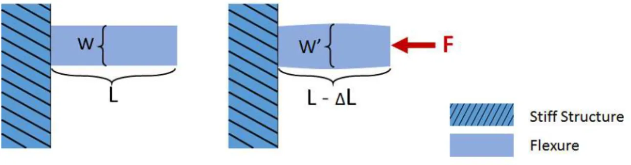
To use this expression, we should first have in mind what geometry the beam will have and where the force will be applied. In this dissertation, there were discussed three main flexures designs. The first being presented in Figure3.9.

Figure 3.9: Scheme of the column flexure, before and after being under a certain force.

The behaviour of this flexure is easier to predict since given its geometry and the direction of the force applied, the relation between force and displacement is given by the definition of the Young modulus, expressed mathematically in equation3.8. Where

δLis the displacement, F the applied force,wandLrepresented in the Figure3.9, are the

width and length,Ethe Young modulus andt the thickness of the bar, not visible in the

2D perspective. This type of flexure was considered for many pieces, such as the scanner and the piece where the tuning fork holder would assemble to, but ultimately it was only used in the Z control stage to test the scanner while other pieces were still being designed or awaiting delivery. The main advantage of this flexure is that the assumptions made on the calculations to predict displacement-force relation, are identical to the geometry and conditions of the flexure in practical use, while the others are approximations.

δL= FL

wtE (3.8)

C H A P T E R 3 . P R O J E C T A N D D E S I G N O F T H E A F M

is a differential equation that requires four assumptions to constrain it and allow for a

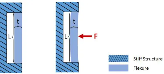
solution to be reached. In its stead, the assumptions depend on the flexure geometry and localization of force applied, so the design of the fixed beam will be presented first, in Figure3.10.

Figure 3.10: Scheme of the fixed beam flexure, before and after being under a certain force.

To solve the differential equations, we need to express the assumptions in

mathemati-cal form, so analyzing the geometry, the first assumption made was that both ends of the beam were fixed, meaning that whenx= 0, the deflectionωwill be zero as well. But not

only will it have no deflection, it will also not have curvature, which means thatω

deriva-tive inx= 0 will also be zero. Another place where we can expect to have no curvature is in the inflection point, precisely where the force in being applied, which in this case is at half length, resulting in,ω′ _at L

2 being zero. The last assumption was the hardest to

grasp and it stems from equation3.7, while assuming that the force load is applied on one point only, at L

2 in the beam. After defining the assumptions the functionDSolvewas

applied in the programWolfram Mathematicato solve the differential equation with the

following boundary conditions:

• ω(0) = 0

• ω′_{(0) = 0}

• ω′₍L

2) = 0

• ω′′′₍L

2)EI=F2

With this method the equation3.9, describing the deflection-force behaviour of the fixed beam was reached.

ω(x) =F(3Lx2−4x3)

48EI (3.9)

3 . 2 . D E S I G N - S CA N N E R

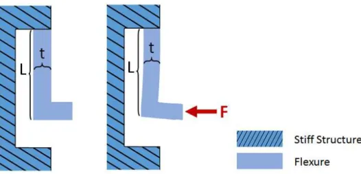
However some pieces, like the final scanner and the piece where the tuning fork holder would be assembled, didn’t mesh well with this geometry, so a last flexure was designed, which can be observed in Figure3.11.

Figure 3.11: Scheme of the cantilever flexure, before and after being under a certain force.

Once again the differential equation needed four conditions to be solved, and since the

cantilever flexure also has one of its sides fixed, the first two boundary conditions of the previous design remain valid. As to the third, since the "head"of the cantilever has a much largert, it can be assumed that its curvature will be negligible, even though the deflection

will be the highest of the whole bar-cantilever. So the third condition will express that, at

x=L,ω′ _{will be zero. Finally, the last assumption is similar to the fourth assumption of}

the previous flexure, but instead of applying half of the force on the halfway point of the bar, the full load force will be applied at thex=L, much like last time, this assumption

is an approximation because the force will be distributed in a small area instead of one point. The boundary conditions used inWolfram Mathematicafor this flexure were the

following:

• ω(0) = 0

• ω′_{(0) = 0}

• ω′_{(L) = 0}

• ω′′′_(L)EI=F

The equation attained with this method was3.10.

ω(x) =F(3Lx

2

−2x3)

12EI (3.10)

In these equations, the dimensions of thickness and width were taken into account by the moment of inertia which is given by t3w

C H A P T E R 3 . P R O J E C T A N D D E S I G N O F T H E A F M

has the Young Modulus of the materials in display, we simply fixed some convenient dimensions and varied the others to attain a result of Xµm, given the ideal load in each

respective case. This ideal force had to be divided by the number of flexures in each direction, and the calculations were made, so that the midpoint of deflection occurred for said ideal force, so that when varying the force, it will average the ideal one.

3.2.5 Applying approximately ideal load onto the piezoelectric actuators

The force load applied to the piezoelectric actuators is one of the crucial factors to take into account when trying to guarantee that the actuators will work as planned. The load will aff_{ect their resonance frequency, which needs to be much larger than the operating}

frequency, because if it is not, it would alter the displacement the actuators are capable of. The load will also affect the actuators maximum displacement possible, meaning that

if ideal load is not secured, they might not reach the necessary displacement.

To apply the ideal load one needs to be able to measure or know the load that is being applied. Ideally, this task would be accomplished by using a sensor plaque, for example, placed between the screw head and the ceramic plate of the actuator, which would measure the force as we applied it. However, that was not possible so we used a high-resolution camera connected to the computer. Initially the camera was held by a device next to the scanner, but when tightening the screws connected to the actuators the macro stage would slightly slide. So we screwed a taller M4 screw to the scanner, and assembled a rod where the camera would be held to. This way, even if the macro stage and scanner slightly slide, the camera will move simultaneously and the image will be stable. This set up can be observed in Figure3.12.

Figure 3.12: Set up used to measure load applied onto the piezoelectric actuators.

3 . 3 . A N OV E L WAY O F CO N T R O L L I N G A P P L I E D LOA D S

The camera allows the observation of the scanner movement during the tightening of the screws. To quantize this movement, a calibration sample whose size of the micro-metric features are known, was placed on top of the scanner and used as reference. In subsection 3.2.4, the displacement generated by a certain force was calculated for the tensors of the scanner, so it was known beforehand that a displacement of approximately 250µm would be needed for and ideal load of 144N to be applied. This load of ideal

oper-ational use, was identified by the companyThorlabsthe manufacturer of the actuators. During the process of assembling the set up and adjusting the calibration sample, there exists a risk of contaminating the calibration sample, so we printed a calibration sample. By using Gimpan image manipulation software, an image was created with

squares separated by 200µm in X and Y, which was the best the printer available could

reliably make, but still within the necessary requirements. We measured the distance between two squares on the computer and moved that distance plus a fourth of that distance securing the 250µm displacement without endangering the calibration sample.

A photo of the printed calibration sample, taken by the camera can be seen at Figure3.13. It is worth mentioning that this is the view of the sample before zoom, since with zoom the camera can show a 1.2mm for 1.2mm image, where only 5 to 6 squares can be seen per line, which was what we used.

Figure 3.13: a) Closer photography of the printed calibration sample. b)Wider perspective of the printed calibration sample on the scanner.

3.3 A novel way of controlling applied loads

Several tests were performed in order to understand if the load applied onto the actuators was even, and if it resulted in equal movement by the actuators. An idea came up, to use the tuning fork as an indirect load sensor. As already presented in the theoretical review section1.2, more specifically in expression1.1, the bigger the excitation amplitude

Aexc, the larger the tuning fork amplitude will be. Since we can monitor the tuning fork

C H A P T E R 3 . P R O J E C T A N D D E S I G N O F T H E A F M

scanner to excite the tuning fork. We stuck a tuning fork holder to the scanner with adhesive tape and introduced an excitation signal with frequency equal to the tuning fork resonance frequency, onto one of the actuators. With zero load, the actuator won’t push the scanner walls and the tuning fork amplitude will be close to zero, but as load is progressively applied, the actuator will displace the scanner more and more, until it reaches its maximum displacement. From that point onward, as load force is continuously increased the actuator will be pressured and not able to displace as much, meaning the

Aexcwill be smaller, and consequently we will measure a lower tuning fork amplitude.

Figure 3.14shows the tuning fork amplitude signal while searching for ideal load, with the method described above.

Figure 3.14: Tuning fork amplitude signal during experiment, where force load onto the actuators is being varied.

It is possible to see that between the plateaus in the graphs, where the force wasn’t being varied, there appears to be hectic zones, those occur, due to coupling between the hand, screw driver and the screw, which end up acting as a damper and source noise to the system.

The method presented in this section can be used with other oscillators in any dis-placement setup, that requires a specific load, as long as it is capable of operating with the resonance frequency of the chosen oscillator. In conclusion, it is possible to guarantee with this technique, that the force applied will be the one that causes the most movement displacement, which is very important not only for the scanner range, but also to secure that both axis move similarly.

3.4 Design - Tip Production Setup

In contrast to the cantilevers of the laser based AFM, there isn’t mass production of tuning forks with tips already glued to them. Although at first this may seem a disadvantage,

3 . 4 . D E S I G N - T I P P R O D U C T I O N S E T U P

the fact that the cantilevers are expensive and fragile means that alternatives should be considered. Regarding the tuning forks as an alternative, they are cheap and the process of making and gluing tips to the tuning forks are of relative ease and economical, which is another advantage of having a quartz sensor AFM.

This stage requires the production of a sharp tip, with the ability to easily glue it to a tuning fork. For this AFM, we were aiming to make tips with 0.5 to 1 millimeter of height, presenting a conical shape where the base diameter would be 0.125 mm and the apex of the tip on the cone in itself having, less than 100 nm. In literature, there are already extensive studies on how to make sharp tips that can be used for,Field Ion Microscopy (FIM),Scanning Tunnelling Microscopy (STM), AFM and other areas, through chemical etching [39].

In this work, thelamellae drop off techniquewas employed, whose set up can be

ob-served in Figure3.15. This technique requires NaOH (sodium hydroxide) with a molar concentration ranging from 2M to 3M to act as an electrolyte, two rings of stainless steel, to act as electrodes, that won’t deteriorate while the chemical etching takes place. The tips are obtained by using a tungsten wire, glued to the tuning fork, which in this work had a radius of 0.125 mm and applying a DC voltage that can go from 2V to 9V to the rings. Then current will flow through the wire prompting the chemical etching reaction, that is mostly described by chemical equation3.11, to take place creating two tips.

W+ 2H2O+ 2N aOH→3H2+N a2W O4 (3.11)

The "recipe"described, including molar concentration and DC voltage values, was consulted from article [40]. The wire’s own weight will pull the lower part down, helping the tip formation and impacting its shape, once the region where the etching is taking place gets thin enough, it will break apart creating two tips. This means the etching process will halt on its own, since the tungsten wire won’t be connecting both rings and there will be no current flowing between the NaOH and the tungsten. This is an advantage since in other systems, like the one where only one ring is used, the user is required to cut the power supply, usually by adding an additional software program control, to guarantee that the etching on the upper part will stop, at the same time as the power part.

The first step in the process of producing a tuning fork with a tip, is gluing a very small wire to the tuning fork, which requires a lot of precision to get the right position and with the right angle to the tuning fork. Besides that, every element of the set up needs to be held at the right distance, with stable connections between the rings and the power supply. As such a set station capable of fulfilling the requirements had to be built.

3.4.1 Board production planning and design

C H A P T E R 3 . P R O J E C T A N D D E S I G N O F T H E A F M

Figure 3.15: Representative scheme of the etching technique used.

used. This table with four M2 holes, can have a structure fasten on top of it. This same structure, needed to have a compartment where a 0.125 mm wire could be kept straight, and a place to allocate the rings that would have to be firmly connected to the power supply. The design of the resulting structure is represented in Figure3.16.

Figure 3.16: Board that holds the wire compartment and rings for the chemical etching process; a) top view and b) side view.

To hold the wire straight the needle of a normal syringe was glued to the manufactured board, that is represented in the drawing as the dark blue cylinder3.16. This is where the wire will be placed pointing up, when the tuning fork with a very small drop of glue, stuck to a height controller system comes down to attach the wire to the tuning fork.