Linear Dynamical Systems
Performing the Open-Loop and Feedback Control Policies in Just-in-Time Context
Guilherme Gomes da Silva
Programa de Pós-Graduação em Engenharia
Elétrica
Optimal Control Synthesis for Max-Plus
Linear Dynamical Systems
Performing the Open-Loop and Feedback Control Policies in Just-in-Time Context
Guilherme Gomes da Silva
Thesis submitted to the Programa de Pós-Graduação em Engenharia Elétrica (PPGEE) from Universidade Federal de Minas Gerais (UFMG), as a partial condition for ob-taining the PhD Degree in Electrical Engineering.
Thesis Evaluation Committee:
Prof. Dr. Carlos Andrey Maia - Advisor (DEE (UFMG)) Prof. Dr. João Carlos dos Santos Basílio (COPPE (UFRJ))
Prof. Dr. Valter Júnior de Souza Leite (Mecatrônica (CEFET-MG)) Prof. Dr. Ricardo Hiroshi Caldeira Takahashi (DMAT (UFMG)) Prof. Dr. Leonardo Antônio Borges Tôrres (DELT (UFMG)) Prof. Dr. Vinícius Mariano Gonçalves (DEE (UFMG))
Primeiramente agradeço à Deus pela força, proteção e bençãos em cada dia de minha vida.
Agradeço à minha esposa Juliana, pelo amor, paciência e apoio ao longo de toda essa jornada. Ao meu filho, Luís Miguel, que no término da jornada, com seu jeito de ser e olhar, chegou trazendo mais força e incentivo para conclusão deste trabalho.
Aos meus queridos pais, pelo amor, ensinamentos e proteção enviados, com toda certeza, de algum lugar bem próximo à Deus. Minha família (não citarei nomes devido ao grande número de pessoas, mas todos foram muito importantes), a qual foi fundamental para esta conquista, sendo sem dúvidas a base fundamental de minha vida. Agradeço à Tia Regina pela guarda e proteção, sempre com palavras de incentivo em momentos oportunos. Aos meus avós, exemplos de vida e superação, na casa dos quais, por grande parte de minha vida, sempre tive lar digno e acolhedor. À minha irmã Fernanda, obrigado por tudo.
Agradeço especialmente ao meu orientador, Prof. Dr. Carlos Andrey Maia, pela orientação e ensinamentos que vão além do conteúdo desta tese. Agradeço à confiança desprendida desde o início dos trabalhos ainda no mestrado. Serei sempre grato.
Aos membros do Programa de Pós-Graduação em Engenharia Elétrica da UFMG, técnicos e docentes, em especial ao coordenador do programa Prof. Dr. Rodney Rezende Saldanha, que sempre me ajudaram em várias esferas.
À CAPES e a UFMG pelo apoio financeiro.
Nunes Almeida pelo apoio incondicional ao longo desses anos.
Agradeço aos meus amigos do movimento escoteiro, Tarcisio, Rainer, Mar-lon, Marcos, Artur (em memória) e Ronaldo. Amigos que escolhi para irmãos. Agradeço também ao grande amigo Geraldo Antero.
À aqueles que não citei mas que de algum modo fizeram parte desta conquista. A importânica de todos será sempre lembrada.
Finalmente, sou grato à todas as pessoas que de alguma forma fizeram parte desta importante conquista em minha vida.
Firstly I thank God for the strength, protection and blessing in every day of my life.
I’d like to thank my wife Juliana for her love, patience and support throughout this journey. My son, Luís Miguel, who at the end of the journey with his way of being and gentle eyes, came into the world bringing me the strength and encouragement to fulfill complete this task.
I’d like to thank my dear parents for their love, teaching and protection.They sent me from somewhere very close to God. The whole family (I will not write any names due to the great number of people, but everyone was really impor-tant), which was crucial for this achievement. Thanks to Aunt Regina for her custody, protection, always with encouraging words at appropriate times. To my grandparents, my role model, in whose house, for a long time of my life, I always had a dignified and welcoming home. I’d like to thank my sister Fernanda, for all she has done to me.
Special thanks to my advisor, Prof. Dr. Carlos Andrey Maia, for the guidance and teachings that go far beyond the content of this thesis. I thank you for believing in me from the start of this project, which is being developed since the master degree course. I will always be grateful.
To the members of Programa de Pós-Graduação em Engenharia Elétrica (PPGEE) from Universidade Federal de Minas Gerais (UFMG), technicians and professors, especially the program coordinator Prof. Dr. Rodney Rezende Saldanha, who always helped me in various spheres.
To CAPES and UFMG for financial support.
es-Leonardo Adolpho Rodrigues da Silva and Cassia Regina Santos Nunes Almeida for the unconditional support over the years.
I thank my friends from Boy Scouting, Tarcisio, Rainer, Marlon, Marcos, Artur (in memory) and Ronaldo. Friends whom chose as brothers. I also thank my great friend Geraldo Antero.
I thank all those ones that I haven’t mention by name but somehow were part of this achievement.
Max-Plus Linear Dynamical Systems are systems modeled by Timed Event Graphs (TEG) whose dynamic can be described by Max-Plus Algebra. This the-sis deals with control policies applied to the Max-Plus Linear Dynamical Systems. A new multi-objective formulation to control this class of systems is proposed. This formulation is based on optimization problems and it is possible to consider non-convex constraints (in conventional algebra) in the formulation. Two control policies are obtained from the general problem. The first one is the open-loop Just-in-Time Control, which can be developed either in finite horizon or in infi-nite horizon aiming to saving resources and the optimal control. The necessary and sufficient conditions to solve the problems are presented, as well as the dis-cussion about the computational complexity of the proposed methods in order to solve them. Some concepts on max-plus algebra are used, such as (A,B)-invariant sets, Residuation Theory and the Theory of Semimodules. Due to computational complexity of general method of solution, algebraic properties are used to solve an important class of problems of practical interest. The second control policy is the Feedback control in Just-in-Time context. The conditions for the existence of a feedback matrix are presented. It is also presented a way to find the greatest feedback matrix in order to comply with deadline dates for the system output. At the end of each control problem, numerical examples are developed to illustrate the applicability of the proposed methodologies and the relevance of systems here addressed.
Dy-1 Introduction 1
1.1 Brief Contextualization of the Thesis . . . 1
1.1.1 Thesis Justification . . . 7
1.2 Publications . . . 12
1.3 Organization . . . 13
2 Preliminary Concepts 15 2.1 Discrete Event Dynamic Systems . . . 15
2.2 Graphs . . . 18
2.3 Petri Nets . . . 21
2.3.1 Timed Event Graphs . . . 28
2.4 Dioids and Max-Plus Algebra . . . 30
2.4.1 Lattice Properties of Dioids . . . 31
2.4.2 Max-Plus Algebra . . . 32
2.4.3 Graphs and Matrices . . . 34
2.4.4 Systems of Linear Equations . . . 38
2.4.5 Spectral Theory of Matrices . . . 39
2.5 Residuation Theory . . . 47
2.6 Theory of Semimodules . . . 53
2.6.1 Finding All Solutions to Equation 𝐴𝑥=𝐵𝑥 . . . 54
2.7 Modified Alternating Algorithm . . . 59
2.7.1 Dealing with Equations such as 𝐴𝑥⊕𝑐=𝐵𝑥⊕𝑑 . . . 63
2.8 Conclusion . . . 65
3 Control Problem Formulation and Optimal Synthesis 67 3.1 Introduction . . . 67
3.2 General Optimization Control Problem Formulation . . . 68
3.3 The Open-Loop Just-in-Time Control Problem in a Finite Horizon 72 3.3.1 Introduction . . . 72
3.3.2 Determination of Minimum Viable Reference . . . 76
3.3.3 Performing the Open-loop in Just-in-Time Control in a Fi-nite Horizon . . . 78
3.3.4 Numerical Examples . . . 88
3.3.5 Conclusion. . . 99
3.4 The Open-Loop Just-in-Time Control Problem in Infinite Horizon 100 3.4.1 Introduction . . . 100
3.4.2 Performing the Open-Loop Just-in-Time Control in Infinite Horizon . . . 101
3.4.3 Complexity Issues. . . 111
3.4.4 Algebraic Results to Compute the Just-in-Time Control in Infinite Horizon . . . 112
3.5 Feedback Control Problem . . . 127
3.5.1 Introduction . . . 127
3.5.2 Performing the Feedback Control Problem . . . 129
3.5.3 Numerical Examples . . . 132
3.5.4 Conclusion . . . 141
3.6 Synthesis of Controllers. . . 141
4 Final Discussion 143 4.1 Conclusion . . . 143
4.2 Future Works . . . 145
i.e. That is (“id est”)
e.g. For example (“exempli gratia”)
Z Relative integer numbers
Zmax Max-Plus Algebra (Dioid)
⪰ Greater or equal than (natural order)
⪯ Less or equal than (natural order)
⊕ Max-Plus addition
⊗ Max-Plus multiplication
+ Traditional sum
− Traditional subtraction
AT Transpose ofA
I Max-Plus Identity Matrix
An nthpower ofAin Max-Plus Algebra
∘
∖ Left residuation
∘
/ Right residuation
ImA Image of matrixA
∧ Minimum operator (Ex: 2∧5 = 2)
⋀︀
Matrix greatest lower bound (Ex: [1 5]⋀︀
[3 2] = [1 2])
⊤ Top (largest) element in Max-Plus Algebra
ε Zero element in Max-Plus Algebra
e Identity element in Max-Plus Algebra
|ρ|l Length of pathρ
Introduction
1.1
Brief Contextualization of the Thesis
Technological advances have increasingly required new techniques for the syn-thesis and control of complex systems. Some of these systems have man-made operational rules and the rules are related to events, observable or not observable. Events are such as the beginning of a machine operation, a resource enters a sys-tem and a server starts the customer service. The events are discrete by syssys-tem definition, i.e., the events do not have a time duration. This class of systems is classified as Discrete Event Systems (DES).
some works as Tropical Algebra), because the algebra uses the maximization and addition operations from conventional algebra. So, the systems modeled by a TEG and described by max-plus algebra are called Max-Plus Linear Dynamic Systems (MPLS).
The nonlinear systems based on events cannot use the classical theory of con-trol because the classical theory deals with continuous systems in time. The main importance of max-plus algebra is the fact it describes complex nonlinear systems. That is done in a linear way by using space state equations.
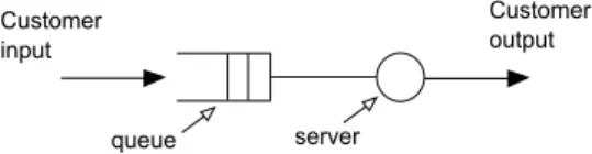
In order to illustrate the statements described in the previous paragraph, consider the queuing system illustrated in Figure 1.1. There are different sys-tems that can be viewed as queuing system, for example, production syssys-tems, communications and computer systems, transportation systems, garage systems, airports, and so forth.
The elements of this system are the queue, the server and the customers. The term customer can refer to people, tasks, trucks, pieces, patients, airplanes, e-mail, cases, orders, and so on. The term server might refer to something able to do a service like a receptionist, a machine, a medical personnel, an attendant, a CPU in a computer, any resource that provides service. The queue is the place where the customers must wait by the service because, normally, the capacity of the server is bound, and, in some systems, there is a limit to the number of customers that may be in the queue.
Customer output Customer
input
server queue
It is possible to consider three events driving the queuing system: • eventa: the customer enters the system.
• events: the service starts.
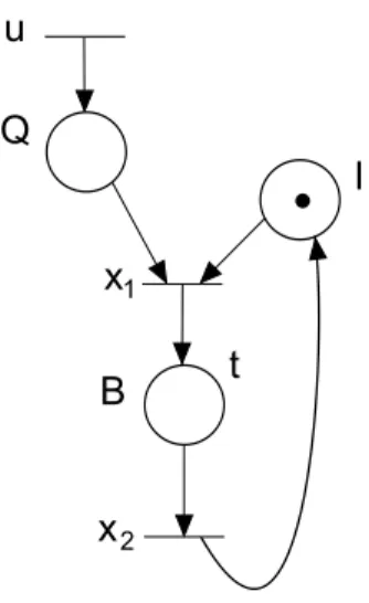
• eventc: the service is completed and the customer leaves the system. The system can be modeled by Timed Event Graphs (TEG), as showed in Figure1.2, representing the events𝑎, 𝑠 and𝑐as transitions (bars associated with
𝑎,𝑠and𝑐). The queue and the server are represented by places (circles)𝑄and𝐵, respectively. The place𝐼 represents when the server is idle or busy, this condition is shown by the token (black circle in place),i.e., when the server is idle there is a token in place𝐼.
a
s
c B
I Q
t
(a)
a
s
c B
I Q
t
(b)
Figure 1.2: Timed Event Graphs. (a)Queuing System A.(b)Queuing System B.
one token in𝐵, indicating that the server is busy.
The event 𝑎is spontaneous and requires no condition to happen, occurring at instant𝑡𝑎. On the other hand, the event𝑠depends on two conditions to happen:
the presence of customers in the queue and the server being idle,i.e., the event 𝑠
can happen at the instant 𝑡𝑠 = 𝑚𝑎𝑥(𝑡𝑎, 𝑡𝑐−), in which the instant 𝑡𝑐− represents
the date when the server is idle by the output of a previous customer of system. Lastly, the transition𝑐requires that the server to be busy and a time𝑡of service, so the event 𝑐 will happen at date 𝑡𝑐 = 𝑡𝑠+𝑡. So a customer leaves the system
at date𝑡𝑐 = max(𝑡𝑎,𝑡𝑐−) +𝑡𝑠+𝑡.
Considering that the system can serve a lot of customers, although just one at a time, the system can be represented, in a general way, by the TEG of Figure
1.3.
x
x B
I Q
t u
1
2
Figure 1.3: Queuing System modeled as Timed Event Graph
transition𝑥2 can also be called output transition𝑦, that represents the date when
a customer leaves the system. In this way, considering the previous statements, the dynamic behavior of the system is described by the following equations:
𝑥1(𝑘) =𝑚𝑎𝑥(𝑢(𝑘), 𝑥2(𝑘−1)),
𝑥2(𝑘) =𝑡+𝑥1(𝑘),
𝑦(𝑘) =𝑥2(𝑘),
being that the integer variable 𝑘 numerates the transitions firing dates, for ex-ample, 𝑥1(𝑘) indicates the instant (date) in which the 𝑘𝑡ℎ customer is accepted
by the server.
The system dynamic behavior in this example could be completely described using the operator maximization (𝑚𝑎𝑥) and operator addition (+). The operator
𝑚𝑎𝑥 is related to the synchronization phenomena and the operator + to the processing time of the process. Then, the behavior of a TEG can be completely described by Max-Plus Algebra, in which the operator𝑚𝑎𝑥is represented by the symbol ⊕ and the operator + is represented by the symbol ⊗. Therefore, the previous equations can be rewritten as:
𝑥1(𝑘) = 𝑥2(𝑘−1)⊕𝑢(𝑘)
𝑥2(𝑘) = 𝑡⊗𝑥1(𝑘)
This queuing systems can be used to compose a complex queuing net and, consequently, it is possible to get equations in max-plus algebra to describe the system behavior.
Based on the previous equations, the max-plus algebra is very relevant and it simplifies the representation of several complex systems because, as previously mentioned, it is able to write non-linear equations (endowed with operator 𝑚𝑎𝑥
and +in conventional algebra) in a linear way.
Besides queuing systems, several systems can be classified as MPLS and use the max-plus algebra to describe the temporal dynamic, as examples, it is possi-ble to mention the manufacturing systems; logistics, transportation and distribu-tion systems; chemical systems; communicadistribu-tion and computadistribu-tional systems; mil-itary and health applications, and so on (Cassandras and Lafortune,2008)(Banks et al., 2005)(Katz, 2007). Therefore, tools and theories used for modeling and controlling these complex systems, in a simple way, are very valuable given the importance of systems.
1.1.1 Thesis Justification
Based on the context previously described, this thesis presents results related to Max-Plus Linear Dynamic Systems. The main results are useful to synthesize optimal controllers in order to make the system respect some constraints. The main objective of the controller proposed in this work is making the system evolve in accordance with the Just-in-Time (JIT) policy, i.e., finding the maximum system input dates in order to comply with deadline dates aiming to develop the minimum cost policy for the inventory. The inventory can be time, money, pieces, and so fourth.
This policy is a management strategy in which the production rate is decided by the demand requires. The main advantage is controlling the inventory costs while still serving customers demand. The control must satisfy some initial con-dition, state variables are subject to some constraints and the control is optimal to the chosen criterion (Houssin et al.,2007).
The objective of JIT control is to find the maximum input dates from a given date 𝑘 = 𝑘′ so that the output dates respect a desirable viable trajectory, i.e., the output dates are less than or equal to the desirable output dates.
Initially in this thesis, a general control problem formulation is proposed. The formulation is developed as a multiobjective optimization problem . Two control policies are derived from this general control problem: The Open-Loop Just-in-Time Control and the Feedback Just-in-Just-in-Time Control policies.
It is important to remark that the control policy choice depends on practical interest and the system features. The distinction between an open-loop control system and a feedback control is important and fundamental. In the open-loop control, the inputs are fixed and independent of output effects (variables of sys-tem), the variables of the system do not have anya posteriori influence in control action. On the other hand, the feedback control uses any available information about the system behavior to adjust the control input.
From the classical control theory, in closed-loop control policy, the feedback makes the system output relatively more insensible to external disturbances and the internal parameter variations of the system, in comparison with open-loop control policy. In this way, it is possible to use some inaccurate components in order to get a precise control of the system. However, considering stability, open-loop control policies are better than closed-loop control policies since the closed-loop control policies can cause oscillations in the output of a stable system (If a system is unstable it will remain unstable for feedback control in classical control theory). Therefore, the feedback can make a stable system becomes unstable.
although the feedback policy is bound in the sense of satisfing some constraints. The open-loop control policies can guarantee optimal performance for any kind of DES system, but it cannot guarantee stability (for more details seeMaia(2003)). To systems in which the inputs are known in advance and there are no distur-bances, the open-loop control systems are more indicated. To systems endowed with unknown parameters and subjected to disturbances the closed-loop control policy is more indicated.
From the general control problem, this thesis presents initially an approach to the open-loop JIT control in finite horizon which is useful to solve some problems. A second approach of open-loop JIT control in infinite horizon is also presented. In order to solve these problems, two issues can be exposed. The first issue is the time computational complexity. As the horizon grows, the time complexity can grow double exponential with the horizon using some methodologies. The second issue is the computational memory. The computational memory to find the solution can be impracticable for some applications depending on the size of the horizon.
In order to deal with the issues previously mentioned, algebraic properties to solve an important class of problems of practical interest are studied. The nec-essary and sufficient conditions to solve these classes of problems are presented. Thanks to these properties, it is possible to find the solution to problems of practical interest.
can be non causal, i.e., there are entries in the feedback matrix less than zero, but a causal feedback matrix can be found from the non causal feedback matrix.
Another control policy of interest is the Feedback Control. Regarding con-strained feedback control problem, several results were obtained for some class of problems. The paper Maia et al. (2011b) aims to find a feedback controller that ensures the system evolution in accordance with semimodule constraints. The methodology to achieve the goal is based on the super-eigenvector of a matrix. The paperAmari and Isabel Demongodin (2012) develops the constrained feed-back controller and the solution is addressed looking for the constrained state equations. The supervisor feedback controllers are calculated and classified ac-cording to their performance, and there is no guarantee for the optimal feedback control. In Maia et al. (2011a) the feedback controller is calculated using an equation that involves the system, the feedback and the constraint matrices. The sufficient conditions to calculate a causal feedback matrix, using the Alternating AlgorithmCuninghame-Green and Butkovic (2003), are presented.
Houssin et al. (2013) deals with feedback control using dioid series (idempo-tent semiring) ℳ𝑎𝑥
𝑖𝑛[[𝛾,𝜎]] in an infinite horizon, however, the control objective
is the opposite of Just-in-Time policy, i.e., the transitions will fire as soon as possible. All works mentioned about feedback control aim to find the smallest causal feedback matrix.
state in conventional algebra. The main importance of semimodules is the fact that all solutions to equations like 𝐷𝑥=𝐸𝑥 belong to a space finitely generated characterized by an image of a matrix (Butkovic and Hegedus, 1984)(Gondran and Minoux, 2010).
The two policies are important in control theory and largely used in many practical applications. In this sense, the formulation deals with the direct real-ization for the problem,i.e., dioid series are not applied because the applicability of direct realization is simpler and easier to manipulate in practice. Unlike some previous papers on the subject, this thesis presents the discussion about the necessary and sufficient conditions to find a solution to the problems.
Lastly, the author hopes that the results published in this thesis will be useful to increase the applicability and the interest in the DES theory.
1.2
Publications
The publications related to this PhD thesis are:
• Gomes da Silva, G. and Maia, C. A. (2012). Controle “just-in-time” em horizonte finito de sistemas max-plus lineares. In Congresso Brasileiro de Automatica (CBA2012). Campina Grande, Paraiba - Brazil.
• Gomes da Silva, G. and Maia, C. A. (2014). On Just-in-Time Control of Timed Event Graphs with input constraints: a semimodule approach. In Discrete Event Dynamic Systems Journal, (DOI: 10.1007/s10626-014-0200-z).
Congresso Brasileiro de Automatica (CBA2014). Belo Horizonte, Minas Gerais - Brazil.
• Gomes da Silva, G. and Maia, C. A. (2015). Controle "Just-in-Time" Apli-cado à um Sistema de Transporte Urbano Max-Plus Linear. In Simpósio Brasileiro de Automação Inteligente (SBAI2015). Natal, Rio Grande do Norte - Brazil.
• Gomes da Silva, G. and Maia, C. A. (2015). A Multiobjective Formulation for Just-in-Time Control of Constrained Max-Plus Linear Systems in Infi-nite Horizon. In Conference on Decision and Control (CDC2015). Osaka, Japan.
• Gomes da Silva, G. and Maia, C. A. (2016). Multi-objective Optimization of Max-Plus Linear Systems in Infinite Horizon: Performing the Open-Loop and Feedback Control Policies. Submitted for Publication.
1.3
Organization
The thesis is organized as follows:
• Chapter 1 is the introduction.
• Chapter 2 presents preliminary concepts useful for the comprehension of the thesis, for example, the Residuation Theory, the Theory of Semimodules and the Modified Alternating Algorithm. These concepts were obtained from
Baccelli et al. (1992), Cassandras and Lafortune (2008) and Gondran and Minoux(2010).
problem formulation, the open-loop JIT control problem, in finite and infi-nite horizon, and the feedback control problem in JIT context are developed. The solutions to the control problems as well as the necessary and sufficient conditions to solve the problems are present. In this chapter, for each con-trol problem proposed, numerical examples are developed to illustrate the methodology proposed.
Preliminary Concepts
The necessary concepts on Discrete Event Systems for the comprehension of this thesis will be presented in this chapter. The objective of the chapter is just introduce the used concepts such as, for example, Timed Event Graphs (TEG), Max-Plus Algebra and Residuation Theory.
2.1
Discrete Event Dynamic Systems
As mentioned in the previous chapter, many man-made systems evolve according to some rules related to observable or not, deterministic or stochastic events. The events should be considered as occurring instantaneously and causing transitions from one state value to another in a system.
Discrete Event Dynamic Systems (DEDS), or simply Discrete Event Systems, are systems in which the state changes by the occurrence of events (in general asynchronous events), the set of reachable states is discrete and the transition between states occurs only in some discrete points in time.
In other words, in Discrete Event Systems the space state is described by a discrete set and the state transitions are only observed at discrete points in time, these state transitions are associated with events.
Definition 2.1.1 (Discrete Event System) (Cassandras and Lafortune,2008) A Discrete Event System is a discrete-state event-driven system, that is, its state evolution depends entirely on the occurrence of asynchronous discrete events over time.
Important complex systems such as manufacturing systems; logistics, trans-portation and distribution systems; chemical systems; communication and com-putational systems; military and health systems, are all examples of DEDS. If these systems can be described by max-plus algebra (this algebra will be in-troduced further), the DEDS can be classified as a Max-Plus Linear Dynamic System.
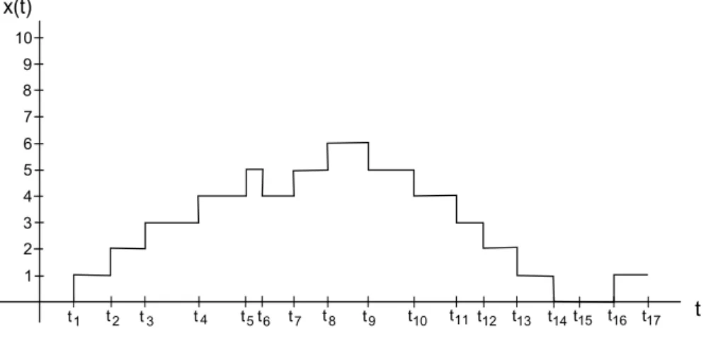
and “𝑑”. For example, considering the warehouse initially empty, if the sequence of events which occurred in the system is:
𝑎𝑎𝑎𝑎𝑎𝑑𝑑𝑑𝑎𝑎𝑎𝑑𝑑𝑎
the number of boxes in the warehouse will be equal to four.
Input
a d
Output
Figure 2.1: Warehouse System
Another example of system evolution is presented in Figure2.2. By this figure, it is possible to see that five events “𝑎” occur , at dates 𝑡1 to 𝑡5, and in sequence
one event “𝑑” occurs at date 𝑡6 and so on.
Therefore, this system is an event-driven system and the set of possible reached states is discrete.
x(t)
t 1
2 3 4 5 6 7 8 9 10
t1 t2 t3 t4 t5 6t t7 t8 t9 t10 t11t12 t13 t14 15t t16 t17
There are some tools to deal with DEDS, for example, Graphs, Automata, Petri Nets, Timed Event Graphs, Markov Process and Dioid Algebra. In this thesis, the methodologies will be develop based on Graphs, Petri Nets, Timed Event Graphs and systems described by using Dioid Algebra.
2.2
Graphs
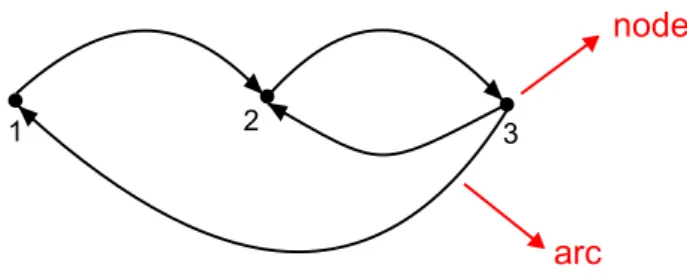
In this section, some necessary graph concepts for the comprehension of this thesis are presented. Concepts such as the definition of a graph and connected graphs are useful to understand the Petri nets and some tools in max-plus algebra. The definitions were obtained in Baccelli et al. (1992). Firstly, the directed graphs are defined.
Definition 2.2.1 (Directed Graph) A directed graph 𝐺 is a pair(𝑉, 𝜖), being
𝑉 a set of elements called nodes and 𝜖 a set of elements which are ordered pairs of nodes, called arcs.
A directed graph is illustrated in Figure 2.3.
1 2 3
node
arc
Figure 2.3: Directed Graph
Definition 2.2.3 (Path, Circuit, Loop, Length) A path 𝜌 is a sequence of nodes 𝑖1, 𝑖2, ..., 𝑖𝑝, 𝑝 > 1, so that 𝑖𝑗 belongs to the set of nodes 𝜋(𝑖𝑗+1), 𝑗 =
1,..., 𝑝−1, in which the set 𝜋(𝑖𝑗+1) indicates the predecessor nodes of node 𝑖𝑗+1.
Node 𝑖1 is the initial node and node 𝑖𝑝 is the final node of the path. In other
words, a path is a sequence of arcs which connects a sequence of nodes. When the initial node and the final node are the same, it is called the path as a circuit, by definition a circuit is defined as a sequence of nodes (𝑖1, 𝑖2, ...,𝑖𝑝, 𝑖1). A loop
is a circuit(𝑖,𝑖)composed by a single node which is the initial and the final node.
The length of a path or a circuit is equal to the sum of the lengths of the arcs which compose this path. The lengths of the arcs are1 unless otherwise specified. By this definition, the length of a loop is 1.
Definition 2.2.4 (Subgraphs) Given a graph 𝐺= (𝑉, 𝜖), a graph 𝐺′ = (𝑉′, 𝜖′)
is said to be a subgraph of 𝐺 if 𝑉′ ⊂ 𝑉 and if 𝜖′ consists of a set of arcs of 𝐺
which have their origins and destinations in 𝑉′.
Definition 2.2.5 (Connected Graphs) A graph is called connected when there exists a chain joining 𝑖 and 𝑗 for every pair of nodes 𝑖 and 𝑗. A chain is a se-quence of nodes (𝑖1, 𝑖2, ..., 𝑖𝑝) so that between each pair of successive nodes either
the arc (𝑖𝑗, 𝑖𝑗+1) or the arc (𝑖𝑗+1, 𝑖𝑗) exists. If one disregards the directions of the
arcs in the definition of a path, one obtains a chain.
Definition 2.2.6 (Strongly Connected Graphs) A graph is called strongly connected when there is at least a path from 𝑖 to 𝑗 for any two different nodes 𝑖
and 𝑗 . According to this definition, a graph which is comprised by an isolated node, with or without a loop, is a strongly connected graph.
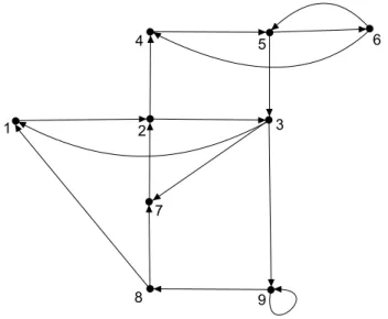
concepts introduced in this section. It is a directed graph since the arcs are di-rected. The graph has nine nodes. Node 2 is a predecessor node of node 3, therefore 2∈𝜋(3). The sequence of nodes 1, 2, 3, 7, 2, 4is a path. The arc(9,9)
is a loop. The sequence of nodes 1, 2, 3, 9, 8, 1 is a circuit of length equal to 5. The graph of Figure 2.4 is connected.
1 2 3
4 5 6
7
8 9
Figure 2.4: Example of Directed Graph
Definition 2.2.7 (Bipartite Graph) If the set of nodes 𝑉 of a graph𝐺 can be partitioned into two disjoint subsets 𝑉1 and 𝑉2 so that, every arc of 𝐺 connects
an element of 𝑉1 to one of 𝑉2 or the other way around, then𝐺 is called bipartite.
Definition 2.2.8 (Equivalence Relation R) Let 𝑖, 𝑗 ∈ 𝑉 be two nodes of a
graph. The equivalence 𝑖 R 𝑗 holds, if either 𝑖=𝑗 or there exist paths from 𝑖 to
𝑗 and from 𝑗 to 𝑖.
Definition 2.2.9 (Maximal Strongly Connected Subgraphs) The subgraphs
𝐺𝑖 = (𝑉𝑖, 𝜖𝑖) corresponding to the equivalence classes determined by R are the
Definition 2.2.10 (Cycle Mean) (Baccelli et al., 1992) The mean weight of a path is defined as the sum of the weights of the individual arcs of this path, divided by the length of this path. If the path is denoted 𝜌, then the mean weight is equal to |𝜌|𝑤/|𝜌|𝑙 (where |𝜌|𝑤 is the weight of path 𝜌 and |𝜌|𝑙 is the length of
path 𝜌). If such path is a circuit, one talks about the mean weight of circuit, or simple cycle mean.
Definition 2.2.11 (Maximum Cycle Mean) The maximum cycle mean is taken over all circuits in the graph, i.e., the maximum over all the cycle mean.
These definitions are useful to understand and work with Petri nets theory since these nets are directed graphs.
2.3
Petri Nets
Petri nets are directed bipartite graphs, more precisely, a Petri net is a weighted graph endowed with a finite set of places, transitions and arcs. Besides that, there are arc weight functions.
Definition 2.3.1 (Petri Nets) (Baccelli et al., 1992) A Petri net is a directed bipartite graph (𝑃, 𝑇, 𝐴, 𝑤), being 𝑃 a finite set of places, 𝑇 a finite set of tran-sitions, 𝐴 a finite set of arcs, and 𝑤 are arc weight functions.
In this thesis, only connected graphs are stated and treated, i.e., there are no isolated places in the graph. Consider the graph in Figure2.5 to illustrate Petri nets.
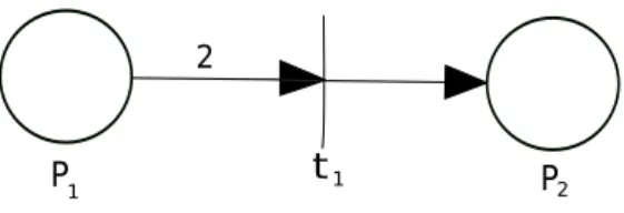
The net can be defined by the set 𝑃 = {𝑃1, 𝑃2}, the set 𝑇 = {𝑡1}, the set
2
P1 t1 P2
Figure 2.5: Petri Net
Definition 2.3.2 (Input and Output Places) Considering an arc(𝑃𝑖, 𝑡𝑖), the
place𝑃𝑖 is called input place for transition 𝑡𝑖 and𝑡𝑖 is called output transition for
place 𝑃𝑖, represented by 𝐼(𝑡𝑖) and 𝑂(𝑃𝑖), respectively. In the same way,
consid-ering an arc (𝑡𝑗, 𝑃𝑗), the place 𝑃𝑗 is called output place for transition𝑡𝑗 and 𝑡𝑗 is
called input place for place 𝑃𝑗, represented by 𝑂(𝑡𝑗) and 𝐼(𝑃𝑗).
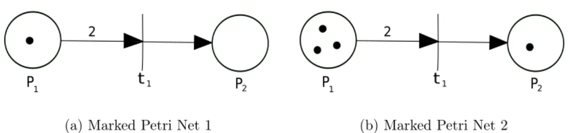
Definition 2.3.3 (Marked Petri Nets) (Cassandras and Lafortune, 2008) A marked Petri net is a quintuple (𝑃, 𝑇, 𝐴, 𝑤, 𝑥), in which (𝑃, 𝑇, 𝐴, 𝑤) is a Petri
net and 𝑥 is a marking of the set of places. The vector
𝑥=[︁ 𝑥(𝑝1) 𝑥(𝑝2) · · · 𝑥(𝑝𝑛)
]︁
∈N𝑛
is a row vector associated with 𝑥.
Considering the Petri net in Figure 2.5, there are a lot of possible markings for this net, one of them is the vector
𝑥1 = [︁
1 0
]︁
and another vector is
𝑥2 = [︁
3 1
]︁
.
2
P1 t1 P2
(a) Marked Petri Net 1
2
P1 t1 P2
(b) Marked Petri Net 2
Figure 2.6: Marked Petri Nets. (a) Marked Petri Net with vector x1. (b)Marked Petri Net
with vectorx2.
The markings in each place (black circles) are called tokens. The way how a net is marked represents the net state because there is only one marking for each state reached by the net. In order to simplify the nomenclature, the marked Petri nets will be called just Petri nets, since all Petri nets are marked, even if the marking is a null marking.
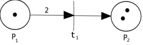
Definition 2.3.4 (Enabled Transition) (Cassandras and Lafortune, 2008) A transition 𝑡𝑗 ∈𝑇 in a Petri net is called enabled if
𝑥(𝑝𝑖)⪰𝑤(𝑝𝑖,𝑡𝑗) for all 𝑝𝑖 ∈𝐼(𝑡𝑗)
being𝐼(𝑡𝑗) the set of input places of transition 𝑡𝑗.
Definition 2.3.5 (Dynamic of Petri Net) (Cassandras and Lafortune,2008) The state transition function 𝑓 : N𝑛 ×𝑇 → N𝑛, of a Petri net (𝑃,𝑇,𝐴,𝑤,𝑥) is
defined for the transition 𝑡𝑗 ∈𝑇 if and only if,
𝑥(𝑝𝑖)⪰𝑤(𝑝𝑖,𝑡𝑗), for all 𝑝𝑖 ∈𝐼(𝑡𝑗)
being 𝐼(𝑡𝑗) the set of input places of a transition 𝑡𝑗. If 𝑓(𝑥,𝑡𝑗) is defined, it is
defined 𝑥+=𝑓(𝑥,𝑡
𝑗), in which
𝑥+(𝑝𝑖) =𝑥(𝑝𝑖)−𝑤(𝑝𝑖,𝑡𝑗) +𝑤(𝑡𝑗,𝑝𝑖), 𝑖= 1,...,𝑛. (2.1)
For example, in Figure2.6a, the transition𝑡1 is not enabled and in Figure2.6b
the transition 𝑡1 is enabled. When the transition 𝑡1 fires, from Figure 2.6b, two
tokens are removed from place 𝑃1 and one token is placed in 𝑃2, in accordance
with the weights of the arcs. The obtained Petri net when the transition𝑡1 fires,
from marking 𝑥2, is shown in Figure 2.7. Therefore, it possible to conclude that
the number of tokens in a net is not conserved for some models.
2
P1 t1 P2
Figure 2.7: Petri net when transition t1 fire from markingx2
The Equation 2.1 can be generalized by the following matrix equation:
𝑋+ =𝑋+𝑢𝐴 (2.2)
represented by number 1in vector 𝑢, otherwise it is represented by0. Only one transition fires each time) and matrix 𝐴 is the incidence matrix (the matrix A represents the number of tokens removed and placed in places by the transitions). A transition in a net can fire only if
𝑋+𝑢𝐴−⪰0 (2.3)
in which matrix 𝐴− represents the number of tokens taken off by transitions of
places. In order to illustrate these equations, consider the following example.
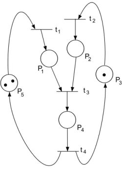
Example: 2.3.1 Consider the following graph in Figure 2.8. The incidence ma-trix is given by:
P
P
P
P P
1
2
3
4 5
t
t
t
t
1
2
3
4
𝐴 = ⎡ ⎢ ⎢ ⎢ ⎢ ⎢ ⎢ ⎢ ⎣
1 0 0 0 −1
0 1 −1 0 0
−1 −1 0 1 0
0 0 1 −1 1
⎤ ⎥ ⎥ ⎥ ⎥ ⎥ ⎥ ⎥ ⎦
The incidence matrix represents the graph structure and it can be obtained by looking for the weights between places and transitions. For example, consider the entry 𝑎𝑖𝑗 from matrix 𝐴, the variable 𝑖 is related to transitions and the variable
𝑗 is related to places. Therefore the entry𝑎11 is the weight between the transition
𝑡1 and place 𝑃1 and it is equal to 1 because 𝑡1 puts one token in place 𝑃1. The
entry 𝑎15 is equal to −1 because 𝑡1 removes one token from place 𝑃5, and so on.
The matrix𝐴− is obtained similarly to𝐴. The matrix 𝐴− is obtained from the
number of tokens that each transition removes from each place. In this example, the matrix 𝐴− is given by:
𝐴− =
⎡ ⎢ ⎢ ⎢ ⎢ ⎢ ⎢ ⎢ ⎣
0 0 0 0 −1
0 0 −1 0 0
−1 −1 0 0 0
0 0 0 −1 0
⎤ ⎥ ⎥ ⎥ ⎥ ⎥ ⎥ ⎥ ⎦ .
The initial marking of the net in this example is:
𝑋0 = [︁
𝑃1 𝑃2 𝑃3 𝑃4 𝑃5 ]︁
=[︁ 0 0 1 0 2
]︁
.
If the transition 𝑡2 will be fired, the vector 𝑢 can be given by:
𝑢=[︁ 0 1 0 0 ]︁,
but, it is necessary that
𝑋0+𝑢𝐴− ⪰0.
This inequality holds so the transition 𝑡2 is enabled to fire. If 𝑡2 fires the reached
state is given by:
𝑋1 =𝑋0 +𝑢𝐴,
𝑋1 = [︁
0 1 0 0 2
]︁
.
The Petri nets are useful to model Discrete Event Systems and the model can use processing time associated with its structure, called holding time. There are some ways to do the timing, being the time associated with places (Net P-timed) or the time associated with transitions (Net T-timed) the most common. The nets P-timed and T-timed are showed in Figure2.9aand Figure2.9b, respectively.
P1 t1 P2
4 1
(a) P-timed Petri Net
P1 t1 P2
3
(b) T-timed Petri Net
Figure 2.9: Timed Petri Nets. (a)P-timed Petri Net. (b)T-timed Petri Net.
contributing to the enabling of output transitions. In this thesis, the holding time is associated with places.
The Petri nets of interest for this thesis are a subclass called Timed Event Graphs (TEG), these nets are introduced in the next section.
2.3.1 Timed Event Graphs
Definition 2.3.6 (Event Graph) A Petri net is called an event graph if each place has at most one input transition 𝐼(𝑃𝑖) and at most one output transition
𝑂(𝑃𝑖).
An event graph is a Petri net in which each place has at most one input transition and at most one output transition. The event graph are able to model discrete event systems endowed with time delay and synchronization phenomena, i.e. the event graphs are not able to model systems where there is a competition for resources.
Definition 2.3.7 (Timed Event Graph (TEG)) (Baccelli et al.,1992) A timed event graph is an event graph in which each place has a holding time associated with it.
Assumption: 2.3.1 In this thesis, the time associated with places is assumed non-varying.
Figure 2.10 shows a TEG with three places (𝑃1, 𝑃2 and 𝑃3) and three
transi-tions(𝑢1, 𝑥1 and𝑥2). In this graph, the transition𝑥1can fire by𝑘𝑡ℎ date after the
𝑘𝑡ℎ firing date of transition 𝑢
1 and the (𝑘−1)𝑡ℎ firing date of transition 𝑥2. The
𝑘𝑡ℎ firing date of transition 𝑥
1 is related to the (𝑘−1)𝑡ℎ firing date of transition
P1 1 P2
P3
2
5
X X
u1
Figure 2.10: Timed-Event Graph.
𝑥1 and this token was placed in 𝑃3 when the transition 𝑥2 fired at the (𝑘−1)𝑡ℎ
date. Then, the transition 𝑥1 will be enabled to fire at the 𝑘𝑡ℎ date after the
greatest date between the firing date 𝑢(𝑘) and 𝑥2(𝑘 −1). The place 𝑃2 has 5
time units associated with it, therefore when a token arrives at this place it must wait, at least, five time units before contributing to enabling transition 𝑥2. It is
possible to describe the 𝑘𝑡ℎ firing date of transition 𝑥
1 and 𝑥2 by the following
equations:
𝑥1(𝑘) = 𝑚𝑎𝑥{𝑢1(𝑘), 𝑥2(𝑘−1)}, (2.4)
𝑥2(𝑘) =𝑥1(𝑘) + 5. (2.5)
The Equations 2.4 and 2.5 use the operator addition and the operator max-imization. The operator addition can be related with time delay linked with places. The operator maximization can be related to the synchronization phe-nomena. With these operators the TEG dynamics can be completely described. Those equations can be described using a dioid, which is an algebraic structure endowed with all properties of a ring, except the inverse additive element, so the dioids are characterized algebraically as an idempotent semiring (Baccelli et al.,
2.4
Dioids and Max-Plus Algebra
A ring is defined algebraically as (𝒜,⊕,⊗), with the set 𝒜 endowed with two internal operators. The operator ⊕ (addition) is associative, invertible, com-mutative and it has the neutral element 𝜀. The operator ⊗ (multiplication) is associative, commutative, it admits the neutral element𝑒 and, besides that, it is distributive with relation to⊕.
In this way, dioids are algebraic structures characterized as an idempotent semiring since the dioids have two operators and all properties of a ring, except the additive inverse element.
Definition 2.4.1 (Dioids) (Baccelli et al., 1992) A dioid is defined as a set 𝒟 endowed with two internal operators, ⊕ (addition) and ⊗ (multiplication), obeying the following axioms:
• The addition is associative and commutative: ∀𝑎,𝑏,𝑐 ∈ 𝒟, (𝑎 ⊕𝑏)⊕ 𝑐 =
𝑎⊕(𝑏⊕𝑐) =𝑐⊕(𝑏⊕𝑎).
• The multiplication is associative and distributive on left and on right with relation to addition: ∀𝑎,𝑏,𝑐∈ 𝒟, (𝑎⊗𝑏)⊗𝑐=𝑎⊗(𝑏⊗𝑐) and (𝑎⊕𝑏)⊗𝑐=
(𝑎⊗𝑐)(𝑏⊗𝑐).
• Existence and absorbing by neutral element of addition (𝜀): ∀𝑎 ∈ 𝒟,𝑎⊕𝜀=𝑎
and 𝑎⊗𝜀=𝜀.
• Existence of identity element of multiplication (𝑒): ∀𝑎∈ 𝒟, 𝑎⊗𝑒=𝑒⊗𝑎=𝑎. • Idempotency of addition: ∀𝑎∈D, 𝑎⊕𝑎=𝑎.
and if, besides that, it is closed in relation to infinite sums and the multiplication is distributive with relation to infinite sums.
2.4.1 Lattice Properties of Dioids
The properties and definitions presented in this subsection are used in this thesis and they were obtained inBaccelli et al. (1992).
Order Relation: a binary relation (denoted by ⪰) which is reflexive, transi-tive and anti-symmetric.
Total (Partial) Order: the order is total if for each pair of elements (𝑎,𝑏),
the order relation holds true either for(𝑎,𝑏) or for (𝑏,𝑎), or otherwise stated, if 𝑎
and 𝑏 are always comparable; otherwise, the order is partial.
Ordered Set: a set endowed with an order relation; it is sometimes useful to represent an ordered set by an undirected graph the nodes of which are the element of the set; two nodes are connected by an arc if the corresponding ele-ments are comparable, the greater one being higher in the diagram; the minimal number of arcs is represented, the other possible comparisons being derived by transitivity.
Top Element (of an ordered set): an element which is greater than any other element of the set.
Bottom Element (of an ordered set): an element which is smaller than any other element of the set.
Maximum Element: an element of the subset which is greater than any other element of the subset; if it exists, it is unique; it coincides with the top element if the subset is equal to the whole set.
other element of the subset; if it exists, it is unique; it coincides with the bottom element if the subset is equal to the whole set.
Maximal Element: an element of the subset which is not smaller than any other element of the subset; if a subset has a maximum element, it is the unique maximal element.
Majorant: an element not necessarily belonging to the subset which is greater than any other element of the subset; if a majorant belongs to the subset, it is the maximum element.
Minorant: an element not necessarily belonging to the subset which is smaller than any other element of the subset; if a minorant belongs to the subset, it is the minimum element.
Upper Bound: the least majorant, that is, the minimum element of the subset of majorants.
Lower Bound: the greatest minorant, that is, the maximum element of the subset of minorants.
2.4.2 Max-Plus Algebra
The max-plus algebra is defined as a complete dioid endowed with the structure
(Z∪ {−∞}, 𝑚𝑎𝑥, +), being denoted by Z𝑚𝑎𝑥.
Definition 2.4.2 (Algebraic Structure of Z𝑚𝑎𝑥) The symbolZ𝑚𝑎𝑥 denotes the
set(Z∪ {−∞}endowed with the maximization operation and the addition opera-tion represented, respectively, as⊕ and⊗, and the convention (−∞)+∞=−∞.
The Kleene star operation is another operation defined on any dioid, denoted by the symbol*. This operator is algebraically defined as:
𝑎* =⨁︀
being 𝑎0 =𝑒.
In subsection 2.3.1, the dynamic behavior of a TEG could be completely de-scribed using only two operators: the addition operator and the maximization operator. Then, the TEG can be completely described, in a linear way, using the max-plus algebra, i.e., it is possible to rewrite Equations 2.4 and 2.5 using the max-plus algebra as:
𝑥1(𝑘) =𝑢1(𝑘)⊕𝑥2(𝑘−1) (2.6)
and
𝑥2(𝑘) = 5⊗𝑥1(𝑘). (2.7)
In this thesis, in order to simplify the notation, the symbol ⊗will be omitted in equations when convenient, without any information loss. From TEG of Figure
2.10, the output dates will be given by:
𝑦(𝑘) =𝑥2(𝑘). (2.8)
By Equations 2.6, 2.7 and 2.8, it is possible to rewrite these equations in matrix notation as state space equations in max-plus algebra:
⎧
⎨
⎩
𝑥(𝑘) = 𝐴𝑥(𝑘−1)⊕𝐵𝑢(𝑘)
𝑦(𝑘) = 𝐶𝑥(𝑘).
(2.9)
in which𝐴,𝐵and𝐶are matrix of appropriate dimensions with the characteristics of the system, 𝑥(𝑘) the state vector (also called internal) at 𝑘𝑡ℎ date, 𝑢(𝑘) the
2.4.3 Graphs and Matrices
An important tool to deal with TEG described by max-plus algebra are the matrices in Z𝑚𝑎𝑥. All weighted graphs (graphs in which the arcs are associated
with weights) are related with matrices (Baccelli et al.,1992),i.e., every weighted graph has a representative matrix, besides that, every matrix whose entries are integers has a representative graph.
The matrix operations in max-plus algebra are similar to the matrix operations in conventional algebra. Let𝐴, 𝐵 ∈Z¯𝑛×𝑚
𝑚𝑎𝑥, being𝑛,𝑚∈N, the addition operation
is defined as:
[𝐴⊕𝐵] =𝑎𝑖𝑗 ⊕𝑏𝑖𝑗 (2.10)
in which 𝑖 and 𝑗 are, respectively, the rows and columns of matrices 𝐴 and 𝐵. Let 𝐶 ∈ Z¯𝑚×𝑝
𝑚𝑎𝑥, the matrix multiplication between matrix 𝐴 and matrix 𝐶 in
Z𝑚𝑎𝑥 is defined as:
[𝐴⊗𝐶]𝑖𝑘 =
𝑚
⨁︁
𝑗=1
𝑎𝑖𝑗 ⊗𝑐𝑗𝑘 (2.11)
in which 𝑖 and 𝑘 are, respectively, the row and column indexes of the elements in the resulting matrix.
Example: 2.4.1 (Representation and Operations with Matrices) Consider the graphs of Figure 2.11. The graph A, graph B and graph C can be related to the matrices 𝐴, 𝐵 and 𝐶, respectively given by:
𝐴=
⎡
⎣
4 3
5 2
⎤
⎦, 𝐵 = ⎡
⎣
2 6
1 3
⎤
3 5 2 4 2 1
(a) Graph A -G(A)
6 1 3 2 2 1
(b) Graph B -G(B)
0 1 4 1 2 1
(c) Graph C -G(C)
Figure 2.11: Weighted Graphs. (a)Graph A.(b)Graph B.(c)Graph C.
and 𝐶= ⎡ ⎣ 1 0 1 4 ⎤ ⎦. Then
𝐴⊕𝐵 =
⎡
⎣
4⊕2 3⊕6
5⊕1 2⊕3
⎤ ⎦= ⎡ ⎣ 4 6 5 3 ⎤ ⎦ and
(𝐴⊕𝐵)⊗𝐶=
⎡
⎣
4⊗1⊕6⊗1 4⊗0⊕6⊗4
5⊗1⊕3⊗1 5⊗0⊕3⊗4
⎤
⎦= ⎡
⎣
5⊕7 4⊕10
6⊕4 5⊕7
⎤ ⎦= ⎡ ⎣ 7 10 6 7 ⎤ ⎦.
InZ𝑚𝑎𝑥 the identity matrix is denoted by 𝐼 with 𝑖𝑚𝑛 =𝑒 for 𝑚=𝑛 and 𝑖𝑚𝑛=𝜀
for𝑚 ̸=𝑛. Let 𝐴∈R¯𝑚×𝑚
𝑚𝑎𝑥 , the Kleene star operator is defined for matrices as:
𝐴* =⨁︀
𝑚∈N𝐴𝑚,
in which𝐴𝑚=𝐴⊗𝐴𝑚−1 and 𝐴0 =𝐼.
will be denoted by a dot in matrix notation.
Example: 2.4.2 (Timed Event Graph and Max-Plus Algebra) In order to illustrate the linearity features of the dynamic behavior of the systems by max-plus algebra, consider the following timed event graph in Figure 2.12:
t t t t
t
u x x x x
1
1 1
2
2
3 4
5
3 4
u2
Figure 2.12: Timed Event Graph
The TEG in Figure2.12can model a queuing system, a manufacturing system, and so forth. As explained in Chapter 1, the dynamic behavior of a TEG can be described using only the maximization operator (𝑚𝑎𝑥) and the addition operator (+) in conventional algebra, by the following equations:
𝑥1(𝑘) =𝑚𝑎𝑥(𝑡1+𝑢1(𝑘), 𝑥2(𝑘−1)) (2.12)
𝑥2(𝑘) =𝑡2+𝑚𝑎𝑥(𝑡1+𝑢1(𝑘), 𝑥2(𝑘−1)) (2.13)
𝑥3(𝑘) =𝑚𝑎𝑥(𝑡3+𝑡2+𝑚𝑎𝑥(𝑡1 +𝑢1, 𝑥2(𝑘−1)), 𝑡5+𝑢2(𝑘), 𝑥4(𝑘−1)) (2.14)
𝑥4(𝑘) =𝑡4+𝑚𝑎𝑥(𝑡3+𝑡2+𝑚𝑎𝑥(𝑡1+𝑢1(𝑘), 𝑥2(𝑘−1)),𝑡5+𝑢2(𝑘), 𝑥4(𝑘−1))
(2.15) The Equations 2.12 to 2.15 are complex nonlinear equations in conventional algebra that can be used to describe the dynamic behavior of the system. In addi-tion, these equations are obscure from the point of view of conventional algebra.
using the max-plus algebra, in which the maximization is denoted by ⊕ and the addition denoted by ⊗ (the symbol ⊗ will be omitted by convenience), by the following equations:
𝑥1(𝑘) = 𝑥2(𝑘−1)⊕𝑡1𝑢1(𝑘) (2.16)
𝑥2(𝑘) = 𝑡2𝑥2(𝑘−1)⊕𝑡2𝑡1𝑢1(𝑘) (2.17)
𝑥3(𝑘) = 𝑡2𝑡3𝑥2(𝑘−1)⊕𝑥4(𝑘−1)⊕𝑡3𝑡2𝑡1𝑢1(𝑘)⊕𝑡5𝑢2(𝑘) (2.18)
𝑥4(𝑘) = 𝑡4𝑡3𝑡2𝑥2(𝑘−1)⊕𝑡4𝑥4(𝑘−1)⊕𝑡4𝑡3𝑡2𝑡1𝑢1(𝑘)⊕𝑡5𝑡4𝑢2(𝑘) (2.19)
The Equations 2.16 to 2.19 are linear in max-plus algebra and they can be written in matrix notation as:
⎡ ⎢ ⎢ ⎢ ⎢ ⎢ ⎢ ⎢ ⎣
𝑥1(𝑘)
𝑥2(𝑘)
𝑥3(𝑘)
𝑥4(𝑘) ⎤ ⎥ ⎥ ⎥ ⎥ ⎥ ⎥ ⎥ ⎦ = ⎡ ⎢ ⎢ ⎢ ⎢ ⎢ ⎢ ⎢ ⎣
. 𝑒 . . . 𝑡2 . .
. 𝑡3𝑡2 . 𝑒
. 𝑡4𝑡3𝑡2 . 𝑡4 ⎤ ⎥ ⎥ ⎥ ⎥ ⎥ ⎥ ⎥ ⎦ ⎡ ⎢ ⎢ ⎢ ⎢ ⎢ ⎢ ⎢ ⎣
𝑥1(𝑘−1)
𝑥2(𝑘−1)
𝑥3(𝑘−1)
𝑥4(𝑘−1) ⎤ ⎥ ⎥ ⎥ ⎥ ⎥ ⎥ ⎥ ⎦ ⊕ ⎡ ⎢ ⎢ ⎢ ⎢ ⎢ ⎢ ⎢ ⎣
𝑡1 .
𝑡2𝑡1 .
𝑡3𝑡2𝑡1 𝑡5
𝑡4𝑡3𝑡2𝑡1 𝑡5𝑡4 ⎤ ⎥ ⎥ ⎥ ⎥ ⎥ ⎥ ⎥ ⎦ ⎡ ⎣
𝑢1(𝑘)
𝑢2(𝑘) ⎤
⎦
in which the dot in matrices is the neutral element of addition 𝜀.
2.4.4 Systems of Linear Equations
In this subsection, some systems of linear equations are addressed, mainly in matrix notation. Dealing with max-plus algebra, the general system of equations is
𝐴𝑥⊕𝑐=𝐶𝑥⊕𝑑 (2.20)
in which𝐴and𝐵 are matrices and𝑐and𝑑are vectors of appropriate dimensions.
Definition 2.4.3 (Canonical form of a System of Affine Equations) (Baccelli et al., 1992) The system 𝐴𝑥⊕𝑐= 𝐵𝑥⊕𝑑 is said to be in canonical form if 𝐴,
𝐵, 𝑐and 𝑑 satisfy:
• 𝐵𝑖𝑗 =𝜀 if 𝐴𝑖𝑗 ≻𝐵𝑖𝑗, and 𝐴𝑖𝑗 =𝜀 if 𝐴𝑖𝑗 ≺𝐵𝑖𝑗;
• 𝑑𝑖 =𝜀 if 𝑏𝑖 ≻𝑑𝑖, and 𝑏𝑖 =𝜀 and 𝑏𝑖 ≺𝑑𝑖.
Cuninghame-Green and Butkovic(2003) developed a methodology to find the greatest solution, smaller than the initial condition for Equation2.20. Therefore, considering the initial condition equal to ⊤ (the greatest element in max-plus algebra), the method finds the greatest solution to that equation. The solution to Equation 2.20 will be better discussed in Subsection 2.7.1.
For instance, there are two classes of linear systems of interest for which there exists a satisfactory theory. The first one is𝑥=𝐴𝑥⊕𝑏.
The (𝐴*)
𝑖𝑗 represents the maximum weight of all paths of any length from 𝑗
to𝑖 in a graph. Thus, the necessary and sufficient condition for the existence of
(𝐴*)
𝑖𝑗 is the non existence of circuits with positive weight.
Theorem 2.4.2 (Baccelli et al., 1992) If a graph has no circuit with positive weight, then
𝐴* =𝑒⊕𝐴⊕. . .⊕𝐴𝑛−1 (2.21) where 𝑛 is the dimension of matrix 𝐴.
The second class of linear systems is𝐴𝑥=𝑏. In this case, however, the notion of subsolution of 𝐴𝑥 =𝑏 must be considered, i.e., the values of 𝑥 which satisfy
𝐴𝑥⪯𝑏, where the order relation on the vectors is defined by 𝑥⪯𝑦 if 𝑥⊕𝑦=𝑦.
Theorem 2.4.3 (Baccelli et al.,1992) Given an𝑛×𝑛matrix 𝐴and an n-vector
𝑏 in Z𝑚𝑎𝑥, the greatest solution of 𝐴𝑥⪯𝑏 exists and it is given by
−𝑥𝑗 = max
𝑖 (−𝑏𝑖+𝐴𝑖𝑗) (2.22)
or
𝑥𝑗 = min
𝑖 (𝑏𝑖−𝐴𝑖𝑗) (2.23)
The solution to equation𝐴𝑥=𝑏and the notion of subsolution will be discussed in Section 2.5.
2.4.5 Spectral Theory of Matrices
through node𝑖of𝐺can be written as(𝐴𝑗)
𝑖𝑖. The maximum of these weights over
all nodes is ⨁︀𝑛
𝑖=1(𝐴𝑗)𝑖𝑖, that can be written as the trace of matrix𝐴. Then, the
maximum cycle mean (𝜈) of a graph can be given, in max-plus algebra notation, by:
𝜈=
𝑛
⨁︁
𝑗=1
(trace(𝐴𝑗))1/𝑗 (2.24)
Definition 2.4.4 (Baccelli et al., 1992) Let 𝐴∈Z𝑚𝑎𝑥 a square matrix. If there
exists a scalar 𝜆∈Z𝑚𝑎𝑥 and a vector 𝑣 ∈Z𝑚𝑎𝑥 that has at least one finite entry
so that
𝐴⊗𝑣 =𝜆⊗𝑣, (2.25)
then𝜆is called an eigenvalue of𝐴and𝑣 an eigenvector associated with eigenvalue
𝜆.
Theorem 2.4.4 (Baccelli et al., 1992) The necessary and sufficient condition for a square matrix 𝐴 to be irreducible is the graph 𝐺(𝐴) associated with matrix
𝐴 be strongly connected.
Theorem 2.4.5 (Baccelli et al.,1992) If𝐴is irreducible, or equivalently if 𝐺(𝐴)
is strongly connected, there exists one and only one eigenvalue (but possible sev-eral eigenvectors). This eigenvalue is equal to the maximum cycle mean of the graph:
𝜆= max
𝜁
|𝜁|𝑤
|𝜁|𝑙
(2.26)
where 𝜁 ranges over the set of circuits of 𝐺(𝐴), in which |𝜁|𝑤 is the weight of
2.4.6 Asymptotic Behavior of 𝐴𝑘
Definition 2.4.5 (Critical Circuits) (Baccelli et al., 1992) A circuit 𝜁 of the graph 𝐺(𝐴) is called critical if it has maximum weight, that is, |𝜁|𝑤 =𝑒.
Definition 2.4.6 (Critical Graph) (Baccelli et al., 1992) The critical graph
𝐺𝑐(𝐴) consists of those nodes and arcs of𝐺(𝐴) which belong to a critical circuit
of 𝐺(𝐴). Its nodes constitute the set 𝑉𝑐.
Example: 2.4.3 Baccelli et al. (1992) Consider the matrix
𝐴= ⎡ ⎢ ⎢ ⎢ ⎢ ⎢ ⎢ ⎢ ⎣
𝑒 𝑒 𝜀 𝜀
−1 −2 𝜀 𝜀 𝜀 −1 −1 𝜀 𝜀 𝜀 𝑒 𝑒
⎤ ⎥ ⎥ ⎥ ⎥ ⎥ ⎥ ⎥ ⎦ .
Its precedence graph 𝐺(𝐴) has three critical circuits, namely: the circuit from node 1to node 1, the circuit from node3 to node4 and to node 3 and the circuit from node 4 to node 4.
Its critical graph is the precedence graph of matrix
𝐶 = ⎡ ⎢ ⎢ ⎢ ⎢ ⎢ ⎢ ⎢ ⎣
𝑒 𝜀 𝜀 𝜀 𝜀 𝜀 𝜀 𝜀 𝜀 𝜀 𝜀 𝜀 𝜀 𝜀 𝑒 𝑒
⎤ ⎥ ⎥ ⎥ ⎥ ⎥ ⎥ ⎥ ⎦ .
Finally, the matrix 𝐴 has the eigenvector
[︁
𝑒 −1 −2 −2
associated with eigenvalue 𝑒.
Definition 2.4.7 (Baccelli et al., 1992) The cyclicity of a maximal strongly con-nected subgraph is the greatest common divisor of the lengths of all its circuits. The cyclicity 𝜍(𝐺)of a graph 𝐺(𝐴) is the least common multiple of the cyclicities of all its maximal strongly connected subgraphs.
Definition 2.4.8 (Baccelli et al., 1992) Let 𝐴∈Z𝑚𝑎𝑥 such that the
correspond-ing graph has at least one circuit. The cyclicity of 𝐴, denoted by 𝜍(𝐴), is the cyclicity of the critical graph of 𝐴.
Theorem 2.4.6 (Baccelli et al., 1992) Let𝐴∈Z𝑚𝑎𝑥 an irreducible matrix, then
∃𝑘0 ∈ N such that ∀𝑘 ⪰ 𝑘0 : 𝐴𝑘+𝜍 = 𝜆𝜍 ⊗𝐴𝑘, in which 𝜆 is the eigenvalue of
matrix 𝐴 and 𝜍 is the cyclicity of 𝐴.
Definition 2.4.9 (Baccelli et al., 1992) A matrix 𝐴 is said to be cyclic if there exist 𝑑 and 𝑀 such that ∀𝑚 ⪰ 𝑀, 𝐴𝑚+𝑑 = 𝐴𝑚. The least such 𝑑 is called the
cyclicity of matrix 𝐴 and 𝐴 is said to be 𝑑−cyclic.
Lemma 2.4.1 (Baccelli et al., 1992) Let 𝐴 ∈ Z𝑚𝑎𝑥 be an irreducible matrix
endowed with cyclicity 𝜍(𝐴). Then, the cyclicity of matrix 𝐴𝜍 is equal to 1.
The cyclicity equal to 1 defines a periodic behavior in steady state. Consider the initial state 𝑥(0), from the state 𝑥(𝑘) at the 𝑘𝑡ℎ date, the behavior will be
periodic at𝑥(𝑘+𝜍), by the following equation:
𝑥(𝑘+𝜍) = 𝐴(𝑘+𝜍)⊗𝑥(0) (2.27)
that can be rewritten as
and considering, thanks to the periodicity,𝑥(𝑘) =𝐴𝑘𝑥(0),
𝑥(𝑘+𝜍) = 𝜆𝜍⊗𝑥(𝑘). (2.29)
For a graph endowed with cyclicity equal to 1, it is possible to show that
𝑥(𝑘+ 1) =𝐴⊗𝑥(𝑘) =𝜆𝑥(𝑘). (2.30)
Theorem 2.4.7 (Baccelli et al., 1992) A necessary and sufficient condition to have 𝑙𝑖𝑚𝑘→∞𝐴𝑘 = 𝑄 is that the cyclicity of each maximal strongly connected
subgraph of 𝐺(𝐴) is equal to 1.
Theorem 2.4.8 (Baccelli et al., 1992) Suppose that 𝐺(𝐴) is strongly connected graph. Then there exists a 𝑘′ such that
∀𝑘 ⪰𝑘′, 𝐴𝑘 =𝑄, (2.31)
if and only if the cyclicity of each maximal strongly connected subgraph of 𝐺(𝐴)
is equal to 1.
2.4.7 Max-Plus Linear Systems Theory Firstly, the max-plus linear systems are defined.
Definition 2.4.10 (Max-Plus Linear Dynamic Systems) The systems mod-eled by timed event graphs whose dynamics are described by max-plus algebra by state space equations are called Max-Plus Linear Dynamic Systems.
𝑥(𝑘)⪰𝑥(𝑘−1).
By using the max-plus algebra to describe max-plus linear systems it is com-mon to find equations such as
𝑥(𝑘) = 𝐴0𝑥(𝑘)⊕𝐴1𝑥(𝑘−1)⊕𝐵0𝑢(𝑘) (2.32)
in which𝐴0,𝐴1 and 𝐵0 are system matrices, but this equation can be rewritten
as:
𝑥(𝑘) =𝐴𝑥(𝑘−1)⊕𝐵𝑢(𝑘) (2.33) considering what was presented in Theorem2.4.1.
u P1 x1 P2 x2
P3
5 8
x3 3
Figure 2.13: Timed Event Graph
This important result can be better understood by considering the TEG in Figure 2.13, that has the firing dates described by an equation as Equation2.32, which can be rewritten as
in which𝑊 =𝐴1𝑥(𝑘−1)⊕𝐵0𝑢(𝑘). Suppose that𝑥(𝑘)is a solution, consequently,
𝑥(𝑘) must satisfy the Equation2.34, so
𝑥(𝑘) = 𝐴0𝑥(𝑘)⊕𝑊 (2.35)
𝑥(𝑘) = 𝐴0(𝐴0𝑥(𝑘)⊕𝑊)⊕𝑊 (2.36)
𝑥(𝑘) = 𝐴20𝑥(𝑘)⊕𝐴0𝑊 ⊕𝑊 (2.37)
...
𝑥(𝑘) = 𝐴𝑙
0𝑥(𝑘)⊕𝐴𝑙0−1𝑊 ⊕𝐴𝑙0−2𝑊 ⊕ · · · ⊕𝑊 (2.38)
and then 𝑥(𝑘) ⪰ 𝐴*
0𝑊. Equation 2.38 can be rewritten as 𝑥 = 𝐴𝑥⊕𝑏. Using
Theorem 2.4.1 and considering all graph circuits with non positive weights, the solution to Equation2.38 is given by:
𝑥(𝑘) = 𝐴*0𝑊, (2.39)
since the entries of 𝐴𝑙
0 are the maximum weights of circuits with weight 𝑙. For 𝑙
great enough, the entries of𝐴𝑙
0 are weights of the paths of length 𝑘. Those paths
necessarily traverse some circuits of 𝐴0 a number of times going to ∞ with 𝑙.
Since the weights of these circuits are all negative,𝐴𝑙
0 →[𝜀]when 𝑙 → ∞.
Replacing 𝑊 in Equation 2.39, the equation
𝑥(𝑘) =𝐴*0𝐴1𝑥(𝑘−1)⊕𝐴*0𝐵0𝑢(𝑘) (2.40)
is obtained, resulting in
with 𝐴=𝐴*
0𝐴1 and 𝐵 =𝐴*0𝐵0.
Example: 2.4.4 (Max-Plus Linear System) Consider a system modeled as the TEG in Figure 2.13. The dinamic behavior of the TEG can be described by the following equations in max-plus algebra:
𝑥1(𝑘) = 𝑥2(𝑘−1)⊕5⊗𝑢1(𝑘)
𝑥2(𝑘) = 8⊗𝑥1(𝑘)
𝑥3(𝑘) = 3⊗𝑥2(𝑘)
𝑦(𝑘) = 𝑥3(𝑘)
This equations can be rewritten as 𝑥(𝑘) =𝐴0𝑥(𝑘)⊕𝐴1𝑥(𝑘−1)⊕𝐵0𝑢(𝑘), in
matrix notation, as:
⎡ ⎢ ⎢ ⎢ ⎢ ⎣
𝑥1(𝑘)
𝑥2(𝑘)
𝑥3(𝑘) ⎤ ⎥ ⎥ ⎥ ⎥ ⎦ = ⎡ ⎢ ⎢ ⎢ ⎢ ⎣ . . .
8 . .
. 3 .
⎤ ⎥ ⎥ ⎥ ⎥ ⎦ ⎡ ⎢ ⎢ ⎢ ⎢ ⎣
𝑥1(𝑘)
𝑥2(𝑘)
𝑥3(𝑘) ⎤ ⎥ ⎥ ⎥ ⎥ ⎦ ⊕ ⎡ ⎢ ⎢ ⎢ ⎢ ⎣
. 𝑒 . . . . . . . ⎤ ⎥ ⎥ ⎥ ⎥ ⎦ ⎡ ⎢ ⎢ ⎢ ⎢ ⎣
𝑥1(𝑘−1)
𝑥2(𝑘−1)
𝑥3(𝑘−1) ⎤ ⎥ ⎥ ⎥ ⎥ ⎦ ⊕ ⎡ ⎢ ⎢ ⎢ ⎢ ⎣ 5 . . ⎤ ⎥ ⎥ ⎥ ⎥ ⎦
𝑢(𝑘)
(2.42)
𝑦(𝑘) = [︁ . . 𝑒 ]︁
⎡ ⎢ ⎢ ⎢ ⎢ ⎣
𝑥1(𝑘−1)
𝑥2(𝑘−1)
𝑥3(𝑘−1) ⎤ ⎥ ⎥ ⎥ ⎥ ⎦ . (2.43)
Using the previous result, the Equation 2.42 can be rewritten as the Equation
⎡ ⎢ ⎢ ⎢ ⎢ ⎣
𝑥1(𝑘)
𝑥2(𝑘)
𝑥3(𝑘) ⎤ ⎥ ⎥ ⎥ ⎥ ⎦ = ⎡ ⎢ ⎢ ⎢ ⎢ ⎣
. 𝑒 . . 8 . . 11 .
⎤ ⎥ ⎥ ⎥ ⎥ ⎦ ⎡ ⎢ ⎢ ⎢ ⎢ ⎣
𝑥1(𝑘−1)
𝑥2(𝑘−1)
𝑥3(𝑘−1) ⎤ ⎥ ⎥ ⎥ ⎥ ⎦ ⊕ ⎡ ⎢ ⎢ ⎢ ⎢ ⎣ 5 13 16 ⎤ ⎥ ⎥ ⎥ ⎥ ⎦
𝑢(𝑘). (2.44)
2.5
Residuation Theory
As previously mentioned, the max-plus algebra is an idempotent semiring (dioid) which does not have the inverse element for the ⊕ operation, therefore the op-eration⊕ is not particularly invertible for matrix applications such as finding a solution to matrix equations such as𝐴𝑥⪯𝑏 or𝐴𝑥=𝑏.
Definition 2.5.1 (Isotone Mappings) (Baccelli et al., 1992) A mapping 𝑓 de-fined on a dioid (𝒟,⊗,⊕) in a dioid (𝒞,⊗,⊕)is called isotone mapping if, for all
𝑎,𝑏∈ 𝒟, the following order relation is preserved:
𝑎⪯𝑏 ⇔𝑓(𝑎)⪯𝑓(𝑏)
The Residuation Theory, applied to dioids, deals with the inversion of isotone mappings and with the solutions to equations in partially ordered sets. Let 𝑓
be the isotone mapping of a dioid 𝒟 on a dioid 𝒞, if an equation 𝑓(𝑥) = 𝑏 is not surjective, the equation cannot have a solution to some values of 𝑏, and if
𝑓(𝑥) = 𝑏 is not injective, the equation has non unique solutions, i.e., equations like𝑓(𝑥) = 𝑏 can have innumerable or no solutions. The solution to this problem can be obtained considering a subset of solutions, i.e., values to 𝑥 that satisfy
𝑓(𝑥) ⪯ 𝑏. The Residuation Theory is particularly useful to find the maximal sub-solution to the inequality of the form 𝑓(𝑥) ⪯ 𝑏. The maximal sub-solution
to b. Dually, the Dual Residuation Theory finds the smallest super-solutions to equations such as𝑓(𝑥) =𝑏 in dioid algebra. The smallest super-solution 𝑥𝑠𝑢𝑝 is
the smallest solution to𝑥 such that 𝑓(𝑥𝑠𝑢𝑝) is greater than or equal to 𝑏 (Maia,
2003) (Baccelli et al., 1992). To ensure the existence of a lower bound and an upper bound, the dioids 𝒟 and 𝒞 are assumed as complete dioids.
The definitions and theorems presented below were obtained from Baccelli et al. (1992) and Maia (2003) and applications of Residuation Theory on dioids are shown in Baccelli et al. (1992).
Definition 2.5.2 (Residual and Residuated Mapping) Let𝒟and𝒞 be par-tially ordered sets. The isotone mapping 𝑓 : 𝒟 ↦→ 𝒞 is a residuated mapping if, for all 𝑦 ∈ 𝒞, there exists the greatest subsolution for the inequality 𝑓(𝑥) ⪯ 𝑦. The mapping 𝑓♯ is called residual of mapping 𝑓 and the greatest subsolution is
denoted by 𝑓♯(𝑦).
Theorem 2.5.1 (Residuation) Let 𝒟and𝒞 be ordered sets. The isotone map-ping 𝑓 : 𝒟 ↦→ 𝒞 is residuated, if and only if 𝑓♯ is the unique isotone mapping
such that
(𝑓 ∘𝑓♯)(𝑦)⪯𝑦 and (𝑓♯∘𝑓)(𝑥)⪰𝑥
∀𝑥∈ 𝒟 and ∀𝑦∈ 𝒞.
The residuated mappings to complete dioids are characterized by the following theorem.
𝑋 of 𝒟,
𝑓
(︃ ⨁︁
𝑥∈𝑋
𝑥
)︃
= ⨁︁
𝑥∈𝑋
𝑓(𝑥), 𝑓(𝜀) = 𝜀.
To dually residuated mappings, analogous statements from residuated map-pings can be demonstrated.
Definition 2.5.3 (Dual Residue and Dually Residuated Mapping) Let𝒟 and 𝒞 be ordered sets. The isotone mapping 𝑓 : 𝒟 ↦→ 𝒞 is dually residuated, if for all𝑦 ∈ 𝒞, there exists the smallest super-solution for the inequality 𝑓(𝑥)⪰𝑦. This smallest super-solution is denoted by𝑓♭(𝑦) and the mapping𝑓♭ is called dual
residue of 𝑓.
Theorem 2.5.3 (Dual Residuation) Let𝒟and𝒞 be ordered sets. The isotone mapping 𝑓 : 𝒟 ↦→ 𝒞 is dually residuated, if and only if, 𝑓♭ is the unique isotone
mapping such that,
𝑓 ∘𝑓♭(𝑦)⪰𝑦 and 𝑓♭∘𝑓(𝑥)⪯𝑥
∀𝑥∈ 𝒟 and ∀𝑦∈ 𝒞.
Theorem 2.5.4 (Dual Residuation for Complete Dioids) Let 𝒟 and 𝒞 be complete dioids. The mapping 𝑓 :𝒟 ↦→ 𝒞 is dually residuated, if and only if, for all subsets 𝑋 of 𝒟
𝑓
(︃ ⋀︁
𝑥∈𝑋
𝑥
)︃
= ⋀︁
𝑥∈𝑋
𝑓(𝑥)