ISSN 0101-8205 www.scielo.br/cam
Lavrentiev-prox-regularization for optimal control
of PDEs with state constraints
MARTIN GUGAT
Lehrstuhl 2 für Angewandte Mathematik, Martensstr. 3, 91058 Erlangen, Germany E-mail: [email protected]
Abstract. A Lavrentiev prox-regularization method for optimal control problems with point-wise state constraints is introduced where both the objective function and the constraints are regu-larized. The convergence of the controls generated by the iterative Lavrentiev prox-regularization algorithm is studied. For a sequence of regularization parameters that converges to zero, strong convergence of the generated control sequence to the optimal control is proved. Due to the prox-character of the proposed regularization, the feasibility of the iterates for a given parameter can be improved compared with the non-prox Lavrentiev-Regularization.
Mathematical subject classification: 49J20, 49M37.
Key words: optimal control, pointwise state constraints, prox regularization, Lavrentiev reg-ularization, pde constrained optimization, convergence, feasibility.
1 Introduction
In the applications modelled by optimal control problems, pointwise state con-straints are important since often, practical considerations require certain re-strictions on the state. Unfortunately, for problems of pde-constrained optimal control with state constraints, in general the corresponding multipliers are not contained in a function space but only given as measures (see [1]). In order to obtain regular multipliers, the Lavrentiev regularization has been introduced, that transforms the pure state constraint to a mixed state-control constraint. This method is studied for example in [5, 7, 8, 9, 11] and in the references cited
there. We do not claim to give a complete list of references about this subject here but want to mention in particular the paper [12], where problems of optimal boundary control are studied and the references therein. Due to the regular-ization, for the regularized auxiliary problems that are control problems with mixed pointwise control-state constraints multipliers with L2-regularity exist, see [13].
In the (non-prox) Lavrentiev regularization there is a single real-valued regu-larization parameterλ >0. For each parameterλ, an auxiliary problem with a mixed state-control constraint is defined. To obtain convergence, this Lavrentiev regularization parameterλmust converge to 0+. However, asλdecreases the problems become more and more difficult to solve. For each fixed λ > 0 in general the generated controls are infeasible for the original problem.
In this paper we introduce a Lavrentiev prox-regularization method where for a given parameter valueλ, the feasibility is improved. In our regularization apart from the real-valued regularization parameterλa control function appears as a second regularization parameter in the state constraints. If the zero control is chosen, the non-prox Lavrentiev regularization is obtained. During the algo-rithm, this control parameter is updated iteratively. Moreover, in our method also a regularization parameterǫ ≥ 0 appears in the objective function in the same way as in the classical prox-regularization algorithm (see for example [10, 4]. We show that for a sequence of regularization parameters(λk, ǫk) converg-ing to zero, the new algorithm where the control regularization parameter is updated iteratively generates a sequence of controls that converges with respect to theL2-norm to the optimal control.
We start by considering the elliptic optimal control problem with pointwise state constraints and pointwise control constraints (section 2) and the corre-sponding Lavrentiev prox-regularization (section 3). Then we turn to the elliptic optimal control problem with pointwise state constraints only (section 4) and the Lavrentiev prox-regularization (section 5) for this problem.
2 The Elliptic Problem with pointwise control constraints
In this section we introduce an elliptic optimal control problem with state con-straints andL∞–control constraints.
LetN ∈ {2,3,4, . . .}and⊂ RN be a bounded domain withC0,1boundary Ŵ. Let a desired stateyd ∈ L∞()be given. Let a real numberκ >0 be given. Define the objective function
J(y,u)= 1 2
Z
(y−yd)2d x+ κ 2
Z
u(x)2d x.
In addition, let control bounds ua,ub ∈ L∞()be given such thatua ≤ ub on . Let state bounds ya, yb ∈ L∞() be given such that ya < yb almost everywhere on. Let∂n denote the normal derivative with respect to the out-ward unit normal vector. As in [2], let Aan elliptic differential operator of the form
Ay= −
N
X
i,j=1
∂xj[ai j∂xiy] +a0y
where the coefficientsai j belong toC()and satisfy the inequality
mkξk2≤ N
X
i,j=1
ai j(x)ξiξj ≤ Mkξk2
for allξ ∈ RNand for allx
∈for someM >0,m >0 anda0∈ Lr()is not identically zero withr ≥ N p/(N +p)for some fixed p> N,a0≥0 in.
Define the following elliptic optimal control problem with distributed control, pointwise state constraints and pointwise control constraints:
Q
minimizeJ(y,u) subject to ∂ny =0 inŴ
Ay=u in
ya≤ y ≤ yb in
ua≤u ≤ub in.
(1)
Note that for a solutionu∗ofQ, we haveu∗∈ L∞().
As in [5], the notation G is used for the control to state map that gives the statey as a function of the controlu,G: L2()
used for the control to state map as an operator L2()→ L2()which is the composition ofGand the suitable embedding operator.
3 Lavrentiev Prox Regularization
Foru ∈ L2()define K(u)
= J(G(u),u). Let the Lavrentiev regularization parameterλ >0 and the prox-regularization parameterε ≥0 andv ∈ L∞() be given. We consider the regularized problem
Qλ,ε,v
minimizeK(u)+ε2
R
(u−v)
2d x subject to
ya≤λ(u−v)+G(u)≤ yb in
ua ≤u≤ub in.
(2)
Letν∗ denote the optimal value ofQ, andν(λ, ε, v) denote the optimal value of Qλ,ε, v. Let F∗ denote the admissible set of Q and F(λ, ε, v) denote the
admissible set ofQλ,ε v.
Ifv∈ F∗is a solution ofQλ,ε vthen
ν∗≤ K(v)=ν(λ, ε, v).
Moreover, ifu∗is the solution ofQwe have
ν∗=K(u∗)≥ν(λ, ε,u∗).
We consider the following
Lavrentiev Prox-Regularization Algorithm:
Start: CHOOSEu1∈ L∞()ANDλ1>0ANDε1≥0.
Stepk: GIVENuk ∈ L∞()ANDλk >0ANDεk ≥0,SOLVEQλk,εk,uk.
DEFINEuk+1AS THE SOLUTION OFQλk,εk,uk.
CHOOSEλk+1∈(0, λk],εk+1∈ [0, ǫk]. GO TOSTEPk+1.
(non-prox) Lavrentiev Regularization Algorithm:
Start: CHOOSEλ1>0.
Stepk: GIVENλk >0,SOLVEQλk,0,0.
CHOOSEλk+1∈(0, λk]. GO TOSTEPk+1.
3.1 Uniform boundedness of the feasible sets ofQλ,ε,u
Due to the pointwise control constraints, the feasible points ofQλ,ε,u are uni-formly bounded inL∞():
Lemma 3.1. Let u ∈ F(λ, ε, v)be a feasible point ofQλ,ε, v. Then
kukL∞() ≤max{kuakL∞(), kubkL∞()}.
3.2 Well-definedness and convergence of the generated sequence
In this section we study the convergence of the solutions(uk)kfork → ∞.
Theorem 3.2. Assume that there exists a Slater controlηˉ ∈ L∞()andǫ >ˉ 0 such that
ua ≤ ˉη≤ub,
ya+ ˉǫ ≤G(η)ˉ ≤ yb− ˉǫ almost everywhere onˉ.
Define M =max{kuakL∞(), kubkL∞()}.Let p ∈(0,1). Assume that in each step, λk is chosen such that λk ≤ 1 and λk1−p ≤ ˉǫ/(2M). Then Q has a solution, the Lavrentiev prox-regularization algorithm is well-defined, and if limk→∞λk =0and limk→∞εk =0we have
lim
k→∞kuk−u∗kL2() =0. (3) Moreover, there exists a constant C10 >0such that for all k
For a real number z we use the notation z+ = (z + |z|)/2. Hence we have z+=max{z, 0}. For the constraint violation we have the upper bound
k(G(uk+1)−yb)+kL2()+ k(ya−G(uk+1))+kL2()
≤ λkkuk+1−ukkL2()=o(λk).
Proof. First we show the existence of a solution ofQ. Sinceηˉ is feasible for Q, we have ν∗ < ∞. Let (mk)k denote of minimizing sequence for Q, that is the pointsmk ∈ L2()are feasible forQand limk→∞K(mk) = ν∗. Since
the sequence (mk)k is bounded in L∞(), we can choose a subsequence that
converges weakly∗inL∞()to a limit pointuˉ ∈ L∞(). Then this subsequence converges also weakly inL2()to
ˉ
u. Since the subsequence converges weakly in L2(), we have ν∗ = lim infk→∞K(mk) ≥ K(uˉ). Moreover, the weak∗ convergence in L∞()implies thatuˉ is feasible forQ. Henceuˉ is a solution
ofQ. Due to the strong convexity of the objective function, this solution is uniquely determined.
Now we consider the sequence (uk)generated by the Lavrentiev prox-regu-larization algorithm. Due to the control constraints, this sequence is bounded. Choose p ∈ (0,1). Define τk = λkp and the functionvk = (1−τk)u∗+τkηˉ
whereu∗denotes the solution ofQ. Thenua≤vk ≤uband we have
G(vk)+λk(vk−uk) = (1−τk)G(u∗)+τkG(η)ˉ
+ λk((1−τk)(u∗−uk)+τk(ηˉ−uk))
≤ (1−τk)yb+τk(yb− ˉǫ)
+ (1−τk)λk2M+τkλk2M ≤ yb−τkǫˉ+λk2M
≤ yb−λkpǫˉ + ˉǫλ p k =yb.
On the other hand, we haveG(vk)+λk(vk−uk)≥ ya. Hencevk ∈ F(λk, εk, uk). This implies that the iteration is well defined.
Now we assume that the sequences(λk)kand(εk)kconverge to zero. Then we haveτk →0 and thus limk→∞kvk−u∗kL∞() =0. Thus we have
lim sup k→∞
ν(λk, εk, uk) ≤ lim sup k→∞
K(vk)+(εk/2)kvk−ukk2L2()
Letu˜ ∈ L∞()denote a weak∗limit point of the sequence(uk)k. Thenu˜ ∈ F∗ and we have
K(u˜)≤lim inf
k→∞ ν(λk, εk, uk) ≤ν∗.
Sinceu˜ ∈ F∗, the uniqueness of the solution ofQimpliesu˜ =u∗. Hence the
sequence(uk)k converges weakly∗tou
∗. This implies the equation
lim
k→∞(κ/2)kukk
2
L2() = lim
k→∞K(uk)−(1/2)kS(uk)−ydk
2 L2()
−(εk/2)kuk−uk−1k2L2()
= K(u∗)−(1/2)kS(u∗)−ydk2L2()−0
= (κ/2)ku∗k2L2().
Note that the convergence of(kukkL2())ktoku∗kL2()is also an immediate con-sequence of the compactness of the solution operatorSand the weak convergence ofuk tou∗with respect to theL2()topology.
The weak convergence ofuktou∗inL2()and the convergence of the norms
imply limk→∞kuk−u∗kL2() =0.
There exists a Lipschitz constantC >0 such that for all pointsv1,v2∈ L∞()
with kv1kL∞() ≤ M and kv2kL∞() ≤ M, respectively we have K(v1) ≤ K(v2)+Ckv2−v1kL2(). Hence we have
ν(λk, εk, uk) = K(uk+1)+(εk/2)kuk+1−ukk2L2()
≤ K(vk)+(εk/2)kvk−ukk2L2()
≤ K(u∗)+Ckvk −u∗kL2()+(εk/2)kvk−ukk2L2()
≤ ν∗+Cτk ku∗kL2()+ k ˉηkL2()
+(εk/2) kvk−u∗kL2()+ kuk−u∗kL2()
2 ≤ ν∗+λkp
p
μ()2MC+o(εk)
whereμ() =R
1d x. For allk >1, the pointu˜k+1 =(1−τk)uk+1+τkηˉ is
inF∗. Hence
ν∗ ≤ K(u˜k+1)
≤ K(uk+1)+Ck ˜uk+1−uk+1kL2()+(εk/2)kuk+1−ukk2 L2()
≤ ν(λk, εk, uk)+Cτk(kuk+1kL2()+ k ˉηkL2())
≤ ν(λk, εk, uk)+Cλkp
p
DefineC10=2MC
√
μ(). Then (4) follows.
To obtain the bound for the constraint violation we have used the fact that the lower and the upper state bound cannot be violated simultaneously, hence for all controlsu the sets M1 = {x ∈ :(G(u)−yb)(x) ≥ 0}and M2 = {x ∈ : (ya−G(u))(x) ≥ 0}are disjoint. On the setM1we have(G(uk+1)−yb)+ ≤
λk|uk+1−uk|and on the set M2 we have(ya−G(uk+1))+ ≤ λk|uk+1−uk|. SinceM1∪M2⊂the assertion follows by integration.
Remark 3.3. Note that we have the inequality
ν∗−K(uk+1) ≤ ν∗−K(u˜k+1)+Ck ˜uk+1−uk+1kL2()
≤ 0+Ck ˜uk+1−uk+1kL2()
≤ 0+Cτk(kuk+1kL2()+ k ˉηkL2())
≤ Cλkppμ()2M.
where the prox-parameterε does not appear explicitly. Hence for the optimal value we have the upper bound
ν∗≤ K(uk+1)+Cλkp p
μ()2M.
4 The Elliptic Problem without pointwise control constraints
In this section we introduce an elliptic optimal control problem with state con-straints. Here noL∞()–control constraints are present.
Let N ∈ {2,3} and ⊂ RN be a bounded domain with C0,1 boundaryŴ. Let a desired state yd ∈ L∞()be given. Let a real numberκ > 0 be given. Define the objective functions J(y,u)andK(u)as above. Let state boundsya,
yb∈ L∞()be given.
Define the following elliptic optimal control problem with distributed control and pointwise state constraints
P
minimize J(y,u) subject to ∂ny=0 inŴ
Ay=u in
ya ≤ y≤ yb in.
As in [5], the notationGis used for the control to state map that gives the state as a function of the control,G :L2()
→ H1()
∩L∞(). The notationS is
used for the control to state map as an operator L2()
→ L2()which is the composition ofGand the suitable embedding operator.
5 Lavrentiev Prox Regularization
Let the Lavrentiev prox-regularization parametersλ >0,ǫ≥0 andv∈ L∞()
be given.
We consider the regularized problem
Pλ,ǫ,v (
minimize K(u)+ǫ2R(u−v)2d x subject to ya ≤λ(u−v)+G(u)≤ yb in.
(6)
Letω∗denote the optimal value ofP, andω(λ, ǫ, v)denote the optimal value of Pλ,ǫ, v. Let F∗ denote the admissible set of P and F(λ, ǫ, v) denote the
admissible set ofPλ,ε v.
Concerning the regularity of the multipliers corresponding to the inequality constraints inPλ,ǫ,v, we can apply Theorem 2.1 in [5] that states that we find
multipliers in the function spaceL2(). We consider the following
Lavrentiev Prox-Regularization Algorithm:
Start: CHOOSEu1∈ L∞()ANDλ1>0ANDǫ1≥0.
Stepk: GIVENuk ∈L∞(),λk >0ANDǫk ≥0,SOLVEPλk,ǫk,uk.
DEFINEuk+1AS THE SOLUTION OFPλk,ǫk,uk.
CHOOSEλk+1∈(0, λk]ANDǫk+1∈ [0, ǫk]. GO TO STEPk+1.
As far as the regularization of the objective function is concerned, this algorithm is related to the prox-regularization as considered in [10, 4]. The difference is that for our state-constrained problem regularization terms appear both in the constraints and in the objective function.
about Lavrentiev regularization [9, 7, 6], hence the corresponding existence results are applicable. As in Section 3, the non-prox Lavrentiev-Regularization corresponds to the definition of the regularization parametersuk+1=0,ǫk+1=0 for allk ≥ 0, that is the non-prox Lavrentiev-Regularization is the algorithm: In stepksolvePλk,0,0.
In stepk, the functionuk+1satisfies the state constraint
ya≤λk(uk+1−uk)+G(uk+1)≤ yb in. Henceuk+1∈ L∞()and the function
˜
uk+1=uk+1+(λk+1I +S)−1λk(uk+1−uk) is feasible forPλk+1,ǫk+1,uk+1. Therefore the iteration is well–defined.
5.1 Properties ofλI +S.
The following Lemma states that (kλ(λI +S)−1
k)λ>0 is uniformly bounded. Moreover, the operators converge pointwise to the zero operator forλ → 0+. We use this Lemma in Example 2.
Lemma 5.1. LetkSkdenote the operator norm of S as a map from L2()to L2(). For allλ >0we have the inequality
k(λI +S)−1k ≤ 1
λ. (7)
Let u∈ L2(), u
6=0and letλk >0withlimk→∞λk =0. Then
λkk(λkI +S)−1ukL2()<kukL2(), lim
k→∞λkk(λkI +S) −1u
kL2()=0.
Proof. See [5].
5.2 Boundedness of the generated sequence
Lemma 5.2. Assume that there exists a Slater controlηˉ ∈ L∞()andǫ >ˉ 0 such that
ya+ ˉǫ≤G(η)ˉ ≤ yb− ˉǫ
on. Assume that in each step,λkis chosen such that
λkk ˉη−ukkL∞() ≤ ˉǫ. (8) Assume that in each step,ǫkis chosen such that the sequence
ǫkk ˉη−ukkL2()
k (9)
is bounded. Then the sequence(uk)kgenerated by the Lavrentiev
Prox-Regular-ization Algorithm is bounded in L2().
Remark 5.3. Note that the conditions (8) and (9) can easily be satisfied during the iteration by choosingλk andǫk sufficiently small since the functionsηˉ and ukare known.
Proof. For allkwe have the inequalities
G(η)ˉ +λk(ηˉ−uk) ≤ yb− ˉǫ+ ˉǫ =yb,
G(η)ˉ +λk(ηˉ−uk) ≥ ya+ ˉǫ− ˉǫ= ya henceηˉ ∈ F(λk, ǫk, uk)which implies the inequality
κ 2kuk+1k
2
L2() ≤ K(uk+1)+
ǫk
2kuk−uk+1k 2 L2()
≤ K(η)ˉ +ǫk
2kuk− ˉηk 2 L2()
and the assertion follows due to the boundedness of the sequence in (9).
5.3 Convergence of the generated sequence
Theorem 5.4. Assume that the solution u∗ ofP is in L∞()and that there exists a Slater controlηˉ ∈ L∞()andǫ >ˉ 0such that
ya+ ˉǫ≤G(η)ˉ ≤ yb− ˉǫ
on. Let p∈ (0,1)be given. Assume that in each step,λk ∈ (0,1)is chosen such that
λk1−pk ˉη−ukkL∞() ≤ ˉǫ, (10)
λk1−pku∗−ukkL∞() ≤ ˉǫ. (11) Assume that in addition the sequence ǫkk ˉη−ukkL2()
kis bounded.
If limk→∞λk =0and limk→∞ǫk =0we have
lim
k→∞kuk−u∗kL
2() =0. (12)
For the constraint violation we have the upper bound
k(G(uk+1)−yb)+kL2()+ k(ya−G(uk+1))+kL2()
≤ λkkuk+1−ukkL2()=o(λk).
Remark 5.5. Condition (10) can easily be satisfied during the iteration by choosingλk sufficiently small since the functions ηˉ anduk are known. Con-dition (11) can be satisfied if ana prioribound for ku∗kL∞() is known. For
the problem with additional pointwise control constraints, this problem does not occur, see section 2.
Lemma 5.4 states that if theλk and theǫk decrease sufficiently fast we obtain convergence.
Proof. Since (10) holds andλk < 1, condition (8) also holds, hence since in addition condition (9) holds Lemma 5.2 implies that the sequence(kukkL2())k is bounded.
Letu˜denote a weak limit point inL2()of the sequence(uk)k. Then
˜ u∈ F∗. Moreover, we have the inequality
ω∗≤ K(u˜)≤lim inf
Defineτk =λkpand the functionvk =(1−τk)u∗+τkηˉ. Then we have G(vk)+λk(vk−uk) = (1−τk)G(u∗)+τkG(η)ˉ
+ λk((1−τk)(u∗−uk)+τk(ηˉ−uk))
≤ (1−τk)yb+τk(yb− ˉǫ)
+ λkh(1−τk)λkp−1ǫˉ+τkλkp−1ǫˉi
= yb−λ p
kǫˉ+λkλ p−1 k ǫˉ
= yb. On the other hand, we have
G(vk)+λk(vk−uk) = (1−τk)G(u∗)+τkG(η)ˉ
+ λk((1−τk)(u∗−uk)+τk(ηˉ−uk))
≥ (1−τk)ya+τk(ya+ ˉǫ)
− λk(1−τk)λkp−1ǫˉ+τkλkp−1ǫˉ
= ya+λkpǫˉ−λk λkp−1ǫˉ
= ya.
Hencevk ∈ F(λk, ǫk, uk). Moreover, limk→∞kvk −u∗kL∞() =0. Thus we
have
lim sup k→∞
ω(λk, ǫk,uk) ≤ lim sup k→∞
K(vk)
= K(u∗)=ω∗.
Hence we have limk→∞ω(λk, ǫk,uk) = ω∗. This implies that K(u˜) = ω∗.
Sinceu˜ ∈ F∗, the uniqueness of the solution ofPimplies u˜ =u∗. Hence the
sequence(uk)k converges weakly tou∗.
As in the proof of Theorem 3.2 we obtain (12). For allkwe have the inequalities
This implies theL2-bound for the constraint violation
k(G(uk+1)−yb)+kL2()+ k(ya−G(uk+1))+kL2()
≤ λkkuk+1−ukkL2(). (13)
In Theorem 5.4 we have stated thatbk =λkkuk+1−ukkL2()is a bound for the constraint violation. In the non-prox Lavrentiev-Regularization (In stepksolve Pλk,0,0) we have the corresponding boundtk = λkkuk+1kL2()that satisfies the
inequality
k(G(uk+1)−yb)+kL2()+ k(ya−G(uk+1))+kL2() ≤tk. (14) Ifu∗6=0 andkuk−u∗kL2() →0 we have the inequality
lim k→∞
tk
λk = ku∗kL2() >0=klim→∞ bk
λk (15)
which indicates that at least asymptotically, the Lavrentiev prox-regularization method yields smaller bounds for contraint violation.
6 Examples
In this section we study two examples that allow to compare the performance of the Lavrentiev prox-regularization method and the non-prox Lavrentiev regular-ization method.
Example 1. Consider a problem P, where for the optimal control we have u∗ ∈ L∞() and both inequality constraints are not active, that is we have ya<G(u∗) < ybin the sense that
ess inf
(ya−G(u∗)) >0, ess inf (G(u∗)−yb) >0.
In this case,u∗is an unconstrained local minimal point of K and the convexity ofK implies thatω∗ = K(u∗) = minu∈L2()K(u). Letv ∈ L2()be given. SinceF(λ, ǫ, v)⊂L2(), for allλ >0 we have the inequality
ω(λ, ǫ, v)= min
Since u∗ ∈ F(λ, ǫ, u∗) we have ω(λ, ǫ, u∗) ≤ K(u∗) = ω∗, hence in this caseω(λ, ǫ, u∗) = ω∗. Thus with the choice u1 = u∗, the Lavrentiev
prox-regularization method generates the constant sequenceuk =u∗for allkand all
λk >0,ǫk >0, even if the sequences(λk)k,(ǫk)k donotconverge to zero. More generally, we haveu∗∈ F(λk, ǫk, uk)if
λk ≤min
ess inf(ya−G(u∗)) kuk−u∗kL∞()
, ess inf(G(u∗)−yb)
kuk−u∗kL∞()
.
In this case
ω∗≤ω(λk, ǫk, uk)≤ K(u∗)+(ǫk/2)kuk−u∗k2=ω∗+(ǫk/2)kuk−u∗k2. Ifǫk =0, this yieldsω∗=ω(λk, ǫk, uk), hence in this caseuk solvesPλk,ǫk,uk.
Ifǫk >0, the method reduces to a classical prox regularization for problemP, where the constraints are not regularized. For the non-prox Lavrentiev regu-larization method,u∗is the solution with the parameter λk ifu∗ ∈ F(λk,0, 0) which is the case if
λk ≤min
ess inf(ya−G(u∗)) ku∗kL∞()
, ess inf(G(u∗)−yb)
ku∗kL∞()
.
Ifku∗−ukkL∞() <ku∗kL∞()andǫk =0, the Lavrentiev prox-regularization
method can findu∗ with larger parameter valuesλk than the non-prox Lavren-tiev regularization.
Example 2. Consider a problem P, where for the solution both inequality constraints are active almost everywhere in, that is we haveya=G(u∗)= yb and the Slater condition is violated. Assume that ya ∈ C2() satisfies the boundary conditions∂nya =0 inŴ. In this case, we haveS(u∗)= ya.
The non-prox Lavrentiev regularization method computes the solutionukN P+1of Pλk,0,0for which we have the following equation: (λkI +G)u
N P
k+1 =ya. Hence (λkI +S)(ukN P+1−u∗)= ya−λku∗−ya = −λku∗.
This yields
ukN P+1−u∗= −λk(λkI +S)−1u∗, hence ifλk →0 due to Lemma 5.1 we have
lim k→∞ku
N P
k+1−u∗kL2() = lim
k→∞kλk(λkI +S) −1u
The Lavrentiev prox-regularization method computes the solution uk+1 of Pλk,ǫk,uk for which we have the following equation: (λkI+G)uk+1−λkuk =ya.
Hence we have(λkI+S)(uk+1−u∗)=ya+λkuk−λku∗−ya=λk(uk−u∗).
Thus ifuk 6=u∗we have due to Lemma 5.1
kuk+1−u∗kL2() = kλk(λkI +S)−1(uk−u∗)kL2() <kuk−u∗kL2() (see the proof of Lemma 5.1) hence the algorithm generates a bounded sequence with strictly decreasing distance tou∗also if(λk)k doesnotconverge to zero.
We have(λkI +S)(uk+1−u∗)−λkuk = −λku∗, hence ifλk →0 we have
lim
k→∞k[uk+1−λk(λkI+S) −1u
k]−u∗kL2() = lim
k→∞kλk(λkI+S) −1u
∗kL2()=0.
Example 3. Letκ =0, A = −1y+y,yd ≡1 and J(y,u)=(1/2)
R (y−
1)2d x. Chooseya=0,yb=1. Then the optimal control that solvesPisu∗≡1
and we haveω∗=0.
For allλ >0 we have the inequality
S(u∗)+λu∗=1+λ > yb,
henceu∗is infeasible for the auxiliary problem P(λ,0,0)used in the Lavren-tiev regularization method. However,u˜λ=1/(1+λ)is inF(λ,0,0)hence we
have the inequality
ω∗=0≤ω(λ,0,0)≤K(u˜λ)=
μ() 2
λ2 (1+λ)2. For everyv ∈L∞()with 1≤v≤ 1+λλ onwe have the inequality
ya =0≤S(u∗)+λ(u∗−v)=1+λ(1−v)≤ yb henceu∗is feasible forP(λ, ǫ, v)and we have the inequality
ω∗=0≤ω(λ, ǫ, v)≤ ǫ
2k1−vk 2 L2().
Example 4. Let= [0, π] × [0, π]. Define the desired state
yd(x1,x2)=1−cos(x2). Consider the problem
P
min12R
(y−yd)
2 s.t.
−1y+y =u on
∂ny =0 on Ŵ
−10≤ y ≤1−
√
3
2 on . The state constrainty ≤1−
√
3
2 implies that forx2≥π/6 we have
yd−y≥1−cos(x2)−
1− √ 3 2 = √ 3
2 −cos(x2)= |
√
3
2 −cos(x2)|. This yields the optimal state
y∗(x1,x2)=
(
yd(x1,x2) if x2≤π/6, 1−
√
3
2 if x2> π/6.
Figure 1 shows the desired stateydand the optimal statey∗that is generated by
the optimal control
u∗(x1,x2)= (
1−2 cos(x2) if x2 ≤π/6, 1−
√
3
2 if x2> π/6. shown in Figure 2.
The optimal control u∗has a jump discontinuity at x2 = π/6. The optimal valueω∗ofPis given by the equation
ω∗ =
π 2
Z π
π/6
yd− 1−
√ 3 2 !!2 ds = π 2 2 25 24+ 3 8 √ 3 π ! = π 2
0
0.2pi 0.4pi
0.6pi 0.8pi
pi
0 0.2pi 0.4pi 0.6pi 0.8pi pi 0 0.5 1 1.5 2
x1 x2
y
Figure 1 – The desired stateydand the optimal statey∗.
0.2pi 0.4pi
0.6pi 0.8pi
pi
0.2pi 0.4pi 0.6pi 0.8pi pi −1 −0.8 −0.6 −0.4 −0.2 0
x1 x2
u
We use a discretization based upon Fourier-expansions. In the general case, this corresponds to a representation of the control as a series of eigenfunctions of the operator A. Here we write the control functionu as a cosine series of the form
u(x1,x2)=
∞ X
j=0
βjcos(j x2). Then
Z
u2=π2β02+π 2 2
∞ X
j=1 β2j
and we obtain the following series representation for the state:
y(x1,x2)=
∞ X
j=0 1
1+ j2βjcos(j x2). Hence we have
y−yd =(β0−1)+
β1 2 +1
cos(x2)+
∞ X
j=2 1
1+ j2βjcos(j x2). For the objective function, this yields
1 2
Z
(y−yd)2 = π 2 2
(β0−1)2+1 2
β1 2 +1
2
+1
2
∞ X
j=2 β2j (1+ j2)2
=: F(β) .
So we see that forv = P∞
j=0γjcos(j x2) the problem Pλ,ε,v is equivalent to
the problem
min
β∈l2 F(β) + ε 2
π2(β0−γ0)2+π 2 2
∞ X
j=1
(βj−γj)2
s.t. (16)
−10≤
∞ X
j=0
1 1+ j2 +λ
βj −λγj
cos(j x2)≤1−
√
3
In our numerical implementation we used the finite sums P75
j=0 and a finite number of inequality constraints corresponding to the 1001 grid points 0.001π j for j ∈ {0, . . . ,1000}. We solved the finite-dimensional optimization problems with the program fmincon from the matlab optimization toolbox.
Letu1= 0 and letω(λ)denote the optimal value ofPλ,0,u1 which is used in the non-prox Lavrentiev regularization.
Table 1 contains the optimal values of the discretized problems for various values ofλ. The state errorey has been computed as
ey =(0.001π )2 1000
X
i,j=0
yc(xi j)−y∗(xi j)
2
(17)
with the computed stateycand the grid pointsxi j.
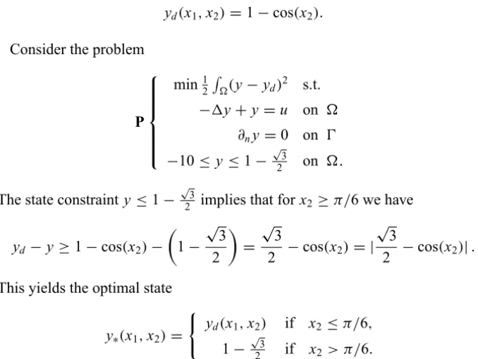
λ ω(λ) ey ev
10 π22 1.4758 0.1266 0 101/2 π22 1.4367 0.0883 0 1 π22 1.3705 0.0404 0 10−1/2 π22 1.3068 0.0165 0 10−1 π22 1.2711 0.0073 0 10−3/2 π22 1.2561 0.0010 0 10−2 π22 1.2509 3.6414e−04 0 10−5/2 π22 1.2493 2.3903e−04 0 10−3 π2
2 1.2487 2.0050e−04 0 10−7/2 π22 1.2486 2.2906e−04 0 10−4 π22 1.2485 1.5930e−04 0
Table 1 – Results as a function of the Lavrentiev-regularization parameterλwithu1=0 (non-prox Lavrentiev regularization).
The constraint violationevhas been computed as
ev=(0.001π )2
1000
X
i,j=0
(yc(xi j)−y∗(xi j))+ 2
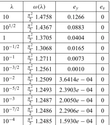
Starting withu1 = 0, we have computed the Lavrentiev-prox regularization iterates whithλk = 10∗10(1−k)/2. Letωk denote the optimal value ofP
λk,0,uk
which is used in the Lavrentiev prox iteration. Table 2 shows the results.
λk ωk ey ev
λ1=10 π 2
2 1.4758 0.1266 0
λ2=101/2 π 2
2 1.4188 0.0732 0
λ3=1 π
2
2 1.3323 0.0233 0
λ4=10−1/2 π 2
2 1.2694 0.0137 0
λ5=10−1 π 2
2 1.2514 0.0052 0
λ6=10−3/2 π 2
2 1.2486 0.0005 4.3289e−08
λ7=10−2 π 2
2 1.2484 1.8074e−04 1.6361e−07
λ8=10−5/2 π 2
2 1.2485 2.3783e−04 0
λ9=10−3 π 2
2 1.2485 1.5530e−04 0
λ10=10−7/2 π 2
2 1.2485 2.0268e−04 0
λ11=10−4 π 2
2 1.2485 1.3137e−04 1.0855e−11 Table 2 – Results for the Lavrentiev-prox iteration.
In this case the Lavrentiev-prox regularization iterates shown in Table 2 con-verge faster than the iterates generated with the non-prox Lavrentiev regulariza-tion shown in Table 1.
Figure 3 shows the optimal statey11that is computed in step 11 of the Lavren-tiev-prox iteration withλ11 =10−4.
Example 5. As in Example 4 let= [0, π] × [0, π]and define the desired stateyd(x1,x2)=1−cos(x2).
Consider the problem
P
min12R
(y−yd)
2 s.t.
−1y+y=u on
∂ny =0 on Ŵ
0.2pi 0.4pi
0.6pi 0.8pi
pi
0.2pi 0.4pi 0.6pi 0.8pi pi 0.02 0.04 0.06 0.08 0.1 0.12
x1 x2
y
Figure 3 – The computed statey11.
0
0.2pi 0.4pi
0.6pi 0.8pi
pi
0 0.2pi 0.4pi 0.6pi 0.8pi pi 0 0.5 1 1.5 2
x1 x2
y
The state constrainty ≤1 implies that forx2 ≥π/2 we have
yd−y ≥1−cos(x2)−1= −cos(x2)= |cos(x2)|. This yields the optimal state
y∗(x1,x2)=
(
yd(x1,x2) if x2≤π/2, 1 if x2> π/2.
Figure 4 shows the desired state yd and the optimal state y∗that is generated
by the optimal control
u∗(x1,x2)= (
1−2 cos(x2) if x2≤π/2, 1 if x2> π/2.
shown in Figure 5. The optimal controlu∗is continuous. The optimal valueω∗ ofPis given by the equation
ω∗= π 2
Z π
π/2
(yd−1)2 ds= π2
2
Z π
π/2
cos2(s)ds= π
2 2 0.25.
0.2pi 0.4pi
0.6pi 0.8pi
pi
0.2pi 0.4pi 0.6pi 0.8pi pi −1 −0.5 0 0.5
1 The optimal control
x1 x2
u
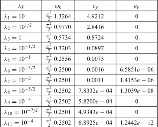
λ ω(λ) ey ev
10 π22 1.3264 4.9212 0 101/2 π22 1.0772 3.3972 0 1 π22 0.7380 1.6010 0 10−1/2 π22 0.4516 0.4012 0 10−1 π22 0.3175 0.0627 0 10−3/2 π22 0.2714 0.0089 0 10−2 π2
2 0.2568 0.0021 0 10−5/2 π22 0.2522 0.0010 0 10−3 π22 0.2508 7.3617e−04 0 10−7/2 π22 0.2504 7.0191e−04 0 10−4 π22 0.2503 7.6869e−04 0
Table 3 – Results as a function of the Lavrentiev-regularization parameterλwithu1=0 (non-prox Lavrentiev regularization).
As in Example 4, we use a discretization based upon Fourier-expansions. For v=P∞
j=0γjcos(j x2)the problemPλ,ε,vis equivalent to the problem
min
β∈l2 F(β) + ε 2
π
2
(β0−γ0)2+π
2 2
∞ X
j=1
(βj −γj)2
s.t. (19)
−10≤
∞ X
j=0
1 1+ j2 +λ
βj −λγj
cos(j x2)≤1, x2∈ [0, π].
By replacing the infinite series by a finite sum we obtain a semi-infinite op-timization problem with a quadratic objective function and linear constraints. Again in our numerical implementation we used the finite sums P75
j=0 and a finite number of inequality constraints corresponding to the 1001 grid points 0.001π j for j ∈ {0, . . . ,1000}. Again we used the program fmincon from the matlab optimization toolbox to solve the finite-dimensional optimization problems.
computed as in (17) and the constraint violationevhas been computed as in (18).
Starting withu1 = 0, we have computed the Lavrentiev-prox regularization iterates whithλk = 10∗10(1−k)/2. Letωk denote the optimal value ofP
λk,0,uk
which is used in the Lavrentiev prox iteration. Table 4 shows the results.
λk ωk ey ev
λ1=10 π 2
2 1.3264 4.9212 0
λ2=101/2 π 2
2 0.9770 2.8416 0
λ3=1 π
2
2 0.5734 0.8724 0
λ4=10−1/2 π 2
2 0.3203 0.0897 0
λ5=10−1 π 2
2 0.2556 0.0075 0
λ6=10−3/2 π 2
2 0.2500 0.0016 6.5851e−06
λ7=10−2 π 2
2 0.2501 0.0011 1.4153e−06
λ8=10−5/2 π 2
2 0.2502 7.8332e−04 1.3039e−08
λ9=10−3 π 2
2 0.2502 5.8200e−04 0
λ10=10−7/2 π 2
2 0.2501 4.9343e−04 0
λ11=10−4 π 2
2 0.2502 6.8925e−04 1.2442e−12 Table 4 – Results for the Lavrentiev-prox iteration.
Figure 6 shows the optimal statey11that is computed in step 11 of the Lavren-tiev-prox iteration withλ11 =10−4.
In this example the Lavrentiev-prox regularization iterates shown in Table 4 converge faster than the iterates generated with the non-prox Lavrentiev regular-ization shown in Table 3.
7 Conclusion
0.2pi 0.4pi
0.6pi 0.8pi
pi
0.2pi 0.4pi 0.6pi 0.8pi pi 0.2 0.4 0.6 0.8 1
The computed state
x1 x2
y
Figure 6 – The computed statey11.
that the Lavrentiev prox-iteration gives approximations of the same quality as the non-prox Lavrentiev regularization method in fewer steps and with larger regularization parameters. We have also applied the method successfully for the solution of optimal control problems with hyperbolic systems see [3].
Acknowledgements. The author wants to thank the anonymous referee for the helpful hints that have substantially improved this paper.
REFERENCES
[1] E. Casas,Control of an Elliptic Problem with Pointwise State Constraints. SIAM J. Control Optim.,24(1986), 1309–1318.
[2] E. Casas and M. Mateos,Second Order Optimality Conditions for Semilinear Elliptic Control Problems with Finitely Many State Constraints. SIAM J. Control Optim., 40(5) (2002), 1431–1454.
[3] M. Gugat and A. Keimer and G. Leugering,Optimal Distributed Control of the Wave Equation subject to State Constraints. To appear in ZAMM.
[4] A. Kaplan and R. Tichatschke,Stable Methods for ill–posed variational problems. Akademie Verlag, Berlin (1994).
[6] C. Meyer,Optimal control of semilinear elliptic equations with application to sublimation chrystal growth. Dissertation, Technische Universität Berlin (2006).
[7] C. Meyer and F. Tröltzsch,On an elliptic optimal control problem with pointwise mixed control-state constraints. Recent Advances in Optimization, A. Seeger, Ed., Springer-Verlag, (2006), 187–204.
[8] C. Meyer and A. Rösch and F. Tröltzsch,Optimal control of PDEs with regularized pointwise state constraints. Computational Optimization and Applications,33(2006), 209–228. [9] I. Neitzel and F. Tröltzsch,On Convergence of Regularization Methods for Nonlinear
Para-bolic Optimal Control Problems with Control and State Constraints, submitted.
[10] R.T. Rockafellar,Augmented Lagrange multiplier functions and applications of the proxi-mal point algorithm in convex programming. Math. Oper. Res.,1(1976), 97–116. [11] F. Tröltzsch and I. Yousept,A Regularization method for the numerical solution of elliptic
boundary control problems with pointwise state-constraints. Computational Optimization and Applications,42(2009), 43–66.
[12] F. Tröltzsch and I. Yousept,Source representation strategy for optimal boundary control problems with state constraints. Zeitschrift für Analysis und ihre Anwendungen,28(2009), 189–203.