Spatial analysis and investigation of fire events occurrences
in the Valencian Community, Spain
Spatial analysis and investigation of fire events occurrences in the
Valencian Community, Spain
Dissertation supervised by
Jorge Mateu, PhD
Department of Mathematics
Universitat Jaume I, Castellón, Spain
Co-supervised by
Pedro Cabral, PhD
Instituto Superior de Estatística e Gestão da Informação
Universidade Nova de Lisboa, Lisbon, Portugal
Edzer Pebesma, PhD
Institute for Geoinformatics
Westfälische Wilhelms-Universität, Münster, Germany
v
ACKNOWLEDGMENTS
I gratefully acknowledge the European Union Erasmus Mundus Scholarship program
for granting me and giving an opportunity to study Master in Geospatial
Technologies in the consortium universities. Except the acquired knowledge, my
thanks to this program are due to an unforgettable international and cultural
experience.
My sincere gratitude goes to my advisor Prof. Dr. Jorge Mateu for his technical
assistance and valuable comments during the thesis project and as well to my
co-advisors Prof. Dr. Pedro Cabral and Prof. Dr. Edzer Pebesma for the final
suggestions.
I want to thanks to all my colleagues for their friendship, professional advices and
assistance. It was pleasure to meat you.
I am also grateful to my parents who have supported me all the time. Special thanks
go to my sisters, Hugo, and friends in Croatia. Thank you for your moral support and
vi ABSTRACT
Fires have been affecting on average half a million hectares of forests, shrubland and
crops every year. During the second half of the 20th century with socio economic development people abandoned unproductive land and overpopulated more fertile
areas and cities. Landscapes started to be covered with natural vegetation or new
plantation, often with highly flammable flora (conifers, olive trees, fruit trees, etc.)
causing more frequent fire occurrences. Spain follows this trend with high incidence
of fires in recent years, underling and emphasising the importance of understanding
the causes and spatial distribution of these phenomena. In order to evaluate main
characteristics of fires and the distribution of ignitions, 3292 fire events detected in
Valencian Community during the period 2000 – 2006 are analyzed. GIS and spatial
point process modelling approach are used to quantitatively study the fire effects in
relation to variables such as cause, burnt area, proximity to urban areas and roads,
population density, land cover and geographic elements. Point pattern analysis was
performed using the library SPATSTAT with the statistical package R to determine
the spatial intensity of fire ignition distribution and how covariates affect the pattern.
Results showed that humans are the leading cause of fires in this region, but as well
that the Valencian Community has significant number of lightning caused fires. Fire
location are spatially clustered and high fire occurrences was found within areas
1 – 2 km from urban areas and roads, highly populated areas, in agricultural and
shrubland cover, lower elevations and tender slopes. Results suggested that there is
no simple fire regime for Valencian Community. The Akaike information criterion
method is used to select the best inhomogeneous Poisson process model from a set,
to best fit the data. The fitted model was diagnosed using simulation envelopes of K
function and residual analysis. The model turned out to be inadequate because the
fitted intensity function failed to capture the dependence of intensity on covariates.
Regardless that a satisfactory model was not found, the study emphasizes the
importance of understanding where fires occur and how they interact with
vii KEYWORDS
Fire occurrences
Geographic Information System
Inhomogeneous Poisson process
Intensity function
R
Spatial point pattern analysis
viii ACRONYMS
AIC Akaike Information Criterion
CLC CORINE Land Cover
CSR Complete Spatial Randomness
DEM Digital elevation model
EDF Empirical distribution function
EU European Union
GIS Geographic information system
HPP Homogeneous Poisson process
IGN Instituto Geográfico Nacional de España
SPP Spatial Point Pattern
UJI University Jaume I
ix
INDEX OF TEXT
ACKNOWLEDGMENTS ...v
ABSTRACT ... vi
KEYWORDS ... vii
ACRONYMS ... viii
INDEX OF TEXT ... ix
INDEX OF TABLES ... xi
INDEX OF FIGURES ... xii
1. Introduction ...1
1.1 Background information ...1
1.2 Fire ignition modelling ...2
1.3 Research objectives and hypothesis ...5
1.4 Study area ...6
2. Data preparation ...8
2.1 Analysis tools ...8
2.2 Data ...8
2.2.1 Fire ignition ...8
2.2.2 Land cover ...9
2.2.3 Anthropogenic variables ...11
2.2.4 Topographic variables ...13
3. Methods ...15
3.1 Analysis in GIS environment ...15
3.2 Spatial point pattern ...15
3.2.1 Test of complete spatial randomness ...16
3.2.2 First and second order properties ...16
3.2.2.1 Quadrat counting method ...18
3.2.2.2 Kernel smoothing ...18
3.2.2.3 Distance methods ...19
3.2.2.3.1 Empty space distances F ...19
x
3.2.2.3.3 Pairwise distances K ...20
3.3 Spatial point pattern modelling ...21
3.4 Model selection and evaluation ...22
4. Results ...24
4.1 General characteristics of fire events occurrences ...24
4.2 Fire ignition and covariates ...26
4.3 Test for Complete Spatial Randomness ...27
4.4 Model fitting and goodness of fit ...32
5. Discussion and recommendations ...36
6. Conclusion ...40
References: ...41
APPENDICES ...46
Appendix A: Anthropogenic variables (raster) ...46
Appendix B: Fire characteristics ...47
Appendix C: Visual results of interaction between fires and covariates ...49
Appendix D: Quadrat counting based on covariates and window (4x4) ...50
xi
INDEX OF TABLES
Table 1: Land cover classes based on CORINE nomenclature and area statistics ... 11
Table 2: Wildfire occurrence related to vegetation cover type ... 24
Table 3: Summary results of the quadrat counting method for testing CSR ... 29
xii
INDEX OF FIGURES
Figure 1: Study area, Valencian Community ... 7
Figure 2: Burnt area (left) and generated ignition hotspots (right) in Valencian Community . 9 Figure 3: Categorized CORINE Land cover 2000 in Valencian Community ... 10
Figure 4: Ignition hotspots superimposed over population density map (left), urban areas (center) and main roads (right) ... 12
Figure 5: Ignition hotspots superimposed over elevation map (left), slope map (center) and aspect map (right) ... 13
Figure 6: Distribution of fire ignition hotspots caused by human activities, either deliberate (a), negligence (b) or agricultural burning (c) and lightening caused fires (d) ... 25
Figure 7: Covariates used for modelling intensity function of fire events distribution... 27
Figure 8: Spatial intensity of fires and corresponding perspective surface for testing CSR .. 28
Figure 9: Spatial intensity of fires, temporal evolution for the years 2000 – 2006 ... 30
Figure 10: EDF plot of empty space and nearest neighbour distances (solid curve); upper and lower envelopes from 19 simulation of CSR ... 31
Figure 11: EDF plot of pairwise distances (solid curve); upper and lower envelopes from 19 simulation of CSR ... 31
Figure 12: EDF plot of inhomogeneous K function; upper and lower envelopes from 50 simulation of inhomogeneous Poisson process ... 33
Figure 13: Comparison of fire events in VC (left) and fire events predicted by fitted model (right) ... 34
Figure 14: Residual lurking plots of continuous covariate effects and diagnostic plot for spatial trend (four panel plot) ... 35
Figure 15: Calculated Euclidian distances (distance to urban area and main roads) and population density ... 46
Figure 16: Trend in burnt area and number of fires in the period from 2000 to 2006 ... 47
Figure 17: Distribution of the fire hotspots over the years ... 47
Figure 18: Proportion of land cover damaged in fires in period between 2000 and 2006 ... 47
Figure 19: Causes of the fires in Valencian Community ... 48
Figure 20: Occurrences of fires caused by human activities (left) and lightening (right) depicted in each land cover class ... 48
Figure 21: Fire characteristics in relation with land cover and topography covariates ... 49
1
1. Introduction
1.1 Background information
Fires are an integral part of many terrestrial ecosystems, including the Mediterranean
ones where they are a dominant ecological factor (Pausas 2001). They affect on
average half a million hectares of forest, shrublands and crops every year (Silva et al.
2010). In recent years there has been a significant high trend of number of fires and
burnt surface in European Mediterranean areas. One of the most affected regions is
Spain (European communities 2004).
There are several important characteristics that make the landscape of Mediterranean
Basin (MB) different from those of the rest of the Europe; climate (typically
characterized by summer droughts), the long and the intense human impact and the
role of fire influenced by the other two (Pausas and Vallejo 1999). Millennia of
severe pressure resulting in burning, cutting and grazing non arable land, clearing,
terracing and cultivating arable areas have created an area of strongly human
modified landscape (Pausas et al. 2008). With industrial development, European
Mediterranean countries have faced coastal urbanization, rural depopulation and
agricultural mechanization. The Valencian region in Spain succumbed to changes as
result of practices such as relocation of the people to the coastal border, farm and
grazing abandonment inland, a drift from traditional agriculture to industrial, leading
to intensification of agriculture, and tourism economics (Symeonakis et al. 2001,
Aguilar et al. 2006). Changes in traditional lifestyles caused progressive land
abandonment of large areas which led to the recovery of the vegetation (increase in
the cover and continuity of early succession species), but consequently fuel
accumulation as well (Houérou 1993, Pausas and Vallejo 1999). Amount and degree
of human alteration in the landscape pattern led to changes in the fires regime
(Moreira et al. 2001). Beside the human impact, an important factor of increased fire
2
fire risk and fire spread (Pausas and Vallejo 1999, Moreno 2010). As a result those
trends make European MB more fire prone.
1.2 Fire ignition modelling
Fires are not randomly distributed: vegetation, climate, topography and human
activities determine their spatial pattern (Gosalbo 2006). Fires introduces very
different dynamics over large areas with a tendency of differentially geographic
occurrences in space, being more frequently repeated in certain topographic location
or land cover types (Vázquez and Moreno 2001).
The majority of wildfires in Spain are caused by human activities (Pausas and
Vallejo 1999, Calcerrada et al. 2008, Moreno et al. 2010). Fires are an important
landscape disturbance which interacts in a complex way with land use land cover
changes. During the last three years all the areas burned in the larges EU
Mediterranean countries are areas close to or at intermediate distance to roads or
towns. Those area burns most frequently (Moreno 2010, Silva et al. 2010). Studies
have shown that those variables are significant in determining fire risk. For example,
(Calcerrada et al. 2008) found in his research, using the method from Bayesian
statistics, the weights of evidence (WofE) model, that spatial pattern of wildfires
ignition in south west part of Madrid region were strongly associated with human
access to the natural landscape, with proximity to urban areas and roads and one of
the most important causal factors. In recent years wildfires risk models that consider
other human variables such as distance to recreation areas, air pollution or population
density as explanatory variables have become common (Syphard et al. 2007, Tallut
and Suding 2008). Using index of topographic roughness and estimates of human
population density to model the frequency of fire with regression analysis (Guyette
and Dey 2000) verifies that at low population densities fire frequency increases as
population density does. Although it is assumed that land use change and human
activities in MB is the main reason of the increase in the number of fires and burnt
3
environmental factors (e.g. climate, soils, terrain topography) contributing to the risk
of fire ignitions that should be considered.
Several authors (Torn and Fried 1992, Hoffman et al. 2002) have addressed the
possible impact of global warming on wildfires using a global circulation model
(GCM). Over the years researchers have studied changes in climate and consequent
changes in fire hazards in Mediterranean ecosystems as well (Piñol et al. 1998,
Pausas 2001). They used correlation and regression analysis to validate the
significance of relationships giving confirming results. However, a lot of research is
focused on socio economic factors because there are more human caused fires than
natural ones. For example, registered lightning caused fires in Spain in the last 50
years were a very few, only 5% of the fires with known cause (Pausas and Vallejo
1999, Moreno 2010).
Many studies have found that topographic elements (elevation, slope and aspect) and
fuel characteristics (type, moisture and inflammability) are prominent factors on
shaping spatial pattern of natural caused fires (Kushla and Ripple 1997, Vasconcelos
et al. 2001, Rayan 2002, Yang et al. 2007). Those variables determine the fire regime
by controlling fire spread, intensity and extent (Guyette and Dey 2000). For example,
in the (Silva et al. 2010) research elevation positively influenced ignition
distribution. It is assumed that this effect may be due to some human activities
typical for higher elevation such as renovation of pastures for livestock using
traditional burning, which are also known as frequent cause of wildfires in the
Iberian Peninsula. On the other hand, (Vasilakos et al. 2009) found that elevations
have a small contribution to fire ignitions in Lesvos Island in Greece.
Numerous factors worldwide have been identified as factors influencing the spatial
pattern of fire ignitions distribution. However, we can see, the effects of different
factors on fire ignition occurrence can vary a lot among ecosystems and across
spatial scales (Yang et al. 2007). Findings are different indicating that fire itself is a
dynamic complex process that varies in time and space. Driving factors that affect
4
The investigation of ignition causes, ability to understand and predict the pattern of
ignition is crucial if we want to understand the important role and relationship
between fire regime, weather, vegetation, topography and human activities. It is
essential for fire management planning, policy decision and fire prevention. This
relationship can be investigated from many perspectives.
A fire modelling method consists of three fundamental components: fire occurrence,
fire spread and fire effects (Keane et al. 2004). Field investigation of the cumulative
effects would require excessive amount of time and money not available to many fire
scientist, thus models are helpful alternative tool used to understand and to predict
possible fire behaviour. Fire disturbances can be simulated spatially using either
mechanistic or stochastic strategies (Hong and Mladenoff 1999). Mechanistic
approach typically focus on a single fire event, while stochastic approaches often
focus on multiple fire events over long time periods. Therefore the replication of
individual fire events is not a goal of this research, rather the work focus on the large
scale characteristics of the historical fire occurrence. The stochastic strategy
simulates ignitions randomly or from probability functions of fire starts using
vegetation characteristics, climate indicators, topographical setting and/or other
parameters as independent variables (Keane et al. 2004). The entire complex ignition
process is often modelled using stochastic approaches where the probability of a fire
start is approximated from fire history (Johnson and Gutsell 1994, Boychuk et al.
1997), which will be implemented in this work.
Spatial statistical methods make it possible to determine whether or not fires are
more likely in some places than in others, and whether fires are more likely to be
found in a cluster or at some distance from one another (Podur et al. 2002). One of
the techniques is Spatial Point Pattern (SPP) which can be useful in modelling the
spatial pattern of fire ignition location as shown in different literature (Podur et al.
2002, Genton et al. 2006, Yang et al. 2007, Hering et al. 2009, Juan et al. 2010).
Recent theoretical development within the SPP techniques, such as formal likelihood
based methods of inference for a wide range of models, provides tools for
statistically rigorous modelling of spatial patterns of fire occurrence (Yang et al.
5
The paper presents an analysis of a spatial data set of historical fire occurrence
records in Valencian Community (VC) with the intent of quantifying a spatial model
of fire distribution intensity. It examines the significance of environmental and social
economic factors that may influence the presence and number of fires in VC. Fire
ignition is analyzed as a function of topographic elements; elevation, slope and
aspect, land use, depicted as well by spatial determinants such as distance to the
urban areas and distance to the main roads and population density. These factors will
be used as a potential explanation of the spatial variation of ignition density.
1.3 Research objectives and hypothesis
This work focuses on mapping and analysing fire ignition occurrence in VC over the
period between 2000 and 2006. The aim of this study was to use GIS techniques for
obtaining better understanding of conditions that relate to wildfires ignition
variability and the main causes of ignition. Likewise, parametric and non parametric
statistical analysis is used with an aim to describe and model spatial point pattern of
fire ignition density. Point pattern of fires will be tested against Complete Spatial
Randomness (CSR) to see whether data distributions exhibit random, clustering or
regularity. Seven independent explanatory variables are used (elevation, slope,
aspect, distance to urban areas, distance to roads, population density and land cover),
selected due to the possibility of their influence on wildfire ignition occurrence.
The specific objectives of this work are to assess:
1) The pattern and trend in the fire number and area burned, as well as the main
cause of fire activities
2) The influence of environmental and human variables on six year fire
activities
3) How the intensity of points fire events varies across the study area
In this research it is expected that, due to high human influence over the region and
because most of the fires are human caused, locations close to the roads and urban
6
population density is relatively low and there is a little variation over the region, it is
expected that the higher density of a fire ignition will be found in areas with a higher
population density. Land cover was also hypothesized to be an important determinant
of fire occurrence as vegetation in the Mediterranean climate region is dominated by
woody, evergreen and sclerophyllous shrubs that are very flammable (Syphard et al.
2009) and due to fact that human activities have dramatically increased fire
frequency as a consequence of land abandonment and tourist pressure (Pausas and
Vallejo 1999). It is hypothesized that topography elements helps to determine the
likelihood of fire occurrence as some configurations of the earth’s surface are more
prone to the fires. With respect to spatial fire distribution it is reasonable to assume
that fuel and heat are not homogeneous across landscape, thus it is expected to find a
non CSR spatial point process.
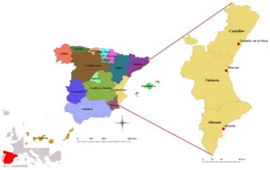
1.4 Study area
The Valencian Community is an autonomous community of Spain located in central
and south eastern part of Iberian Peninsula. It is situated at 39° 28 N latitude and 0°
22 W longitude geographic coordinates (Figure 1). It covers an approximate area of
23273.439 km2. Administratively, the VC is divided into three provinces: Alicante, Valencia and Castellón.
The VC today has a population of about 5.1 million people, which represents 10.9%
of Spain. The average population density is 219.3 inhabitants per km2, but with highlighted demographic imbalance, with the majority of the population concentrated
on the coastal strip. 53% of the Valencian population lives in the coastal towns
(Cámara Valencia 2010). The variation in population density is derived from a
traditional concentration of people in localities with fertile cultivation and growing lowlands by the most important rivers (Júcar, Turia, Segura, Vinalopó), as well as harbour cities important for the agricultural trade. In VC land use/land cover change
caused by urban growth has affected especially the metropolitan cities of the coastal
plains. In these areas the soil is highly productive and can support an intensive and
7
climate, heavily influenced by the neighbouring Mediterranean Sea. Proper
Mediterranean climate is typical along the coastal plain (518 km), characterized by
warm and dry summers and mild winters, changing to continental climate inland. Hot
summers and around 100 days of sun per year has influenced on development of a
significant beach tourism infrastructure and inland depopulation (Cámara Valencia
2010).
Figure 1: Study area, Valencian Community
Due to its climate, land use history and human activities one of the most fire affected
areas in Spain is the Valencian region (Delitti et al. 2004). Extensive grazing is being
progressively abandoned as a result of a desertion of the country side to urban
centres. Due to lower demand of fuel wood and charcoal there is increasing buildup
of fuel in forest and shrub land. Furthermore, the VC is third tourist destination in
Spain (Cámara Valencia 2010). All together, fuel buildup and intense tourist traffic
8
2. Data preparation
2.1 Analysis tools
Mapping, editing tasks and map based GIS analysis were made using ArcGIS
Desktop version 9.3. The main tool for statistical analysis is the open source R
environment for statistical computing, version 2.12.0 (The R Project for Statistical
Computing). Microsoft Office Excel 2007 was used for computing and tabulation of
data. All the data are in shape file format, represented in a projected Coordinate
System ETRS89 with Universal Transverse Mercator (zone 30) projection.
2.2 Data
In this study emphasis was directed on territory characteristics related with human
presence and activity. In order to analyze spatial distribution and characteristics of
fire ignition the following digital cartography were prepared.
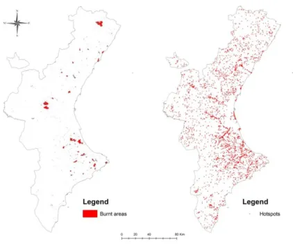
2.2.1 Fire ignition
Fire data of VC used for this project are property of Conselleria de Medi Anbient,
Generalitat Valenciana which are granted to University Jaume I (UJI) for research
purposes. The fire data consist from polygons of burnt areas for the period of six
years, from 2000 to 2006. The data contain additional fire characteristics such as
cause of the fires and the date of fire occurring. It is considered that the area is burnt
only once, thus if there was overlapping between polygons of burnt area preference
is given to the more recent fire. From the initial 3309 polygons of burnt area, after
9
calculated. To represent an estimated hotspot of a fire ignition, centroids were
generated. Figure 2 depicts a map of burnt areas and generated hotspots.
Figure 2: Burnt area (left) and generated ignition hotspots (right) in Valencian Community (period 2000 – 2006)
2.2.2 Land cover
CORINE Land Cover (CLC) cartography inventory for the year 2000 in scale
1:100 000 and with the surface area of the smallest mapping unit of 25 ha was obtained from the Instituto Geográfico Nacional de España (IGN). CLC is a map of the European environmental landscape based on interpretation of satellite images. It
provides comparable digital maps of land cover for each country for much of Europe.
Land cover classes used for this research are defined based on a CORINE
nomenclature (CLC classes). Initially, 44 land cover classes where categorized into
10
agriculture, 4) forest, 5) shrub and herbaceous vegetation and 6) wetland and water
bodies (Figure 3). The description of class’s inclusion and areas statistics are
exhibited in Table 1.
Figure 3: Categorized CORINE Land cover 2000 in Valencian Community
Land cover pattern within the study area have obvious spatial distribution
characteristics from sea to inland. Most of the infrastructure and economic activities
of the region are concentrated in a coastal zone. Near urban areas, going toward
inland, dominates agriculture, mostly cultivable land, extended on 22% of VC land
and heterogeneous agriculture around 23.51%. Most represented land cover types of
this region is shrub and/or herbaceous vegetation (35.66%). Forest make up only
11
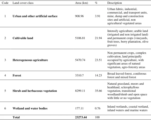
Table 1: Land cover classes based on CORINE nomenclature and area statistics
Code Land cover class Area (km) % Description 1 Urban and other artificial surface 908.96 3.91
Urban fabric, industrial, commercial, and transport units, mine, dump and construction sites and artificial, non agricultural vegetated areas
2 Cultivable land 5106.81 21.94
Intensify agriculture; arable land (irrigated and non irrigated land) and permanent crops (vineyards, fruit trees, berry plantation, olive groves)
3 Heterogeneous agriculture 5470.74 23.51
Non permanent crops, complex cultivation, land principally occupied by agriculture, with significant areas of natural vegetation, agro-forestry areas 4 Forest 3310.7 14.23 Broad leaved forest, coniferous forest and mixed forest
5 Shrub and herbaceous vegetation 8299.11 35.66
Natural grassland, moors and heathland, sclerophyllous vegetation, transitional woodland/shrub and open space with little or no vegetation 6 Wetland and water bodies 177.11 0.76 Inland wetlands, coastal wetland,
inland waters and marine waters
Total 23273.44 100
2.2.3 Anthropogenic variables
These maps were produced using BCN 200 (Cartographic Numeric Database of
Spain Base in scale 1:200 000) for VC obtained from IGN. Specifically, vector shape files of municipalities, municipality’s capitals and other settled areas, and roads (motorways, national and autonomous roads). All vector data were overlayed with
12
Figure 4: Ignition hotspots superimposed over population density map (left), urban areas (center) and main roads (right)
Population density (number of persons per km2) was calculated from 2008 census data, the number of persons present in each municipality, using attribute information
which was contained in the municipality shape file. These values were divided with
corresponding areas. This component of human population density does not reflect
changes in population density over time, rather it is static variable and it is assumed
no or very little changes in population density over observed period and census data.
In 75% of the territory live not more than 2 persons/km2, however this correspond to just 7% of the VC population.
Using vector shape files (cities and roads) and calculated Euclidian distance, a raster
was generated representing distances to urban areas and respectively distance to main
roads. From the center of the source cells (urban areas or roads) it was calculated all
the distances to the center of each of the surrounding cells. This raster data will be
13
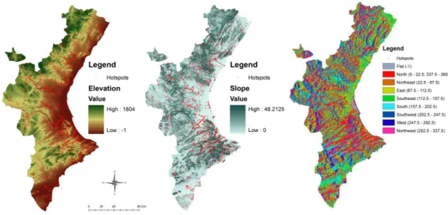
2.2.4 Topographic variables
Determining the relationship between topographic features of the terrain and fire
occurrences is important for evaluating the activities of fire (e.g. the rate and
direction of fire spread). In order to analyze fires as a function of topographic
attributes a digital elevation model (DEM) of the study area is used. DEM in ASCII
format with 200 m spatial resolution was obtain from IGN and converted to raster.
Topography is usually broken into following categories which were derived from
DEM: elevation, slope and aspect (Figure 5). Elevation and slope are represented as
continuous variables, while aspect was reclassified and introduced as factor in nine
categories; flat (F), north (N), northeast (NE), east (E), southeast (SE), south (S),
southwest (SW), west (W) and northwest (NW).
14
From DEM it was observed main characteristics of the study region. The average
height of VC is 869.56 m, with minimum of -1 m, maximum of 1804 m of land
height and 504.07 m of standard deviation. The slope of terrain varies from 0 to
48.21 degree, but around 79% of the territory have slope less than 10 degree (mean
value is 6.15 degree and standard deviation of 5.75 degree). In the terms of the
15
3. Methods
This section describes GIS and statistical methods employed to achieve desired
objectives in order to explain fire ignition occurrence in VC based on a set of
explanatory variables. The entire R code used in the statistical part of the study is
presented in Appendix E.
3.1 Analysis in GIS environment
Fires were analyzed a priori purely descriptively to obtain a general view and idea
regarding spatial-temporal fire characteristics itself and in context with other
variables. All thematic maps were further treated and incorporated into the same GIS
environment to create different cartographic overlays and subsequent analysis of a
fire regime to make inferences about historical fire activities, and consequently about
future ones as well. Based on the data, the relation between fires and landscape,
population density and socio economic variability were quantified. Combination of
different thematic layers have been undertaken in order to determine the trend of
fires, spatiotemporal dynamics observed in the terms of burnt area, number of fires
and seasonality and the most frequent burned vegetation types, human activities and
terrain characteristics assuming the pre fire conditions.
3.2 Spatial point pattern
SPP is a set of events irregularly distributed within some region and presumed to
have been generated by some form of stochastic mechanism (Diggle 2003). These
points might represent trees, animal’s nests, cases of disease, fire location or location
of any other naturally occurring phenomena. SPP analysis usually starts with
16
probability distribution over observed region. In point patterns any kind of additional
data at every spatial location may be used as explanatory variables (covariates) for
point distribution. For the point pattern covariate analysis the study adopted methods
proposed by (Baddeley 2008) implemented in R statistical package SPATSTAT
(Baddeley and Turner 2005).
3.2.1 Test of complete spatial randomness
The test of complete spatial randomness (CSR) is usually considered as the
appropriate starting model for a point pattern (Mateu 2004, Baddeley 2008). A
collection of events is considered to be completely spatially random (uniformly
distributed over space) if the intensity λ is constant over space and events are neither
clustered nor regularly spaced (Podur et al. 2002). A point process which is CSR
point process is formally defined as homogeneous Poisson process (HPP). The first
basic task in analysing a point pattern is rejection of CSR as it is a minimal
prerequisite for any serious attempt to model an observed pattern, as CSR operates as
a dividing hypothesis between regular and aggregated patterns (Mateu 2004). First
and second order properties are often used for characterization of a point pattern and
testing if there is evidence against CSR. Each the property is the focus of different
analysis.
3.2.2 First and second order properties
First order properties measure the distribution of events across study area while
second order properties describe the covariance between values of the process at
different regions in space measuring the tendency of events to appear clustered,
independently or regularly spaced (Gatrell et al. 1996).
First order properties are described in terms of the spatial intensity λ(s) defining the
17
following in (Equation
1)
, where ds is a small region around the point x and Y(ds) refers to the number of events in this small region.
(Equation 1)
The second order properties, or spatial dependence of a spatial point process involve
the relationship between numbers of events in pairs of sub regions within R (Gatrell
et al. 1996). It is a measure of how close events are to each other, indicating
clustering or regularity. If the point pattern reflects clustering, points will tend to be
closer to each other than expected for a Poisson process. Respectively, for regularity
points will tend to avoid each other and be farther apart from one another than a
random distribution would suggest (Podur et al. 2002). The second order intensity
function is defines in (Equation
2)
.
(Equation 2)
Intensity may be uniform or homogeneous or may vary from location to location
(inhomogeneous). If the point process is homogenous, then for any sub region
expected number of points is proportional to the area. Hence, the constant intensity λ
is expected. However, it is more likely that intensity will vary across area influenced
by different factors (Diggle 2003, Baddeley 2008). Until first order intensity is taking
into account only the location of events, the second order intensity function depends
on the distance between events, not the exact location.
An exploratory tool for examining the first order properties and a classical test for
the null hypothesis of CSR is the χ2 (chi – squared) test based on quadrat counts and Kernel smoothing. As well, several functions based on distance may be used to
18
3.2.2.1 Quadrat counting method
With this approach the study region is divided into sub regions or quadrats of equal
area and the number of events in each quadrat are counted. Under the null hypothesis
of CSR the number of points in each sub region is independent and identically
distributed (equal number of events per region - expected). From a theoretical
viewpoint, the quadrats do not have to be of equal area and could be regions of any
shape, but the counted number of points for HPP should be proportional to the
region. Any choice of quadrats is permissible. It is more useful if we choose the
quadrats in a meaningful way. We can define quadrats using covariate information to
test whether the point pattern intensity depend on a covariate (Baddeley 2008), which
was implemented in this work as well.
The Pearson χ2 goodness of fit test is a formal test of the null hypothesis that the model is true against a very general alternative that the model is not true. The test is
using Pearson residuals validation (Equation 3). If the data is Poisson it will aspire to
zero.
(Equation 3)
3.2.2.2 Kernel smoothing
While the quadrat method gives a global idea of sub regions and related intensity,
Kernel technique produces a more spatially “smooth” estimate of the variation of the
probability density (Baddeley 2008).
This technique uses a moving three dimensional function (the kernel) which weights
events within its sphere of influence according to their distance from the point at
19
points that are further away less than those that are close. The usual kernel estimator
of the intensity function is defined in (Equation
4)
, where k(u) is the kernel and e(u) edge effect correction.
(Equation 4)
.
Kernel density algorithm is implemented in SPATSTAT giving as a result a raster
display representing the resulting intensity estimates as a continuous surface. This
show how intensity varies over the observed region.
3.2.2.3 Distance methods
The classical techniques for investigating inter-point interaction are distance
methods, based on measuring the distances between points. The general approach of
methods is to calculate empirical distribution function (EDF) of a point pattern and
compare it against theoretical distribution function under CSR. Typically analysis is
performed using simulation envelopes. By calculating n number of independent EDF
simulation under CSR it is defined upper and lower simulation envelopes, which is
plotted against EDF. EDF outside of upper and lower envelopes indicate rejection of
CSR (Diggle 2003).
3.2.2.3.1 Empty space distances F
The empty space function F (point to nearest event) of a point process is the
cumulative distribution function of the distance ei from a fixed point in space to the
nearest point of each m sample of a point pattern. Inference is typically conducted by
20
Values F(t) > Fpois(t) suggest that empty space distances in the point pattern are
shorter than for a Poisson process, indicating regularity, while F(t) < Fpois(t) suggest
a clustered pattern. The Fpois(t) and EDF of empty space distance F(t) are defined in
(Equation
5)
, where # means “the number of” (Diggle 2003, Mateu 2004).
(Equation 5)
3.2.2.3.2 Nearest neighbour distances G
The nearest neighbour distance distribution function G (event to event) of a point
process is the cumulative distribution function of the distance di from a random point
to the nearest other point of a point pattern. Interpretation of G(t) is the reverse of
F(t). Values G(t) > Gpois(t) suggest that nearest neighbour distances in the point
pattern are shorter than for a Poisson process, indicating clustering, while
G(t) < Gpois(t) suggest a regular pattern. G(t) and Gpois(t) are given in (Equation 6).
(Equation 6)
3.2.2.3.3 Pairwise distances K
Pairwise distances (variously known as the reduced second order moment function or
Ripley's K function) is a stationary point process so that λK(t) is the expected number
of other points of the process within a distance t of a typical point of the process. K
statistic use the distances between all neighbours in a point pattern and it is a
21
(Equation 7)
Values K(t) > Kpois(t) suggest clustering, while K(t) < Kpois(t) suggest a regular
pattern.
3.3 Spatial point pattern modelling
The point process models fitted to the data are often specified in terms of its
conditional intensity (Papangelou). Conditional intensity interpret probability of
having an event at point u given that the rest of the point process coincides with x
(Baddeley and Turner 2000). In practice, the conditional intensity is normally
specified through a loglinear form (Equation 8) where θ1 and θ2 represent parameter
to be estimated.
(Equation 8)
The trend term B(u) depends only on the spatial location u, so it represents spatial
trend or spatial covariate effects. The interaction term C(u, x) depends beside on the
point u and on the configuration of x. It represents stochastic interactions between
the points. The term C(u, x) is reduced to zero for the Poisson process (Baddeley and
Turner 2000). R software currently fits models by the method of maximum
22
3.4 Model selection and evaluation
The effective way to choose between a set of models is to use Akaike Information
Criterion (AIC). The AIC is a measure of goodness of fit that takes the number of
fitted parameters into account (Dalgaard 2008). “True model” does not have to be in
the set, the goal is to select the best approximating model of set (Burnham 2004). It
is widely used as a measure for selecting the best among competing models for a
fixed data set (Yang et al. 2007). AIC is described as in (Equation 9), where k is the
number of parameters and L is the maximized value of the likelihood function for the
estimated model. The smaller AIC values favours a better fit of the model to the
observed data.
(Equation 9)
Although summary statistic such as K function are intended primarily for exploratory
purposes, it is possible to use them as a basic for statistical inference (Baddeley
2008). Thus, simulation envelopes of K function were used for testing realization of
a finally fitted model, but instead of assumption that the null hypothesis was CSR,
the simulated process was generated according to the fitted model, taking into
account ihnomogeneity. The inhomogeneous K function supposes non constant
intensity at each location of a point pattern, so each point xi will be weighted by
ωi=1/λ(xi). The inhomogeneous K function is given in (Equation
10
below (Mateu2004):
23
As well, residual diagnostic plots, recently formulated by (Baddeley et al. 2005) that
plot residual against a spatial continuous covariates, was used as a additional
24
4. Results
4.1 General characteristics of fire events occurrences
According to the results obtained by the analysis of cumulative fire incidences during
the 6 year period around 1% of the VC region has been burned (25323.20 ha). From
2000 to 2006 average burnt surface every year was 7.69 ha with standard deviation
of 99 ha. Province Valencia is the most affected with 11717.26 ha of burnt area,
followed by Castellon with 7698.80 ha and Alicante with 5907.14 ha. Fires mostly
affected shrub and herbaceous vegetation (70.06%) and 14.47% of influenced area
were forests (Table 2).
Table 2: Wildfire occurrence related to vegetation cover type
Code Land cover Burnt area (ha)
% of total burnt area 1 Urban and other artificial
surface 129.82 0.51
2 Cultivable land 1395.39 5.51
3 Heterogeneous agriculture 1781.85 7.04
4 Forest 3663.85 14.47
5 Shrub and herbaceous
vegetation 17740.4 70.06
6 Wetland and water bodies 611.89 2.42
Total 25323.2 100
From a total of 3292 fires, small fires (< 1ha) make 70% of fires, however the burnt
area of these fires is less than 1% (220.71 ha). The rest of the burnt territory was
burnt by fires bigger or equal than 1ha (25102.49 ha). Almost 60% of the burnt area
is caused with wildfires bigger than 500ha.
More than 50% of the fires were caused due to human reasons, either deliberate or
25
fires. Agricultural burning, bonfire, smoking, forestry work, grass burning and fires
caused by engines and motors rise percentage on human direct and indirect caused
fires on more than 65%. Natural fires caused by lightening (ray) make 24% of total
fires. Distribution of those natural and non natural caused fires is very different as
well. Natural ones are mostly concentrated inland while fires caused by human
activities are aggregated in coastline region (Figure 6). Fires were also observed
separately through years. It is observed that the amount of burnt area has been
decreasing while the trend of number of fires was increasing.
The trend in burnt area and number of fires in each year, as well as cumulative
affected areas, different causes of the fires ignition in Valencian region and
frequency analysis to investigate where most common fires were ignited are
visualised in Appendix B.
26
4.2 Fire ignition and covariates
To analyse in which land cover fire mostly occurred, ignition hotspots were
superimposed on the CLC. Analysis showed that the fires in almost 60% of the cases
started in agricultural land, either cultivable land or heterogeneous agriculture.
31.75% fires started in shrub and herbaceous vegetation. Fires caused by lightening
in almost 50% of the cases happened in land cover of shrub and herbaceous
vegetation.
It has been explored quantitatively how distance to urban areas, main roads and
population density influence fire ignition occurrence. About 39% of fires occurred at
less than 500 m from main roads and 84% were within a distance of 2 km. Fire
hotspots were also located very close to the urban areas, with 6% at less than 500m
distance, and 53% of hotspots at less than 2 km. Most of the fires (72%) that
occurred were in areas of lower population density (less than 2 persons per km2). For map visualization refer to Figure 4.
Furthermore, in relation with topographic characteristics it is observed fire frequency
depending on elevation, slope and aspect. Results show decreasing trend of fire
frequency with increase of the terrain height. Around 38% of the fires were in
landscape lower than 200 m, 57% in areas higher than 200 m, but less than 1000 m
and only 4.6% of the fires were in elevations higher than 1000 m. As well, it was
observed decreasing trend of fire frequency with increase of the slope degree.
Around 79% of the fires happened in the terrain where slope is less than 10 degree,
17.65% where slope is between 10 and 20 degree and only 3% of the fires were in
the area with slope higher than 20 degree. By analyzing aspect characteristic and fire
occurrence frequency results show that the highest number of fires (more than 40%)
were detected in areas most suitable for fires; south (14.70%), southwest (9.75%) and
southeast (15.70%). High number of fires (13.91%) was detected as well in the slope
facing east. Interaction between fire ignition hotspots with topographic
27
In order to model the dependence of a point pattern on a spatial covariates following
in next part, all covariates were prepared in raster format and inserted in R
environment. Ignition point and the Valencian region were used as well (Figure 7).
Figure 7: Covariates used for modelling intensity function of fire events distribution
4.3 Test for Complete Spatial Randomness
Fire events in VC for period from 2000 till 2006 have been tested against CSR to see
whether data distribution exhibit random, clustering on regularity.
Under the null model of CSR, fire data has a constant intensity of 1.411480e-07
points per square meter over the region of VC. However, in general the intensity of a
point process will vary from place to place, thus it is suspected that the intensity may
be inhomogeneous. Applied methods of quadrat counts and Kernel smoothing for
testing this assumptions, gives a clear conclusion of fire events inhomogeneity.
In quadrat counting the window was divided into 4x4 sub regions, but as well
covariates information were implemented for dividing region in a meaningful way.
28
counts and the Pearson residual. If the point process is homogenous, then for any sub
region the expected number of points is proportional to the area, which is not the
case; the number of points in the sub regions is very different from expected. The
other indicator that fire dataset is inhomogeneous is P – value smaller than 0.05 in all
of the cases. For clear interpretation all numerical data are shown in the table below
(Table 3), while visualization of defined quadrats is presented in Appendix D.
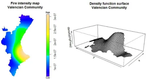
Using Kernel smoothing method it was created fire intensity raster map which
indicate concentration of points just in some areas, thus data indicate inhomogeneous
pattern From this two visualizing techniques (Figure 8) we can perceive the most risk
area is located in a coastal zone (colored yellow hues). Maps of the intensity for all
the years (2000 – 2006) are shown in Figure 9. These show the persistent in
distribution of hotspots with some minor deviations and in the most risk area.
29
Table 3: Summary results of the quadrat counting method for testing CSR
Elevation p-value < 2.2e-16 λ2=371.6536
1 2 3 4
O 1195 954 649 478 E 817.67 821.93 818.61 817.77
R 13.19 4.60 -5.92 -11.88
Slope p-value = 0.02298 λ2=9.5337
1 2 3 4
O 744 798 889 820 E 793.19 819.23 819.28 819.28
R -1.74 -0.74 2.43 0.02
Aspect p-value = 2.218e-06 λ2=40.8562
F N NE E SE S SW W NW
O 32 432 432 456 516 484 319 286 326 E 26.23 354.73 405.92 495.23 604.70 488.99 340.19 266.50 300.47
R 1.12 4.10 1.29 -1.76 -3.60 -0.22 -1.14 1.19 1.47
Population density p-value < 2.2e-16 λ2=227.4573
1 2 3 4
O 594 633 958 1097 E 822.77 823.33 819.48 816.41
R -7.97 -6.63 4.83 9.82
Distance to urban area p-value < 2.2e-16 λ2=362.8808
1 2 3 4
O 1233 885 646 510 E 819.25 826.50 808.14 820.09
R 14.45 2.03 -5.70 -10.82
Distance to roads p-value < 2.2e-16 λ2=229.2226
1 2 3 4
O 862 900 658 493 E 634.68 758.54 723.51 796.25
R 9.02 5.13 -2.43 -10.74
Land cover p-value < 2.2e-16 λ2=161.4492
1 2 3 4 5 6
O 138 783 800 414 1065 84 E 128.10 720.14 771.06 467.27 1172.31 25.09
R 0.87 2.34 1.04 -2.46 -3.13 11.75
4x4 quadrats p-value < 2.2e-16 λ2=688.6553
O 13 41 326 95 227 491 327 100 520 778 31 5 276 55 E 21.64 41.55 454.47 143.69 345.39 499.48 233.72 112.53 516.79 355.78 19.91 15.58 399.06 49.34 R -1.85 -0.08 -6.02 -4.06 -6.37 -0.37 6.10 -1.18 0.14 22.38 2.48 -2.68 -6.16 0.80
30
Figure 9: Spatial intensity of fires, temporal evolution for the years 2000 – 2006
Like mentioned in methodology part, a good way for inferring if the point pattern is
completely random or there is some spatial pattern is using the distance statistic. The
comparability of a point process with CSR is assessed by plotting EDF against the
theoretical expectation assuming CSR. For simulation 19 independent EDF under
CSR were chosen (Figure 10). In both cases, empty space and nearest neighbour
distances, EDF lies outside of simulated envelopes indicating rejection of CSR.
Further, plotted EDF of nearest neighbour distances is larger than all 19 simulations,
showing excess of small nearest neighbour distances which is a characteristic feature
of clustered pattern. Similarly, EDF of empty space distances below the lower
simulation envelope typifies cluster pattern as well.
Effective diagnosis of independence or dependence between points includes the K
function as well (Figure 11). How EDF is outside of simulated envelopes and
pairwise distances are smaller than expected under CSR, pairwise distance statistic
31
Figure 10: EDF plot of empty space and nearest neighbour distances (solid curve); upper and lower envelopes from 19 simulation of CSR
32
4.4 Model fitting and goodness of fit
Because the fire events did not fit into the null hypothesis that the distribution is
homogeneous Poisson the possibility of an inhomogeneous Poisson process was
explored with an intensity function that could be explained with spatial covariates
that were revealed to affect fire occurrence pattern; elevation, slope, aspect,
population density, distance to urban areas, distance to roads and land cover. All
possibilities, taking into account all possible combinations of covariates, accurately
127 models, was fitted to date. The final model was chosen based on the lowest AIC
value (AIC=107715.0). The best model among those investigated, was a function of
all seven covariates. Coefficients for intensity function are given in Table 4.
Variables with positive coefficients have positive contribution to the fire occurrence
density and negative coefficients have negative contributions.
Table 4: Coefficients of the predictor variable of the final fitted model
Fire ignition occurrences intensity function
Trend formula exp(~el + sl + factor(as) + du + dr + pd + factor(lc))
Intercept
- 15.82745
Elevation
- 0.001013557
Slope
+ 0.02421431
Aspect
+ 0.4816883 (N) + 0.4354635 (NE) + 0.3198927 (E) + 0.2056588 (SE) + 0.3498161 (S) + 0.3600464 (SW) + 0.5581428 (W) + 0.5039866 (NW)
Distance to urban areas
- 0.00013887
Distance to roads
- 0.00008669166
Population density
-0.00027228
Land cover
+ 0.3374982 (2) + 0.3604987 (3) + 0.5843269 (4) + 0.4698501 (5) + 1.397223 (6)
33
In order to test if suggested model for the intensity is a good representation of the fire
events that occurred in VC, 50 envelope simulations of the inhomogeneous K
function were generated according to fitted model (Figure 12). By using the
inhomogeneous K function the assumption of an underlying homogenous point
process is removed while still assuming isotropic stationarity (Hering et al. 2009).
The plot suggests that after accounting for dependence on covariates, the fitted model
is not the best possible interpretation since observed function in some parts lies
outside of the simulated envelopes. Model failed to capture dependence of intensity
and covariates for distances between 2.5 and 9 km and bigger than 35 km.
Comparison of simulated model and real fire distribution is shown in Figure 13,
giving a clear indication of an inadequate model.
34
Figure 13: Comparison of fire events in VC (left) and fire events predicted by fitted model (right)
Diagnostic plots and residuals are a useful tool for a quick indication of departure
from the trend in the model and the covariate effect (Baddeley et al. 2005). Residuals
are plotted against the covariates and Cartesian coordinates to assess how the true
spatial trend differs from one specified by the fitted model. For the spatial covariate
defined at each location evaluated residual should be approximately zero if the fitted
model is correct. Diagnostic plots (Figure 14) suggest that the fitted model
underestimated the intensity regarding to all continuous covariates. Take the
elevation as an example (Figure 14a). The cumulative Pearson residuals are much
less than +2σ limit of error bounds for elevations between 100 - 200 m and 600 - 750
m, suggesting that the model overestimate intensity of fire occurrences at this scale.
There are less fires occurring at those spatial locations than fitted model predict.
Residuals much higher for elevations around 200 – 250 m and bigger than 14 km
suggests that there are more fires at this scale. The steepest increase is between 100 -
200 m and 700 m – 1 km indicating that highest number of fires is ignited at those
elevations. Respectively, the peak in Figure 14b occurs for slopes of about 2.5 degree
and the steepest increase occurs within range of slopes of 2.5 – 8 degree, suggesting
that more fires occur on gentle slopes than steeper ones. There is less fire at mild
slopes (< 10 degree) and more fires at steeper at spatial location then fitted model
35
areas with higher population density. The peak is at about 2 indicating that most fires
occur within an area of low population density. The fitted model has deficit of fire
events for the distances lower than 3 km and excess for distances approximately
between 4 and 8 km from the urban areas. In other words, there are more fires
occurring at spatial locations near to roads then fitted model predict (Figure 14d).
There is a steep increase of cumulative residuals after the nadir point (1 km)
suggesting that most of the fires were ignited at this scale. The lurking plot for
distances to the roads (Figure 14d) has similar behaviour as the plot for distances to
urban areas indicating that most fire ignition at distances 1 – 2 km from roads.
36
5. Discussion and recommendations
Fire events observed in VC confirm statistics of the Center for Fire Research
(Moreno 2010) that despite the increase in fire prevention and suppression effort, as
well as a decreasing trend in burnt area, during the last decades the number of fires
have continued rising. Probably the reason why fires started to be more frequent is
because of rural exodus and changes in life style which little by little accumulated
the vegetation fuel (Pausas and Ramos 2004). Particular caution should be directed to
forest fires as a second most affected cover in VC. The dynamics of recovery of
abandoned agricultural land toward forest, employing new technologies which use
great amount of fossil energy made the newly established ecosystem probably
generally fire prone (Ales et al. 1992). The facts that certainly does not help are also
new trends of more people living in urban forest interface and recreational activities
increased in forested areas (Calcerrada et al. 2008, Silva et al. 2010). As fires tend to
transform during the initial stages forest to shrubland and shrubland invasion is a
much quicker than that of forest, threat of increased fire frequency in those areas is
present. It is confirmed that herbaceous vegetation in many Mediterranean
agricultural areas is easier to ignite and the fires propagate more easily than in other
fuel types.
Comparing density of fire events obtained from quadrat with Kernel density
technique both show more dense concentration of fires in the area that follow coast
of VC and gradually decreasing going away from the central coastal region toward
the heartland. From the summary table of the quadrat method, as well supported by
GIS analysis, we can observe how covariates interact with fire distribution.
Distribution of fire data in VC is not random. There is obvious inhomogeneous
pattern with a strong preference of fires for lower elevations, mild slope facing high
potential solar isolation, higher population density, proximity to urban areas and
roads, agricultural land and shrub or herbaceous vegetation. The K(t) function, and
the two nearest neighbour distribution function, (F(t) and G(t), provided
complementary tools for the description of SPP indicating clustering of fire events.
37
CSR and for testing fitted model. EDF under the CSR showed clear results using 19
envelopes, which was not the case with simulations of the inhomogeneous K
function according to fitted model, thus it was used 50 simulations. The reason was
also long computation time.
Although the proposed model is inadequate because the fitted intensity function
failed to capture the dependence of intensity on covariates, all variables included in
this research should be incorporated in a trend. Lurking variable plots are helpful to
indicate whether or not the presence of a particular variable is needed in the model
(Hering et al. 2009). If cumulative residual function of the residuals against variable
of interest lies outside of the envelope, this is evidence that the variable should be
included in the trend for fitting the model. All covariates in earlier presented lurking
plots are partly outside of the envelopes.
How a minimum 50% of the fires in VC were caused by humans, all these types of
fires should be clustered around areas where people live, work and recreate, which is
confirmed in the Figure 6. Because humans caused the majority of fires, the measure
of accessibility represented as a distance to urban areas and roads is an important
explanatory factor reflecting the effect of human activities. It was found that the SPP
of ignition is associated with landscape accessibility in this area. Distances around
1-2 km of urban areas and roads are the peak of ignition findings and generally
associated with higher fire occurrences probabilities. Studies have already showed
that these factors are significant in determining fire risk, but as well contrary to what
may be believed, areas at intermediate distance to towns or roads might burn in
higher proportion than those closer (Moreno 2010).
Land cover, in terms of presence and impact of humans, showed a strong influence
on the probability of fire ignition, similar to other author’s findings (Lloret et al.
2002, Silva et al. 2010). Significant number of fires occurred in agricultural areas
indicating importance of this factor on influence of fire starts. As VC has strong
agricultural community, land management such as burning agriculture residues, land
burning for pasture renovation or use of machinery, including land cover as basic