ROBUSTNESS ANALYSIS OF NONLINEAR SYSTEMS SUBJECT TO
STATE FEEDBACK LINEARIZATION
Eduardo Rath Rohr
∗Luís Fernando Alves Pereira
† [email protected]Daniel Ferreira Coutinho
‡ [email protected]∗School of Electrical Engineering and Computer Science, University of Newcastle,
Callaghan, NSW 2308, Australia.
†Departamento de Engenharia Elétrica, Universidade Federal do Rio Grande do Sul,
Av. Osvaldo Aranha 103, 90035-190, Porto Alegre, RS, Brasil.
‡Grupo de Automação e Controle de Sistemas, Programa de Pós-Graduação em Engenharia Elétrica,
Pontifícia Universidade Católica do Rio Grande do Sul, Av Ipiranga, 6681, 90619-900, Porto Alegre, RS, Brasil.
ABSTRACT
This paper presents a methodology to the robust stability analysis of a class of single-input/single-output nonlinear systems subject to state feedback linearization. The proposed approach allows the analysis of systems whose nonlineari-ties can be represented in the rational (and polynomial) form. Through a suitable system representation, the stability con-ditions are described in terms of linear matrix inequalities, which is known to have a convex (numerical) solution. The method is illustrated via a numerical example.
KEYWORDS: State Feedback Linearization, Robustness in Nonlinear Systems
RESUMO
Análise de Robustez de Sistemas Não-lineares Sujeitos à Linearização por Realimentação de Estados
O artigo apresenta uma metodologia para a análise da esta-bilidade de uma classe de sistemas não-lineares incertos
su-Artigo submetido em 07/01/2009 (Id.: 00938) Revisado em 27/02/2009, 10/08/2009
Aceito sob recomendação do Editor Associado Prof. Luis Antonio Aguirre
jeitos à linearização por realimentação de estados. A abor-dagem proposta permite permite a análise de sistemas cujas não-linearidades possam ser expressas nas formas polinomial e racional. Utilizando decomposição em soma de quadrados, as condições de estabilidade são descritas em termos de desi-gualdades matriciais lineares, que possuem solução numérica eficiente. O método é ilustrado com um exemplo numérico.
PALAVRAS-CHAVE: Linearização por Realimentação de Es-tados, Robustez em Sistemas Não Lineares
1
INTRODUCTION
State feedback linearization (SFL) is a widespread approach to deal with nonlinear control systems, since the resulting lin-ear system can be controlled via well established linlin-ear con-trol tools, contrasting with the application of linear concon-trol methods to the linear approximation of the nonlinear system, which is valid only when the system remains near the equi-librium point and supposing there are no hard nonlinearities in the vicinity of this point.
im-position of a new arbitrary linear dynamics (Isidori, 1995). Moreover, the approach is valid for the whole state-space, whenever the control law is not constrained to actuator sat-uration. However, the control design conditions require the exact knowledge of the system dynamics. Thus, in the pres-ence of parametric uncertainty, the cancellation of the non-linearities is not perfect which may lead to a poor closed-loop performance and even instability.
The robust state feedback linearization (RSFL) is still an open problem and many approaches have been proposed in the last decade to handle model uncertainties. For instance, Guillard and Bourles (Guillard and Bourles, 2000) proposed a RSFL in which the nonlinear system dynamics is trans-formed through exact cancelations in its linear approxima-tion around an operating point. This result is further devel-oped in (Franco et al., 2006), where theoretical conditions for stability and performance based on the McFarlane-Glover
H∞ controller are derived. In (Park, 2003), the robustness
properties of a SFL control law is analyzed by means of fuzzy models, and, more recently, Hahn, Mönnigmann and Marquardt (Hahn et al., 2008) has proposed a methodology based on bifurcation analysis for tuning a single parameter of a feedback linearizing controller to take model uncertainties into account.
In the last decade, some researchers have employed the Lin-ear Matrix Inequality (LMI) framework to deal with nonlin-ear control systems. These methodologies differ between each other from the way the Lyapunov stability conditions are translated into a set of LMIs. The sum of squares (SOS) technique uses semi-definite programming for poly-nomial systems to decompose the Lyapunov inequalities in terms of SOS (Papachristodoulou and Prajna, 2004). In (Chesi et al., 2004), the authors cast the stability condi-tions through homogeneous polynomials. The LFR tech-nique of (El Ghaoui and Scorletti, 1996) decomposes the sys-tem in terms of a linear fractional representation and uses a quadratic Lyapunov function. The slack variable approach introduced in (Trofino, 2000; Coutinho and Fu, 2002) is based on a particular decomposition of the system in terms of a differential-algebraic representation (DAR) and polyno-mial Lyapunov functions. The main advantage of consid-ering nonlinear decompositions of the system dynamics is that the original system structure is preserved which allows the use of the well-established linear robust control theory (Boyd et al., 1994) to control and filter design (Coutinho et al., 2008; Coutinho et al., 2009). Besides, through a suit-able change of varisuit-ables, a large class of nonlinear systems can be described in the DAR form including systems with rational, polynomial and trigonometric nonlinearities.
In this scenario, this paper presents an approach to the analy-sis of single-input/single-output (SISO) uncertain nonlinear
systems subject to a SFL controller through the DAR composition. The proposed methodology allows the SFL de-signer to determine an estimate of the admissible parameter set such that the closed-loop system remains stable. The class of nonlinear systems supported by this approach includes the linearizable (through state feedback) systems whose output of the transformed system contains rational, polynomial and trigonometric nonlinearities. The sufficient LMI conditions are obtained to determine an estimate of the domain of at-traction of an uncertain system subject to a SFL control. In addition, a line search in the parameters space is performed to determine an admissible set of uncertainties. According to the best knowledge of the authors, there are no similar works available in the control literature that provides a methodol-ogy to estimate the domain of attraction of uncertain non-linear systems subjected to a SFL control based on the LMI framework. Although, similar approaches dealing with sat-urating control laws such as (Silva Jr et al., 2004; Coutinho et al., 2004; Coutinho and Silva Jr, 2007) can be extended to cope with this problem.
The rest of the paper is organized as follows. Section II states the problem of concern, showing necessary conditions for applying the method. Section III presents the methodology and LMI conditions for stability analysis. A numerical ex-ample is presented in Section IV, while Section V ends the paper.
Notation. ℜn denotes the n-dimensional Euclidean space,
ℜn×m is the set ofn×mreal matrices,0
n and0m×n are
the n×n andm×n matrices of zeros; In is the n×n
identity matrix. For a real matrixS,S′denotes its transpose
andS >0(S <0) means thatSis symmetric and positive-definite (negative-positive-definite). Standard Lie derivative notation is applied throughout the paper.
2
PROBLEM STATEMENT
Consider the following nonlinear system
˙
x= ˜f(x, δ) + ˜g(x, δ)u(x)
y=h(x) (1)
wherex∈X ∈ ℜnis the state vector,δ= [δ
1, δ2, ..., δnδ]
is a vector of uncertain parameters supposed to be bounded by the polytope ∆ ∈ ℜnδ
, u(x) : ℜn 7→ ℜ is
con-trol signal and y ∈ ℜis the output signal. Consider that
˜
f(x, δ) : X ×∆ 7→ ℜn, g˜(x, δ) : X ×∆ 7→ ℜn and
h(x) : X 7→ ℜhave continuous and well defined partial derivatives in a domainX×∆. If we assumef˜(x, δ),g˜(x, δ)
andh(x)have no singularities on the domain of study, there exists a diffeomorphismT(x)proper to the synthesis of the feedback linearization law (Khalil, 2002).
analyze the stability of the above uncertain system for allx∈ Xandδ∈∆. To this end, we assume thatX is a polytopic set with known vertices. In addition, we suppose that system (1) can be represented in the following differential-algebraic form
˙
x=A1(x, δ)x+A2(x, δ)π+A3(x, δ)u(x)
0 = Ω1(x, δ)x+ Ω2(x, δ)π+ Ω3(x, δ)u(x) (2)
whereπ ∈ ℜnπ
is an auxiliary vector containing all func-tions of (x, δ) which are not affine on (x, δ) and A1 ∈
ℜn×n, A
2 ∈ ℜn×nπ, A3 ∈ ℜn,Ω1 ∈ ℜnπ×n,Ω2 ∈
ℜnπ×nπ
andΩ3∈ ℜnπ are affine matrix functions of(x, δ).
The above representation can model the whole class of poly-nomial and nonsingular rational functions. The differential-algebraic representation is called well-posed if the original representation (1) can be recovered by eliminating the auxil-iary vectorπfrom (2) through the following expression
π=−Ω−21(Ω1x+ Ω3u(x)). (3)
The well-posedness is guaranteed if the matrixΩ2is
nonsin-gular, i.e. ifrank(Ω2(x, δ)) =n, ∀(x, δ)∈X×∆.
Through the tangent half-angle formulae, trigonometric non-linearities can be embedded into the representation (2) with no conservatism as applied for instance in (Danès and Bel-lot, 2006) and (Coutinho and Danes, 2006) for robotic sys-tems. The basic idea is to apply the change of variable
θ= 2 arctan(r) (4)
leading to rational functions as follows
sinθ= 2r 1 +r2
cosθ= 1−r
2
1 +r2
tanθ= 2r 1−r2.
In other words, trigonometric functions on the variableθcan be transformed into rational ones in the variable r. More details are given in the numerical example later in this paper.
Suppose a SFL control law is designed according to the nom-inal model, that is: δi = 0, i = 1, ..., nδ. When this
control law is applied to the uncertain system (1), for any
δi 6= 0, i= 1, ..., nδ, the nonlinearities are not exactly
can-celed and the stability conditions hold only in a neighbor-hood of the origin.
Similarly to the system representation in (2), the control law can be represented by
u(x) =B1(x)x+B2(x)w
0 =ζ1(x)x+ζ2(x)w (5)
where w ∈ ℜnw
contains all functions of xwhich are not affine inxandB1(x) ∈ ℜn×n,B2(x) ∈ ℜn×nw,ζ1(x) ∈
ℜnw×n
eζ2(x)∈ ℜnw×nw are affine matrix functions ofx.
Similarly to the previous case, in order to the vector
w=−ζ−1
2 ζ1x (6)
be well-defined, the matrixζ2 is assumed to have full rank
for all xof interest. Notice that the SFL control law of a rational system is also rational, which means that the control law can be represented in the above manner.
The problem aimed in this paper can be summarized by find-ing a polytopic set of uncertainties∆through a numerically tractable technique, given a system represented by (2), a con-trol law by (5) and a set of admissible statesX.
3
STABILITY ANALYSIS
In this section, we develop stability conditions to the robust analysis of closed-loop nonlinear systems via SFL, where the analysis conditions are cast in terms of LMIs. To this end, the following basic result from the Lyapunov Theory is consid-ered (Kiyama and Iwasaki, 2000).
Lemma 1 Consider the nonlinear system x˙ =
f(x(t), δ(t)) +g(x(t), δ(t))u(x(t))wheref, g:X×∆ 7→ ℜn and u : X 7→ ℜ are locally Lipschitz functions such
thatf(0, δ) +g(0, δ)u(0) = 0. Suppose there exist positive scalars ǫ1, ǫ2 and ǫ3 and a continuously differentiable
functionV :X7→ ℜthat satisfies the following conditions:
ǫ1x′x≤V(x)≤ǫ2x′x,∀x∈X (7)
˙
V(x)≤ −ǫ3x′x,∀x∈X (8)
D:={x:V(x)≤1} ⊂X . (9)
ThenV(x)is a Lyapunov function inD. Moreover, for all
x(0) ∈Dandδ(0) ∈∆, the trajectory ofx(t)approaches the origin whent→ ∞for allδ(t)∈∆.
Consider a quadratic Lyapunov function
V(x) =x′P x , P =P′>0 (10)
whose time derivative is as below
˙
V(x) = ˙x′P x+x′Px .˙ (11)
Taking into account the DAR, (11) can be represented on its matrix form
˙
V(x) =
x π u
′
A′
1P+P A1 P A2 P A3
A′
2P 0 0
A′
3P 0 0
x π u
Notice that the vector[x′ π′u′]′ is not completely free, due
to the relations between the variablesx,πandu. Such re-lations, expressed in (2), (5), and (6),can be summarized on the following equality constraint.
Ω1 Ω2 Ω3 0
B1 0 −1 B2
ζ1 0 0 ζ2
x π u w
= 0 (13)
To handle the above constrained inequality, we can apply the following version of the Finsler’s lemma (Oliveira, 2004):
Lemma 2 Given matrices Fi = Fi′ ∈ Rn×n and Mi ∈
Rm×n,i= 1, . . . , r, then
λ′Fiλ >0, ∀λ∈Rn:Miλ= 0, λ6= 0, i= 1, . . . , r
if there exists a matrixL∈Rn×msuch that
Fi+LMi+ (LMi)′>0, i= 1, . . . , r.
Applying the above lemma, we get the following sufficient condition for (12) subject to (13) to hold
Υ(x, δ) +LΞ(x, δ) + (LΞ(x, δ))′<0,
∀(x, δ)∈X×∆
(14)
where
Υ(x, δ) =
A′
1P+P A1 P A2 P A3 0
A′
2P 0 0 0
A′
3P 0 0 0
0 0 0 0
,
Ξ(x, δ) =
Ω1 Ω2 Ω3 0
B1 0 −1 B2
ζ1 0 0 ζ2
.
(15)
As the matrix inequality in (14) is affine in(x, δ), it can be tested only in a finite number of points. More precisely, at the vertices of the polytopeX×∆.
Before presenting the next lemma, let us introduce two al-ternative representations of (convex) polytopes. A polytope can be defined in terms of a convex hull of its vertices or, alternatively, by the (closed) intersection of hyperplanes. To illustrate this point, letX be a given polytope inℜ2whose
vertices are defined byV :={v1, v2, v3, v4}, where
v1=
2 3
, v2=
−2 3
, v3=
−2
−3
, v4=
2
−3
A vertex representation ofX is defined as the convex hull of
v1, . . . , v4, i.e.,X = Co{v1, . . . , v4}. Equivalently, we can
defineX as follows
X :={x:akx≤1, k= 1, . . . ,4}
Notice that each inequality defines an hyperplane{x:akx≤
1}for which two adjacentviandvjbelongs to its edge, that
is:
v1, v2∈ {x:a1x= 1},
v2, v3∈ {x:a2x= 1},
v3, v4∈ {x:a3x= 1},
v4, v1∈ {x:a4x= 1}.
(16)
For a given setV, we can determine the row vectorsak
solv-ing the followsolv-ing set of linear systems:
a1v1= 1
a1v2= 1
a2v2= 1
a2v3= 1
a3v3= 1
a3v4= 1
a4v4= 1
a4v1= 1
(17)
yielding the following row vectors
a1= [ 0 0.33 ],
a2= [ −0.5 0 ],
a3= [ 0 −0.33 ],
a4= [ 0.5 0 ]
(18)
Lemma 3 provides sufficient conditions to insure that the do-main of attraction is bounded to the admissible polytope of states.
Lemma 3 LetX be a given polytope of states defined by its vertices or equivalently by
X:={x:akx≤1, k= 1, . . . , ne} (19)
where ak ∈ ℜn are given constant vectors and ne is the
number of edges ofX. The conditionx∈Xcan be written as
2−x′a′k−akx≥0, k= 1, . . . , ne. (20)
Let the domainDbe defined as
D:={x: x′P x≤1}. (21)
Thus, ifx∈D, then
x′P x−1≤0 (22)
Then, the conditionx∈D ⊂Xis guaranteed if the follow-ing holds
1−x′a′k−akx+x′P x≥0, k= 1, . . . , ne (23)
Theorem 4 presents a convex characterization of Lemma 1.
uncertainty. Suppose there exist matricesP=P′>0andL
satisfying the following LMIs at all vertices ofX×∆:
Υ(x, δ) +LΞ(x, δ) + (LΞ(x, δ))′ <0 (24)
1 ak
a′
k P
≥0, k= 1, . . . , ne. (25)
Then,V(x) =x′P xis a Lyapunov function inX. Moreover,
for allx(0) ∈ D and δ(t) ∈ ∆, the trajectory ofx(t) ap-proaches the origin whent→ ∞, whereD:={x:V(x)≤
1}.
Proof:If the LMIs (24)-(25) are feasible, then by convexity they are also satisfied for all(x, δ)∈X×∆.
Letǫ1andǫ2be respectively the smallest and largest
eigen-values ofP. Then, the following holds
ǫ1x′x≤x′P x≤x′xǫ2.
Define the vector ψ := [x′ π′ u w′]′. Pre- and
post-multiplying the LMI in (24) byψ′andψrespectively, leads
to
ψ′Υψ+ψ′LΞψ+ (ψ′LΞψ)′ <0. (26)
For simplicity of notation, the affine dependency in(x, δ)of
ΥandΞis omitted. Notice that the productΞψresults in a vector of zeros, turning (26) intoV˙(x) =ψ′Υψ <0. As the
elements ofΥandψare bounded, there exists a sufficiently small positive scalarǫ3such that
˙
V(x)≤ −ǫ3x′x .
Pre- and post-multiplying (25) by[1 −x′]and its transpose
leads to
1
−x
′
1 ak
a′
k P
1
−x
≥0, k= 1, . . . , ne. (27)
Notice that (27) is the matrix form of (23). The rest of the proof follows straightforwardly from Lemma 1.
Remark 1 Theorem 4 provides an estimateDof the system domain of attraction, but in general we are interested in find-ing the largest estimate insideX. To this end, we may solve the following convex optimization problem
min
P,Ltrace(P)
subject to the LMIs in Theorem 4, which corresponds to the minimization of the sum of the squared semi-axis lengths of the ellipsoidD.
Remark 2 If we are interested in checking the uncertain do-main ∆ in which the closed-loop system is asymptotically stable for a given set of initial conditionsD0={x:x′P0x≤
1} ⊂X, one can add the condition
P0−P ≥0 (28)
into Theorem 4 to guaranteeD0⊂D.
4
NUMERICAL EXAMPLE
To illustrate the approach, consider the following inverted pendulum equation
¨
θ= gsin(θ)
l −
Kθ˙
M +
u
M l2 (29)
whereg,l,M andKare model parameters.
The change of variables (4) is used to transform the trigono-metric nonlinearities in rational ones, obtaining the equiva-lent model
¨
r= 2rr˙
2
1 +r2 +
gr l −
Kr˙
M +
u(1 +r2)
2M l2 . (30)
Definingx1 =randx2 = ˙r, the system (30) can be
repre-sented in the state-space form
˙
x1=x2
˙
x2=2x1x 2 2 1+x2
1 + gx1
l −
Kx2
M +
u(1+x2 1) 2M l2
y=x1
. (31)
The above system is already in the nonlinear controllable form. Thus, the state feedback linearization procedure re-sults in the following control law
u(x) = 2M l2 (1+x2
1) −k1x1−k2x2+
−2x1x22 1+x2
1 − gx1
l +
Kx2 M
(32)
where k1 and k2 are constant scalars that determine the
eigenvalues location in case of exact cancellation of the non-linear terms.
Let us consider that the uncertain terms(1 +δ1)and(1 +δ2)
are respectively associated to the parametersM andK.
The resulting uncertain system is as follows:
˙
x1=x2
˙
x2= 2x1x 2 2 1+x2
1 + gx1
l −
K(1+δ2)x2 M(1+δ1) +
u(1+x2 1) 2M(1+δ1)l2
y=x1
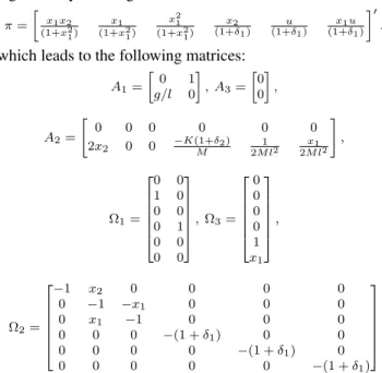
The system (33) can be represented in its differential-algebraic by defining
π= »
x1x2 (1+x2 1)
x1 (1+x2
1) x2
1 (1+x2
1) x2 (1+δ1)
u (1+δ1)
x1u (1+δ1)
–′
. which leads to the following matrices:
A1=
» 0 1 g/l 0 –
, A3=
» 0 0 –
,
A2=
"
0 0 0 0 0 0
2x2 0 0 −K(1+M δ2) 1 2M l2
x1 2M l2
#
,
Ω1=
2 6 6 6 6 6 4 0 0 1 0 0 0 0 1 0 0 0 0 3 7 7 7 7 7 5
,Ω3=
2 6 6 6 6 6 4 0 0 0 0 1 x1 3 7 7 7 7 7 5 ,
Ω2=
2 6 6 6 6 6 4
−1 x2 0 0 0 0
0 −1 −x1 0 0 0
0 x1 −1 0 0 0
0 0 0 −(1 +δ1) 0 0
0 0 0 0 −(1 +δ1) 0
0 0 0 0 0 −(1 +δ1)
3 7 7 7 7 7 5
Similarly, the SFL control law as presented in (32) can be represented as in (5) by taking
w= »
x1 (1+x2
1) x2
1 (1+x2
1) x2 (1+x2
1)
x1x2 (1+x2 1)2
x1 (1+x2
1)2 x2
1 (1+x2
1)2
–′
and
B1=
» 0 0 –′
, B2=
2 6 6 6 6 6 4
2M l2(k 1−g/l)
0 2M l2(k
2+K/M)
−4x2M l2
0 0 3 7 7 7 7 7 5 ′ ,
ζ1=
2 6 6 6 6 6 4 1 0 0 0 0 1 0 0 0 0 0 0 3 7 7 7 7 7 5
, ζ2=
2 6 6 6 6 6 4
−1 −x1 0 0 0 0
x1 −1 0 0 0 0
0 −x2 −1 0 0 0
0 0 0 −1 x2 0
1 0 0 0 −1 −x1
0 0 0 0 x1 −1
3 7 7 7 7 7 5 (34)
For illustrative purposes, in this example we consider the fol-lowing bounds on the statesx1andx2:
|x1| ≤0.15, |x2| ≤0.15
and the parameters considered in the numerical experiments are given in Table 1.
Solving Theorem 4 (taking the Remark 1 into account) and performing a griding search in the uncertainties δ1 andδ2,
we have obtained the following bounds on the uncertain pa-rameters
|δ1| ≤0.097 and |δ2| ≤0.99,
and the following estimate of the domain of attraction
D=
x:x′
62 33 33 64
x≤1
.
Table 1: Pendulum Parameters
Parameter Value
M 2 kg
l 1 m
g 9.8 m/s2
K 0.5 N.s/m
k1 -1
k2 -2
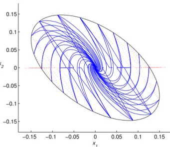
To check the accuracy of these results, several simulations have been performed for a set of initial conditions satisfying
V(0) = 1and at the extremum values ofδ1andδ2leading to
four trajectories for each initial condition. Figure 1 shows the polytope of admissible statesX, the estimate of the domain of attractionD and the stable system trajectories (obtained through simulations).
−0.15 −0.1 −0.05 0 0.05 0.1 0.15
−0.15 −0.1 −0.05 0 0.05 0.1 0.15 x 1 x 2 X
Figure 1: Domain of Attraction and Phase Trajectories.
We have also made an analysis of conservativeness by in-creasing the bound onδ1and testing the system trajectories
if they converge or not to the equilibrium point. We have noted that forδ1≥0.102the system trajectories do not
con-verge to the equilibrium point under analysis as illustrate in Figure 2, where the red dotted lines represent unstable tra-jectories. It turns out this value is only 5 % larger than the estimated bound onδ1demonstrating that the method is not
−0.15 −0.1 −0.05 0 0.05 0.1 0.15 −0.15
−0.1 −0.05 0 0.05 0.1 0.15
x
1
x
2
Figure 2: Phase trajectories forδ1= 0.102.
5
CONCLUSIONS
The paper has presented a methodology to the stability anal-ysis of uncertain nonlinear systems subject to a state feed-back linearization control law. Through a suitable system and control law decompositions, we devise LMI conditions that ensure the local asymptotical stability of the uncertain system while providing an estimate of the system domain of attraction based on quadratic Lyapunov functions. In addi-tion, we can estimate the set of admissible uncertainties via a line search on the parameter bounds. The approach have been applied to the stability analysis of an inverted pendulum system subject to a stabilizing feedback linearization control demonstrating the applicability of the proposed results. We emphasize the results derived in this paper can be easily ex-tended to deal with multi-input multi-output feedback lin-earizing schemes, and, currently, the authors are extending the methodology to deal with actuator saturation.
REFERENCES
Boyd, S., El Ghaoui, L., Feron, E. and Balakrishnan, V. (1994).Linear Matrix Inequalities in System and Con-trol Theory, SIAM.
Chesi, G., Garulli, A., Tesi, A. and Vicino, A. (2004). Robust analysis of LFR systems through homogeneous polyno-mial Lyapunov functions,IEEE Transactions on Auto-matic Control49(7): 1211–1215.
Coutinho, D. and Danes, P. (2006). Piecewise Lyapunov functions to the stability analysis of rational systems subject to multiple state constraints, Proc. 45th IEEE Conference on Decision and Control, pp. 5801–5806.
Coutinho, D. and Fu, M. (2002). Guaranteed cost con-trol of uncertain nonlinear systems via polynomial lya-punov functions,IEEE Transactions on Automatic Con-trol47(9): 1575–1580.
Coutinho, D., Fu, M., Trofino, A. and Danes, P. (2008). L2
-gain analysis and control of uncertain nonlinear sys-tems with bounded disturbance inputs, International Journal of Robust and Nonlinear Control 18(1): 88– 110.
Coutinho, D., Pagano, D. and Trofino, A. (2004). On the esti-mation of robust stability regions for nonlinear systems with saturation,Controle & Automação15: 269–278.
Coutinho, D. and Silva Jr, J. d. (2007). Estimating the Re-gion of Attraction of Nonlinear Control Systems with Saturating Actuators,Proc. American Control Confer-ence, pp. 4715–4720.
Coutinho, D., Souza, C., Barbosa, K. and Trofino, A. (2009). Robust linear H∞filter design for a class of uncertain
nonlinear systems: an LMI approach,SIAM Journal on Control and Optimization48(3): 1452–1472.
Danès, P. and Bellot, D. (2006). Towards an LMI approach to multicriteria visual servoing in robotics, European Journal of Control12(1): 86–110.
El Ghaoui, L. and Scorletti, G. (1996). Control of rational systems using linear-fractional representations and lin-ear matrix inequalities,Automatica32(9): 1273–1284.
Franco, A., Bourles, H., De Pieri, E. and Guillard, H. (2006). Robust nonlinear control associating robust feedback linearization and H∞ control, IEEE Transactions on Automatic Control51(7): 1200–1207.
Guillard, H. and Bourles, H. (2000). Robust feedback lin-earization, Proc. 14 th International Symposium on Mathematical Theory of Networks and Systems.
Hahn, J., Mönnigmann, M. and Marquardt, W. (2008). On the use of bifurcation analysis for robust controller tun-ing for nonlinear systems,Journal of Process Control
18(3-4): 408–420.
Isidori, A. (1995). Nonlinear Control Systems, Springer.
Khalil, H. (2002). Nonlinear systems, Prentice Hall, Upper Saddle River.
Kiyama, T. and Iwasaki, T. (2000). On the use of multi-loop circle criterion for saturating control synthesis,Systems & Control Letters, Vol. 41, pp. 105–114.
Papachristodoulou, A. and Prajna, S. (2004). Analysis of non-polynomial systems using the sum of squares de-composition,Positive Polynomials in Control, Springer
.
Park, C. (2003). LMI-based robust stability analysis for fuzzy feedback linearization regulators with its appli-cations,Information Sciences152: 287–301.
Silva Jr, J. d., Tarbouriech, S. and Reginatto (2004). Applica-tion of hybrid and polytopic modelling to the stability analysis of linear systems with saturating inputs, Cont-role & Automação15: 401–412.