i
Gigliotti Angelo
EXTRACTING TEMPORAL AND SPATIAL DISTRIBUTIONS
INFORMATION ABOUT MARINE MUCILAGE PHENOMENON
BASED ON MODIS SATELLITE IMAGES
ii
EXTRACTING TEMPORAL AND SPATIAL DISTRIBUTIONS
INFORMATION ABOUT MUCILAGE PHENOMENON BASED
ON MODIS SATELLITE IMAGES
A Case of Study for Italy Seas, 2010-2012
Dissertation supervised by
Professor Mário Caetano, PhD.
Instituto Superior de Estatística e Gestão de Informação
Universidade Nova de Lisboa
Lisbon, Portugal
Dissertation co-supervised by
Professor Marco Painho, PhD.
Instituto Superior de Estatística e Gestão de Informação
Universidade Nova de Lisboa
Lisbon, Portugal
Dissertation co-supervised by
Professor Filiberto Pla, PhD.
Departamento de Lenguajes y Sistemas Informatícos
Universitat Jaume I
Castellón, Spain
iii
ACKNOWLEDGEMENTS
I would like to express my deep gratitude to Prof. Mário Caetano, my research supervisor, for his patient guidance, valuable comment and useful critiques of this research work. My grateful thanks are also extended to Prof. Marco Painho my co-supervisor for his advice and assistance in keeping my progress on schedule and his support for us throughout the entire Geospatial Technologies Master’s Program. I would like to also thank to Prof. Filiberto Pla for their co-supervision of this study.
I would also like to extend my thank to the following agency for their assistance with the collection of my data: NASA Land Processes Distributed Active Archive Center (LP DAAC), USGS/Earth Resources Observation, Regional Agency for Environmental Protection and Prevention of the Veneto (ARPAV) and of the Campania (ARPAC).
Special thanks goes to Prof. Dr. Marco Painho, Dr. Christoph Brox and all
concerning person’s for providing all the facilities and for executing this master
program successfully. Equally I would also like to thank to all the staff member of ISEGI and IFGI.
I would like to thank all the people with whom I had the pleasure of sharing my hours of work and life in these last 18 months. In particular I would like to thank my friends and colleagues Stefan and Helder for their suggestions and good company during the thesis work and in the master. I would like to thank Lia that has proceeded to review the translation of my thesis work. I also like thanks my flatmates Silvio and Martina for their support and patience. I would like thanks Concetta and Marco that have been my family in Lisbon. I would like thank my friends Vanessa and Gunnar for making me feel at home in the middle of the westfalia. I would also like thank my collegue Riazzudin, Alberto, Roberto, Diego and Ardit for their friendship and availability during the rest of the master.
iv
EXTRACTING TEMPORAL AND SPATIAL
DISTRIBUTIONS INFORMATION ABOUT MARINE
MUCILAGE PHENOMENON BASED ON MODIS
SATELLITE IMAGES
A Case of Study for Tyrrhenian and the Adriatic Seas, 2010-2012
ABSTRACT
A novel approach was used with data from the Moderate Resolution Imaging Spectroradiometer (MODIS) to detect Marine Mucilage in tow different marine areas of the Italy (Campanian Seas and North Adriatic Sea) from 2010 to 2012. The approach involves first deriving a Mucilage Index (MI) based on the medium‐resolution (500 m) MODIS reflectance data correction of the ozone/gaseous absorption and Rayleigh scattering effects and then objectively determining the MI threshold value (0.05<MI<0.45) to separate the Marine Mucilage from other interference. The dynamic feature of time and space can be obtained for the two areas of study using extracted method. Variation of mucilage bloom in these areas is analyzed and discussed in different temporal scale. The mucilage bloom frequency index (MFI) is important criterion which can show the interannual and inter-monthly variation in the whole areas of Campanian Sea and North Adriatic Sea. Utilizing the MFI from 2010 to 2012, it found some phenomena that: thare is an increase of Mucilage formation in the last tree years in the Campanian seas, al contrario in
v
KEYWORDS
Remote Sensing
Oceanography
Marine Pollution
MODIS
Sea Surface Temperature
Mucilage Bloom
Mediterranean Sea
vi
ACRONYMS
AVHRR
Advanced Very High Resolution Radiometer
NASA
National Aeronautics and space administration
SST
Sea Surface Temperature
LP DAAC
Land Processes Distributed Active Archive Center
MODIS
Moderate Resolution Imaging Spectroradiometer sensor
MRT
MODIS Reprojection Tool
QA
Quality Assessment
QC
Quality Control
RS
Remote Sensing
vii
TABLE OF CONTENTS
ACKNOWLEDGEMENTS...iii
ABSTRACT...iv
KEYWORDS...v
ACRONYMS...vi
TABLEOFCONTENTS...vii
INDEXOFTABLES...ix
INDEXOFFIGURES...x
1.INTRODUCTION ... 1
1.1 Research objectives ... 2
1.2 Study area ... 3
2.1.LITERATURE REVIEW ... 5
2.1.Marine mucilage ... 5
2.1.1.What they are and how they form... 5
2.1.2.Where and when form ... 8
2.2.Meteo-climatic factors influence upon mucilage formation and dispersion ... 10
2.3.Remote sensing and mucilage detection ... 13
2.4.The mucilage index ... 14
3.DATA AND METHODS ... 17
3.1.Satellite data ... 17
3.2.Field data ... 19
3.3.Data acquisition and pre-processing ... 19
3.3.1.Quality correction ... 21
3.4.The mucilage index application ... 23
3.4.Mucilage index threshold ... 25
viii
4.RESULTS AND DISCUSSION ... 31
4.1.Spatial and temporal distribution of mucilage phenomenon ... 31
4.1.1.Annual mucilage frequency index ... 31
4.1.2.Mounthy mucilage frequancy index. ... 36
4.1.3.Sea temperature influence on marine mucilage formation. ... 41
4.2.The 2012 bloom event in campanian sea. ... 43
5.CONCLUSION ... 49
BIBLIOGRAPHIC REFERENCES ... 50
APPENDICES ... 58
APPENDIX 1- In the first column are the digital number chosen as admissible quality. In the second column are the correspondent binary number. ... 59
APPENDIX 2- Dataset of in situ data from ARPAC. ... 61
APPENDIX 3– MODIS Surface reflectance L2G 500 m used in the study and summary quality description. ... 62
ix
INDEX OF TABLE
Table 1- Description and images of the macroaggregate types observed in the Northern Adriatic Sea (Precali et al. 2005). ... 6 Table 2- Science data sets for MODIS Terra Surface Reflectance Daily L2G 500m SIN Grid
V005 (MOD09GA) ... 18 Table 3- 500-meter QA Descriptions (32-bit) ... 22 Table 4- The total days of the status of monitoring mucilage bloom using MODIS image in
x
INDEX OF FIGURES
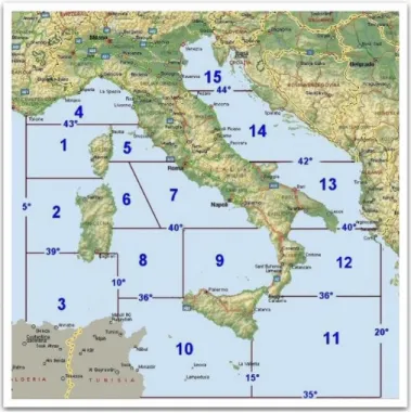
Figure 1– Corsican Sea, 2-Sardinian Sea, 3-Strait of Sardinia, 4-Ligurian Sea, 5-N. Tyrrhenian Sea, 6-7 C. Tyrrhenian Sea (W,E), 8-9 S. Tyrrhenian Sea (W,E) 10 - Strait of Sicily, 11-5. Ionian Sea,
12-N. Ionian Sea, 13-S. Adriatic Sea, 14-C. Adriatic Sea, 15-N. Adriatic Sea... 4
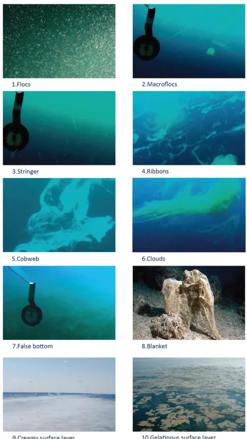
Figure 2– Classification of different Mucilages aggregates (Precali et al. 2005). ... 7
Figure 3- Formation of a false bottom at the picoclinio verified by observations with camera subacquea and ecoscandiglio (Giani et al, 2005). ... 8
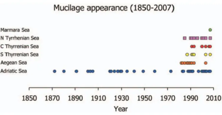
Figure 4- The areas in the Mediterranean Sea where the mucilage has been documenteand the years of appearance. (R. Denovaro et al., 2009) ... 9
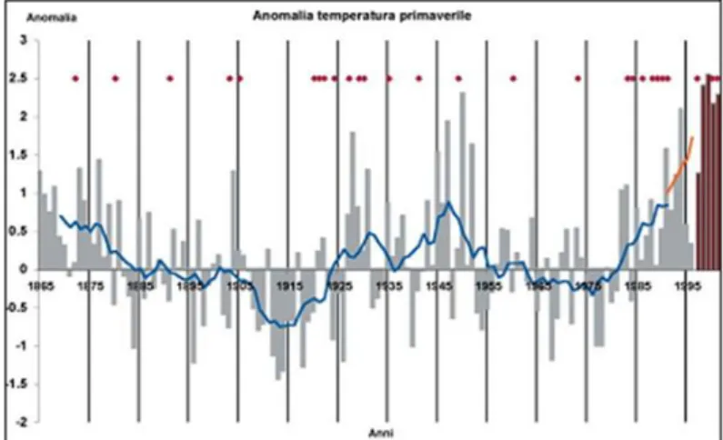
Figure 5- Trend anomaly of mean temperature of the air spring to the Po Valley area used for comparison with the episodes of mucilage occurred during the summer. Also shows the moving average of the weather variable calculated on 10 years. (Deserti M. et al, 2003). ... 11
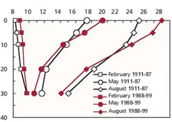
Figure 6- Comparison between the monthly mean temperature profiles (February, May, August) obtained using data prior to 1987 (black line) with those obtained using the data after this year (red line) (Russo et al., 2003). ... 12
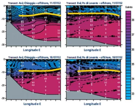
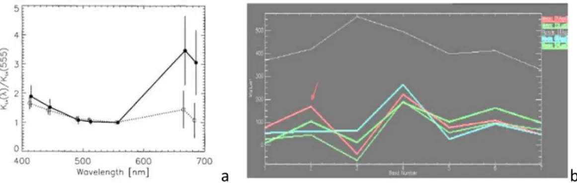
Figure 7–In the left: Average spectra of the diffuse attenuation coefficient for upwelling radiance, Kλu, normalized to the value at 555 nm, computed for 1m thick layers, for two different dataset (Berthon et al. 2000). In the right: MODIS spectral signature of the filaments observed in Adriatic Sea. In 23, 24 July, 1 and August 5, 2002. The values are lower than those of clouds on the sea August 1 (curve high) (Vescovi et al., 2003). ... 15
Figure 8- Calibration curve of the satellite signal from data observed at sea (Vescovi et al., 2003). .. 16
Figure 9- Mucilage Event of 7 July 2004, North Adriatic Sea (Vescovi et al., 2003) ... 16
Figure 10- A global representation of standard MODIS land product tiles. ... 20
Figure 11– The workflow created with the ArcGIS Model Builder illustrates a graphical environment in which the different data sources used in this study (represented in dark blue circles) are connected to the operations previously descripted (represented in brown boxes) and chained through the outputs (new data represented in Green circles). ... 24
Figure 12– Histogram of validation result using ARPAC in situ dataset. ... 25
Figure 13– Histogram of validation result using ARPAV in situ dataset. ... 26
Figure 14– Box-plot of validation data and common errors using MI. ... 27
Figure 15– The workflow created with the ArcGIS Model Builder illustrates a graphical environment in which one entire dataset is processed through iteration of the same operation to produce the images of Mucilage detection. ... 28
Figure 16- Selected areas for Spatio Temporal Analisis of Mucilage phenomenon in the summer of 2010, 2011 and 2012. ... 30
Figure 17– The Annual Mucilage Frequency Index from 2010 until 2012 in South Tyrrhenian (Campania) and North Adriatic Sea (Veneto). ... 32
Figure 18- The spatial distribution patterns of the annual mucilage frequency index in Campania sea ... 34
Figure 20–The spatial distribution patterns of the month mucilage frequency index in Campania seas. ... 36
Figure 21– The spatial distribution patterns of the month mucilage frequency index in Campania seas. 2012 ... 38
Figure 22– The spatial distribution patterns of the month mucilage frequency index in North Adriatic seas. ... 38
Figure 23- The spatial distribution patterns of the month mucilage frequency index in North Adriatic seas. 2012 ... 39
Figure 24- The month Mucilage Frequency Index in the summer season from 2010 until 2012 in South Tyrrhenian (Campania) ... 40
xi
Figure 26– Monthly mean of Sea Temperature in Veneto. The Value are collepted from ISPRA stations of Venice... 42 Figure 27- The Scatter plots in Figure showing the relationship between two variables of MAFI and
Monthly mean sea temperature. ... 43 Figure 28- extensive mucilage bloom reported by ARPAC in July 03, 2012
(http://www.arpacampania.it/balneazione/a_mucillagini2012_relazioni_sopralluoghi.asp et) occurred in Centola (South of Salerno Province) ... 44 Figure 29- The sequence of figure describe a massive mucilage phenomeno in the summer of 2012 in Campanian seas by the use of Mcilage Index (MI). (Junrato 15-Jul 14) ... 45 Figure 30- The sequence of figure describe a massive mucilage phenomeno in the summer of 2012 in Campanian seas by the use of Mcilage Index (MI). (Jul 17 – Aug 2) ... 46 Figure 31- extensive mucilage bloom reported by ARPAC in July 11, 2012
(http://www.arpacampania.it/balneazione/a_mucillagini2012_relazioni_sopralluoghi.asp et) occurred in Trentaremi bay (Golf of Naples) ... 47 Figure 32- Extent (in Km2) of Mucilage phenomenon in Campania Region during summer 2012. ... 48
1
1.
Introduction
Marine pollution is a serious global problem, especially in developing countries where excessive nutrients and other pollutants from rapidly growing agriculture, aquaculture, and industries are delivered to lakes, estuaries, and other coastal waters. As a result, coastal resources are under perceptible stress, with significant degradation in water quality, biodiversity, and fish abundance. In this condition most of seas areas are being affected increasingly and frequently by large scale phenomena of marine pollution (Cracknell et al., 2001).
One of the most discussed in the last two decades with regard to the Mediterranean Sea and in particular the Italian coast is the phenomenon of Marine Mucilage. These phenomena are characterized by rapid and excessive growth of amorphous aggregates of gelatinous material consist mostly by transparent exopolymeres particles (TEP) and organic matter (Aldredge, 1999).
The phenomenon of mucilage on the Italian coast is not at all new. The first reports about the presence of mucilaginous material on the Italian coasts date back to 1729 (Bianchi 1746) in the Adriatic Sea, one of the most severely affected area, and have taken place at various times from 800 to the present day. In the last decades this phenomenon shows itself more and more frequently, but with variable intensity, alternating periods of mass production with years of almost total absence (Giani et al, 2003).
2
water column and high water temperatures, in fact the appearance of mucilaginous material occurs above all in the summer months from June to September (Penna et al., 2003).
A part from Their intrinsic scientific interest, Their Importance lies in the fact that mucilage aggregate can have a negative impact not Also on the biocenosis of the seabed, but also on human productive activities related to tourism and fisheries (The European Union has compensated the Italian fishing for as many as 29 million euro for the fishing ban caused by mucilage in the Adriatic Sea in the summer of
2000 (Ecoharm 2003)), and although there are no reports of cases with negative consequences for human health, produced by contact with the mucilage (Funari & Ade, 1999), we cannot be completely ruled out, in polluted areas, health-related implications for bathing.
In this context, it appears really important to establish monitoring and forecasting tools, through which observe and investigate this type of large scale phenomenon. Over recent years the mucilage formation is monitored by some Environment Regional Agencies and Italian research institutes. However, this duty has been traditionally undertaken, through a series of 'in situ' monitoring programs with increasing frequency at the main algal bloom season. Under this perspective, Remote Sensing has the potential to provide greater spatial coverage, greater temporal coverage and additional environmental information (Fischer, 1985).
1.2. Research objectives
The overall objective of this Research based on MODIS remote sensing data is the study and monitoring of mucilage phenomenon in the Mediterranean Sea in particular with regard to the Italy coasts.
3
- Establishes method and technology to extraction the time and space distribution information of Mucilage Bloom.
- Based on extracted information and index, obtaining the dynamic feature of time and space in the Italian coasts from 2010 to 2012.
- Analyses and discusses variation of mucilage bloom in the Italy coasts during this time.
1.3. Study area
The study area includes all the Italian seas. As shown in figure 1 this area is located in the middle of the Mediterranean Bacin between latitudes 35 ° and 47 ° N, and Longitudes 5 ° and 20 ° E, in WGS84. The air study includes all the Italian seas. As shown in figure this area is located in the middle of the Mediterranean Bacine between latitudes 35 ° and 47 ° N, and Longitudes 5 ° and 20 ° E, in WGS84.
Each of these seas has different characteristics of depth, salinity, temperature, transparency, currents and tides. As for the rest of the Mediterranean, the surface temperature of the Italian seas is on average rather high. In the northern Tyrrhenian, the Sea of Sicily, Ionian and southern Adriatic it is about 13 º, in the Ligurian Sea about 12 º, in the southern Tyrrhenian about 14 º, but in the northern Adriatic, Because of the shallowness of the waters, it drops to 9 º. The Italian seas are also characterized by a high salinity, between 37.70 ‰ and 38.50 ‰, with lows of 32.70 ‰ due to insufficient riverine inputs of freshwater, moderate currents and
4
5
2.1
Literature review
2.1. Marine mucilage
2.1.1. What they are and how they form
6
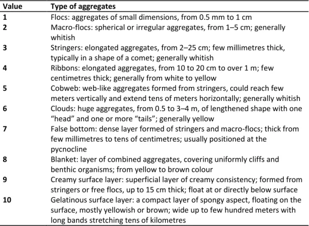
stratification of the water column, high diatom biomass, and the dominance of these species (Passow et al., 1995). The aggregates may have a very different size and morphology, and they have therefore been classified according to their structural form and their spatial arrangement along the water column (Stachowitsch et al., 1990; Precali et al., 1999). The different types (Figure 2) are briefly described in Table 1.
Value Type of aggregates
1 Flocs: aggregates of small dimensions, from 0.5 mm to 1 cm
2 Macro-flocs: spherical or irregular aggregates, from 1–5 cm; generally whitish
3 Stringers: elongated aggregates, from 2–25 cm; few millimetres thick, typically in a shape of a comet; generally whitish
4 Ribbons: elongated aggregates, from 10 to 20 cm to over 1 m; few centimetres thick; generally from white to yellow
5 Cobweb: web-like aggregates formed from stringers, could reach few meters vertically and extend tens of meters horizontally; generally whitish
6 Clouds: huge aggregates, from 0.5 to 3–4 m, of lengthened shape with one
“head” and one or more “tails”; generally yellow
7 False bottom: dense layer formed of stringers and macro-flocs; thick from few millimetres to tens of centimetres; usually positioned at the
pycnocline
8 Blanket: layer of combined aggregates, covering uniformly cliffs and benthic organisms; from yellow to brown colour
9 Creamy surface layer: superficial layer of creamy consistency; formed from stringers or free flocs, up to 15 cm thick; float at or directly below surface
10 Gelatinous surface layer: a compact layer of spongy aspect, floating on the surface, mostly yellowish or brown; wide up to few hundred meters with long bands stretching tens of kilometres
Table 1-Description and images of the macro-aggregate types observed in the northern Adriatic Sea (Precali et al. 2005).
7
8
2.1.2 Where and when form.
Aggregates, particularly large ones, tend to accumulate in the frontal areas of contact between the pelagic and coastal waters, or in correspondence of density gradients due to seasonal thermal stratification and the contributions of freshwater river (Giani et al, 2005).
Figure 3- Formation of a false bottom at the picoclinio verified by observations with camera subacquea and ecoscandiglio (Giani et al, 2005).
9
Adriatic Sea; on the contrary, in other Italian seas, such as the Tyrrhenian Sea, even if specific studies on this issue are limited, it has been reported as a phenomenon on basin scale. Some areas of the Adriatic, such as the Kvarner bay and the central area between the Po delta and Istria, appear to be favourable to the genesis and development of the aggregates (Precali et al., 2005). The phenomenon generally occurs, at first, along the Istrian and Dalmatian costs and, subsequently, along the Italian coasts, affecting sometimes the Central and South Adriatic.
One of the first observations concerning the outcrop of gelatinous masses on large surfaces, dates back to 1729 in the Adriatic Sea (Bianchi, 1746), but the first scientific description refers only to 1872. Similar phenomena were observed in the years 1880, 1891, 1903, 1905, 1920, 1949 (Figure), as documented by collecting reports of the time (Human Fonda et al., 1989). Then there are outcrops only in limited areas, such as in 1973, in the Kvarner (Zavodnik, 1977), in 1983, in the Gulf of Trieste and the Dalmatian island of Krk (Stachowitsch, 1984) along with an anoxic crisis in 1984, in various parts of the northern and southern Adriatic (Vilicic, 1991), in 1986, in the Kvarner (Herndl & Peduzzi, 1988) and in 1990, and in the Kvarner area near the coasts of Emilia Romagna (Andreoli et al., 1992). Studies in the last two decades show that this phenomenon shows itself more and more frequently, but with variable intensity, alternating periods of mass production with years of almost total absence (Giani et al, 2003).
10
2.2. Meteo-climatic factors influence upon mucilage formation and
dispersion.
11
accumulation of such water also affects, in addition to the availability of nutrients vehicled, the stability of the water column due to density gradients that are created between the hot water and less salted surface waters and dense background, saltier and colder. Some studies demonstrate how some season’s rich mucilaginous
phenomena have been characterized by a prior increase in stability of the water column (Degobbis et al., 2000). Finally, as regards temperature, spectral analysis of time series of temperature anomaly spring and the presence / absence of mucilage on meteorological data for northern Italy, in general, and some stations Adriatic, in
particular, seems to indicate a correlation between the positive anomalies and events of mucilage, which occur common with frequencies of about 6 and 3 years. However, in evaluating these results must take into account the relative limitation of extension of the time series and the uncertainty in the definition of the events of mucilage. This definition includes all the events reported and should be considered that the grouping into clusters is less clear if we take into account only the events considered to be certain documented (Giani M, 2002). Trend anomaly of mean temperature of the air spring to the Po Valley area used for comparison with the episodes of mucilage occurred during the summer. Also shows the moving average of the weather variable calculated on 10 years. (Deserti M. et al, 2003).
12
For the last period of positive anomaly (i.e. increase with respect to the average), atmospheric temperature has also been verified an increase in sea surface temperatures of the Adriatic basin, while the deep have not changed or even show a slight decrease in the value of temperature. Therefore, the second half of the '80s, the northern Adriatic basin is characterized by a vertical temperature gradient more pronounced, which probably increased the stability conditions of the water column (Russo et al., 2003).
Figure 6-Comparison between the monthly mean temperature profiles (February, May, August)
obtained using data prior to 1987 (black line) with those obtained using the data after this year (red line) (Russo et al., 2003).
13
temperature (Thornton & Thacke, 1998). Another effect of temperature is to increase so exponential the benthic respiration facilitating the formation of hypoxia and anoxia, which may be aggravated by the sedimentation of organic material present in the mucilaginous aggregates (Herndl et al., 1989).
2.3. Remote sensing and mucilage detection
Satellite remote sensing provides rapid, synoptic, and repeated information on water state variables (physical and bio-geochemical) that avoids interpretive problems associated with under sampling. Indeed, over the last three decades, there have been significant advances in technology and algorithm development allowing satellite ocean colour measurements to be used for studying coastal ocean water quality. Most of these advancements have focused on turbidity, water clarity, or other bio‐optical properties (Dekker, 1993; Hu et al., 2004; Chen et al., 2007, Lee
14
foresaw the creation of a network for the collection and integration of information concerning the eutrophication and mucilage phenomenon of waters of the central and northern Adriatic, collected by environmental regional agencies and research
institutes from Croatian and Italian
(www.regione.emiliaromagna.it/pda/iiia_requisite_eng.htm). In this context, it is developed the work of the Remote Sensing laboratory of ARPA SMR in which a detection algorithm is implemented to identify the mucilage index through the use of MODIS Surface Reflectance product (Vescovi et al. 2003). The mucilage Index was
used for the mapping of mucilage events occurred in the summer of 2004 (ARPA, 2005). However, to the best of my knowledge there are no more examples in literature on the application of mucilage index or implementations of new products for the automatic detection. Remain therefore limited information on the presence, extension and temporal evolution of mucilaginous phenomena about affected areas, with the exception of in situ observations made by the regional environmental protection agencies and news from the press agency.
2.4. The Mucilage Index.
The Mucilage Index from Mucilage phenomenon detection in The Nord Adriatic Sea defined by Vescovi et al. (2003) is descript by the follow equation:
M = (((B2 + B4)/2) - B3)/B6 (1)
B2 = Surface Reflectance Band 2 (841 - 876 nm)
B3 = Surface Reflectance Band 3 (459 - 479 nm)
B4 = Surface Reflectance Band 4 (545 - 565 nm)
15
The numerator of the formula enhances the decrease of reflectance typical of mucilaginous material in the channel 3 compared to the average values of the channels 2 and 4. The low reflectance in the band 3 (459-479 nμ) and the highest reflectance in band 4 (545-565 nμ) are confirmed by measurements in situ with radiometers made in previous studies (Berthon al. 2000)(Figure 7a). Furthermore, also the studies carried out by Tassan (1993) with sensor NOAAAVHRR confirm that in the near infrared wavelength, corresponding to the band 2 of the MODIS (841-876 nμ), the reflectance of this material is greater. The channel 6 in the formula is at
the denominator because it usually has a very high value in case of the clouds and very low in case of mucilage. The formula, therefore, enhances the optical properties of the mucilage and discriminates the clouds, which could constitute the first element of confusion with the mucilage bodies as they also are very clear and sometimes filamentous case of stripes left by the aircraft (Vescovi et al., 2003).(Figure 7b)
a b
Figure 7–In the left: Average spectra of the diffuse attenuation coefficient for upwelling radiance,
Kλu, normalized to the value at 555 nm, computed for 1m thick layers, for two different dataset
(Berthon et al. 2000). In the right: MODIS spectral signature of the filaments observed in Adriatic Sea. In 23, 24 July, 1 and August 5, 2002. The values are lower than those of clouds on the sea August 1 (curve high) (Vescovi et al., 2003).
16
Figure 8 -Calibration curve of the satellite signal from data observed at sea (Vescovi et al., 2003).
17
3
.Data and methods
3.1. Satellite data
In this study we used satellite images from MODIS sensors. MODIS (Moderate Resolution Imaging Spectroradiometer) is a land, ocean, and lower atmosphere observing instrument. It is aboard the Terra (EOS AM) and Acqua (EOS PM) satellites that are part of NASA’s Earth Observing System (EOS) established for long term observations of the Earth’s biosphere. MODIS acquires images from every point on Earth at least once every 1 or 2 days. It covers the visible to the near infrared (0.4- 1.4 um) spectrum with 36 spectrum channel and its scanning width is 2330 km, whose spatial resolution is 250m, 500m and 1000 m and the temporal resolution is twice a day. Science teams have developed a variety of standard data products which are distributed free of charge by the Land Processes Distributed Active Archive Centre. (NASA 2009).
18
3.1.1. The Surface Reflectance products
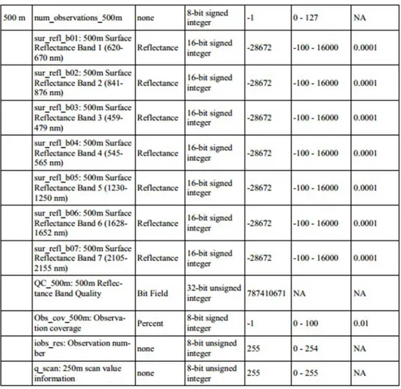
The MODIS Surface Reflectance products provide an estimate of the surface spectral reflectance as it would be measured at ground level in the absence of atmospheric scattering or absorption. In particular for this study we used MOD09GA product. The MOD09GA provides Bands 1-7 in a daily gridded L2G (Level 2) product in the Sinusoidal projection, including 500-meter reflectance values and 1 kilometre observation and geo-location statistics. The product also contains data sets
describing cloud cover and data quality for each pixel (Table 2) (EODIS, 2009).
19
3.2. Field data
Many field sampling data have recorded and documented the events of Mucilage blooms in coastal waters around Italy, for the summer seasons of the years 2010, 2011 and 2012 (Table). They are collected from different regional environmental agency of Italy (ARPA), with not standardized mode. The majority of these is the result of chemical, physical and biological measurements. Fortunately, thanks to the work carried out by ARPA Campania (ARPAC) following the mucilaginous exceptional events occurred in the summer 2012 on the Campania coasts we have also a useful photographic documentation of the most important events, including geographic location, extension and state of aggregation (APPENDIX2)(www.arpacampania.it/balneazione/a_mucillagini2012_relazioni_sopr alluoghi.asp). We subsequently used this data to calibrate and validate the product derived from satellite images. Another Dataset from ARPA Veneto (ARPAC), originated from video-observations of underwater marine monitoring stations it
was also used to compared the different source
(http://www.arpa.veneto.it/bollettini/htm/qualita_acque.asp?a).
3.3 Data acquisition and pre-processing
The Land Processes Distributed Active Archive Center (LP DAAC) stores a variety of MODIS land products in standard 10º x 10º tiles in Sinusoidal projection and HDF-EOS format (Figure 10).
20
able to spatial subsetting, band subsetting, re-projecting, resampling, and reformatting all the images before to downloading.
Figure 10- A global representation of standard MODIS land product tiles.
We downloaded daily images for the summer period (01 Jun - 31 September) of tree years (2010 - 2012). To avoid cloud‐induced bias in the area coverage statistics, only when the study area contained at least 75% cloud‐free data were those data extracted and analysed (APPENDIX 3).We selected for each day 6 layer used in the analysis, Band 1, Band 2, Band 3, Band 4, Band 6 and 500m Reflectance Band Quality.
21
3.3.1. Quality correction
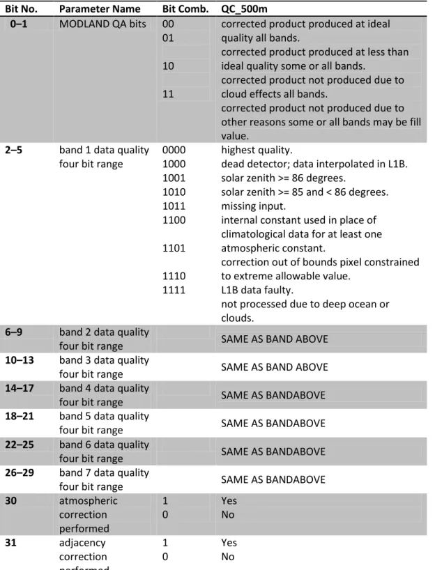
All Modis products include quality assurance (QA) Informations. This information are produced by the MODIS Land Science Team (MODLAND) that is responsible for the MODIS land products in terms of their QA and validation. MODIS QA information provides vital clues regarding the usability and usefulness of the data products for any particular science application. At Pixel level QA provides information for each science parameter through the binary representation of bit combinations that characterizes particular quality attributes defined in MODIS LST Products Users Guideline (Wan 2009). For MOD09GA it was available the QC_500m Reflectance Band Quality product which the quality information is stored in 32 bit integer with a valid range of (0-4294966019) (Vermote et Al., 2002).
22
Bit No. Parameter Name Bit Comb. QC_500m 0–1 MODLAND QA bits 00
01
10 11
corrected product produced at ideal quality all bands.
corrected product produced at less than ideal quality some or all bands.
corrected product not produced due to cloud effects all bands.
corrected product not produced due to other reasons some or all bands may be fill value.
2–5 band 1 data quality four bit range
0000 1000 1001 1010 1011 1100 1101 1110 1111 highest quality.
dead detector; data interpolated in L1B. solar zenith >= 86 degrees.
solar zenith >= 85 and < 86 degrees. missing input.
internal constant used in place of climatological data for at least one atmospheric constant.
correction out of bounds pixel constrained to extreme allowable value.
L1B data faulty.
not processed due to deep ocean or clouds.
6–9 band 2 data quality
four bit range SAME AS BAND ABOVE
10–13 band 3 data quality
four bit range SAME AS BAND ABOVE
14–17 band 4 data quality
four bit range SAME AS BANDABOVE
18–21 band 5 data quality
four bit range SAME AS BANDABOVE
22–25 band 6 data quality
four bit range SAME AS BANDABOVE
26–29 band 7 data quality
four bit range SAME AS BANDABOVE
30 atmospheric
correction performed 1 0 Yes No
31 adjacency
correction performed 1 0 Yes No
23
3.4. The Mucilage Index application.
The processing carried out by us on MODIS data is based on the calculation of the Mucilage Index M, defined by Vescovi et al. (2003).
M = (((B2 + B4)/2) - B3)/B6
B2 = Surface Reflectance Band 2 (841 - 876 nm) B3 = Surface Reflectance Band 3 (459 - 479 nm) B4 = Surface Reflectance Band 4 (545 - 565 nm) B6 = Surface Reflectance Band 6 (1628 - 1652 nm)
Were analysed MODIS images during the time interval June-September of the years 2010, 2011, 2012 and were drawn 296 scenes for a total of 270 cards produced.
Processed Images Not Processed Effective Monitoring
Days
Bad Quality Days Cloudless Days
June 2010 20 1 9
July 2010 24 6 1
August 2010 22 9 -
September 2010
13 3 14
June 2011 20 - 10
July 2011 22 2 7
August 2011 29 1 -
September 2011
21 1 8
June 2012 26 1 3
July 2012 27 1 3
August 2012 30 1 -
September 2012
16 - 14
Total 270 26 69
Note: Effective monitoring day means the days of completing activities of monitoring indicator normally. Cloudless days are the days without cloud cover within the whole Study area in a year (less 75%). Bad Quality Days are the days whit presence of large areas covered by errors that have not been masked by the pre-processing.
24
Some dates are missing due to the presence of excessive errors detected in the data that have not been masked by the pre-processing (Table 4). We performed this check through visual analysis of the images processed by the algorithm and the correspondent True Band Composition (Band 3, Band 1, Band 4) and False Band Composition (Band 2, Band 1, Band 4). These last have been produced for each day of monitoring through Band Composite Tool in ArcGIS.
To automate the processes of analysis described so far we have built a Data processing Model through a Model Builder in ArcGIS (Figure 11). This allowed us to
significantly reduce the Data processing times.
25
3.4. Mucilage Index threshold
The most critical task in distinguishing Mucilage Phenomenon from other waters disturbances (e.g. river sediments) was to determine the threshold value in the Mucilage Index imagery.
In a previous study the mucilage index has been calibrated with in situ data for the area of the Northern Adriatic Sea (see Paragraph 2.4). It was identified a range of values between 0 and 5 that corresponds to the occurrence of mucilage. The study also shows that values below 0.6 exhibited little interference from other substances in the sea (Vescovi et al., 2003). Therefore we decided to keep that value as limit threshold in the beginning stage of our analysis. Unfortunately, visual analysis of the preliminary results revealed that the afore mentioned threshold is not appropriate for the discrimination of mucilage from other interference phenomenon, in particular turbidity and river plume.
Furthermore, sampling values of mucilage index for the points corresponding to actual measurements in situ has been noted as the range of values obtained were for the 93% positive and below the threshold chosen (Figure 12 and 13).
26
Figure 13– Histogram of validation result using ARPAV in situ dataset.
The differences between the mean values of mucilage index obtained from the two different datasets are due to the use of different sampling methods. The data collected by ARPA Campania being sampled directly on the sea surface are considered the most reliable ones.
In order to define the most appropriate limit threshold for the used algorithm and improve the accuracy of the final result we decided to compare the validation result from in situ data with the average value of MI obtained from the most common errors in the images (collected by visual analysis).
27
The results are represented by the use of box plots shown in figure 14
28
The values of the validation dataset exhibit a different range than those of the mentioned error sources: the upper limit of the upper quartile (75th percentile) of the validation datasets lies beyond the lower quartile (25th percentile) of the latter. A small interference can only be observed for clouds as well as the MODIS errors. Consequently, we decided to choose the minimum and Upper Quartile (3rd Qu in Figure 14) from ARPA Campania dataset (0.05<Mucilage Index< 0.45) as threshold for our MI.
Subsequently the maps of mucilage index were reclassified with values equal to
1 for the pixels that have values within our threshold and 0 for the remaining pixels. The results are daily maps of effective mucilage detection.
To automate the processes of analysis for the entire mucilage index database we built a data processing model through model builder in ArcGIS (Figure 15).
Figure 15–The workflow created with the ArcGIS Model Builder illustrates a graphical environment
29
3.5. Spatio-temporal analisis
In order to extract information on spatial and temporal phenomenon of mucilage to the area of study we applied a method used in previous studies for the analysis of spatio-temporal phenomena of eutrophication (Hu et al, 2010; Chunguang et al., 2012), which includes the use of the algal frequency index (AFI).
AFI is defined as the number of the algae bloom days against the number of effective monitoring days marked as T in a certain water area at certain time. Using MODIS data, the size of a certain water area is the 500m*500m, a size of a pixel, and a certain time usually is 365day in a year (Jin Y et al, 2009; Ma et al, 2010). The mathematical expression is as the follow:
AFI = t / T*100% (2)
As the algae bloom study we used AFI to extract spatio-temporal distribution of Mucilage phenomenon.
In order to measure the inter-month variation, a certain time is often set to the days of a month in a year and certain water region is defined as the whole study area or a sub-region. This kind of AFI is called monthly mucilage bloom frequency index (MMFI).
30
To better describe the spatial temporal dynamics of mucilage formation we decide to focus the analysis in two sub-region of the study area:
- The North Adriatic seas, between latitudes 44° 10' and 45°90', and Longitudes 12° and 14 ° E. In correspondence of Venetian coasts.
- The South-Central Tyrrhenian See between latitude 39° 90' and 41° 0', and Longitude 13° 50' and 15°70'. In correspondence of Campanian coasts.
-These two areas show the maximum value of mucilage index in the preliminary step of analysis. Therefore are available for this areas in situ data for the period of study 2010-2012.
-Figure 16-Selected areas for Spatio Temporal Analisis of Mucilage phenomenon in the summer of
31
4. Results and discussion
4.1 Spatial and temporal distribution of mucilage phenomenon
4.1.1 Annual Mucilage Frequency Index
Figures 18 e 19 show the spatial and temporal distribution of mucilage phenomenon (0.05<MI<0.45) in the Tyrrhenian Sea along coast of Campania as well as the North Adriatic Sea.
To avoid cloud‐induced errors in the area coverage statistics, we only considered images that were at least 75% cloud‐free in the desired coast segment for further analysis. Also, some images were excluded due to errors not masked during the process of quality assessment
Looking at the maps of Mucilage Annual Frequency Index along the Campania
32
sections of the Campanian coast in recent years is confirmed by numerous reports from news agencies (www.ansa.it, www.ilmattino.it) and official bodies that are in charge of coast control. Particularly in 2012 the intensification of the mucilage phenomenon was due to the climatic conditions during summer season, which was characterized characterized by poor hydrodynamics of the water body and high surface temperatures (www.arpacampania.it / bathing/mucillagine).
NB: In this case the values of AMFI are expressed as average days of detection for pixels that fall in the considered study areas. The average values were normalized to the number of effective monitoring days per study year.
Figure 17–The Annual Mucilage Frequency Index from 2010 until 2012 in South-Central Tyrrhenian
(Campania) and North Adriatic Sea (Veneto).
33
years, especially at monitoring stations that are about 3500 meters off the coast. A mucilage formation of “considerable dimension” was detected on August 10th 2010 about three miles off the coast of Albarella, in Venice Provence. Unlike along the Campania coast the mucilage phenomenon in the Adriatic Sea occurs as isolated areas also in the open see, whereas in Campania it tends to appear as adjacent areas close to the coast. Suchlike, a persistent mucilage formation with an extension of approximately 30 km² can be observed off the coast of Rovigo province at the estuary of the Po river. Numerous studies conducted in recent years
identified this as one of the most affected areas (Sciarra, 2006; Vescovi et al., 2003; Precali et al., 2005).
34
35
36
4.1.2 Mounthly Mucilage Frequancy Index.
It is necessary to discuss the overall progress of the phenomenon, booming in 2010-2012. The visible-infrared remote sensing is easily affected by clouds and rain, so the days of effective monitoring and days of flowering of mucilage monitoring was very different for each month in 2010, 2011 and 2012 (Table 4). In order to obtain the index comparable to reflect the intermonth variation, the mucilage bloom monthly frequency index (MMFI) was used as the reference standard (Figures 20 and 21). The analysis focuses on the summer months of June, July, August and September because in these months have the greatest concentrations of the phenomenon of Mucilage in the Italian seas (Penna et al., 2003).
The Map in Figure 20, 21, 22 and 23 graphs in 24 and 25 shows the monthly variation of mucilage bloom frequency about 2009, 2010 and 2011 for the Campanian Seas and North Adriatic Seas. We can see that the trend in the four months of monitoring is similar for the three years of sampling in the two selected areas.
Lower values there are in the months of June and September, while the peaks occur in the hottest and less rainy months of July and August. We can clearly see that there are three different stages: operation of low level, rising phase, and fall period. For each season the phenomenon has only a rising phase until reaching a peak of maximum production to then have a decay and sedimentation of the
37
.
38
Figure 21–The spatial distribution patterns of the monthly mucilage frequency index in Campanian seas. 2012
39
40
From the comparison between the two graphs for the monitored areas, we see that the peaks in the two regions are the same for the summers of 2010 (July) and 2011 (August), while in 2012 there is a peak in July in Campania and one in August for the Adriatic. This behaviour could be justified by a possible delay in reaching the maximum temperatures for the North Adriatic than the Tyrrhenian Sea in 2012. Other meteo-climatic factors like difference in hydrodynamics conditions or salinity can determine also this situation.
The more high monthly values were recorded in Campania in July of 2012. For this period it is reported by the press and official reports ARPAC several blooming of considerable size across the Campanian Coast (ARPAC, ilmattino.it). Interesting values also occurred for the month of July in the North Adriatic. In this period focus as the majority of the events documented within the last three years by ARPAV across the Veneto coast. This phenomenon continued in August as described by in situ measurements (ARPAV).
NB: In this case the values of AMFI are expressed as average days of detection for pixels that fall in the considered study areas. The average values were normalized to the number of effective monitoring days per study month.
41
NB: In this case the values of AMFI are expressed as average days of detection for pixels that fall in the considered study areas. The average values were normalized to the number of effective monitoring days per study month.
Figure 25–The monthly Mucilage Frequency Index in the summer season from 2010 until 2012 in
South Tyrrhenian (Campania)
4.1.3 Sea temperature influence on marine mucilage formation.
The study of monthly frequency of mucilage leads to the conclusion that there is some cyclicity in the mucilage phenomenon for the studied areas. The factors of influence on the mucilage formation are still under investigation, however some weather variables were already identified as possible elements of acceleration or deceleration in the dynamics of formation and degradation of that phenomenon (Paragraph 2.2).
42
the achievement of the maximum peak of mucilage we could observe how this happens always in the same month when it reach the maximum peaks of temperature. (Figure 26)
Figure 26 – Monthly mean of Sea Temperature in Veneto. The Value are collepted from ISPRA stations of Venice.
43
Figure 27- The Scatter plots in Figure showing the relationship between two variables of MAFI and Monthly mean sea temperature.
4.2 The 2012 bloom event in Campanian Sea.
To better understand the dynamics of the formation of mucilage, we chose to map the daily evolution of a single event of mucilage bloom.
The chosen event corresponds with the bloom of mucilage occurred on the Campanian coast in the summer of 2012, with a peak in July. As shown by the graphs in Figure 24 and 25 in July 2012 registering the highest value index of frequency of mucilage in the three years studied for the two sub-regions analyzed.
44
The earliest presence of mucilage in Campanian seas was reported from ARPAC in 15 of June, an extensive bloom was found in Pollica in the south coast of Salerno province.
As you can see from Figure 28, sometimes the phenomenon is detected by algorithm across the Campanian coast, but with a moderate extension.
The phenomenon keeps these proportions throughout the month of June, appearing occasionally on small stretches of Campanian coast.
In the early days of July it begins to occur a first increase of the values of MI as
shown in Figure 28. In the same days it is documented frequent formation of mucilaginous aggregates across the Campanian coast, especially in the islands of Ischia and Procida(stringers and macro-flocs) and on the southern stretch of the coast of the province of Salerno (Creamy surface layer) (Figure 28).
Figure 28- extensive mucilage bloom reported by ARPAC in July 03, 2012
(http://www.arpacampania.it/balneazione/a_mucillagini2012_relazioni_sopralluoghi.asp et)
45
46
47
The maximum value of MI,, which is corresponding to the peak value of the mucilaginous phenomenon likely, was obtained in the mucilage Index product of July 11. As we can see in Figure 29, the phenomenon seems to affect large areas of the whole stretch of coast monitored, in particular as regards the Gulf of Naples and the Gulf of Salerno. Particularly high values are also noted on the coast of the province of Salerno and the islands of Ischia and Procida.
In this case it detects a remarkable correspondence with the data, on-site, made by ARPA as a result of numerous reports by directors and tour operators on
the day indicated and in the following days.
In particular, measurements are taken at different points in the bay of Naples (Naples, Pozzuoli, Bacoli and Monte di Procida) where it is recorded the presence of mucus surface of small dimensions and the presence of mucous aggregates floating in spread formations , in some cases as in the Bay of Trentaremi (Figure 31).
Figure 31 - extensive mucilage bloom reported by ARPAC in July 11, 2012
(http://www.arpacampania.it/balneazione/a_mucillagini2012_relazioni_sopralluoghi.asp et)
occurred in Trentaremi bay (Golf of Naples)
48
The performance of the mucilage phenomenon, described above, is exemplified in an even more clear from the graph in Figure 32, which describes the changing value in terms of sea surface affected, in the days monitored. As we can see the phenomenon follows a similar trend to the one described following the study of the monthly variation. Clearly we can see even more in detail That there are three different stages: an operation of low level, that occur before 18th and after 26; a rising phase, that occur since june 26 to July 11, where the mucilage phenomenon reaches its maximum extention peak, estimated at 30 Km of area
covered; finally a fall period, that began in July 11 and end on July 26.
It is necessary to specify that this' area may present minor phenomena like marine snow, but also more extensive and obvious superficially phenomena like Creamy surface layer.
49
5. Conclusion
Several major findings can be summarized from this work. The MI approach, originally designed to identify Mucilage Bloom in the North Adriatic Seas environment, can be applied to study this kind of phenomenon in other Italian seas.
Such blooms are otherwise hard to quantify in a consistent manner due to inherent limitations in field techniques and due to imperfect algorithms in remote‐sensing techniques (e.g., interference from the atmosphere, suspended sediments, river plume). Therefore the choice of new limits of threshold allowed us to improve the results of the algorithm by lowering the interferences due to disturbing elements of the final product.
On the basis of MODIS imagery MI, we were able to identify to investigate two of the areas most affected by the phenomenon of mucilage on the Italian coast in recent years. The long-term spatial / temporal distributions of mucilage blooms in Campania and North Adriatic sea have been addressed in detail.
Utilizing the AMFI and MAFI from 2010 to 2012 and MI for 2012 in Campanian Coasts, we were able to observe annual periodical changing rules of marine mucilage. This cycle includes three stages, That Is operation of low level, rising phase and fall period. The pick occurring or in the July month or in August.
We observe that this maximum value occur every time for our study in the month with the maximum mean monthly sea temperature.
50
Bibliographic References
Alldredge A.L., Passow U. & Logan B., (1993), The abundance and significance of a class of large, transparent organic particles in the ocean, Deep-Sea Res, Part 1
40, pp. 1131-1140.
Alldredge L., (1999), The potential role of particulate diatom exudates in forming nuisance mucilaginous scums, Ann. Ist. Super. Sanita, Vol. 35, n. 3, pp.
397-400.
Andreoli C., Arata P., Giani M., Hommé E., Vidali M., (1992), "Processi di formazione e caratterizzazione degli aggregati gelatinosi nell’Adriatico settentrionale",
Risultati delle crociere oceanografiche e delle indagini di laboratorio condotte
nel 1990/91, Quaderno ICRAM, N. 2, Roma, pp. 107.
ARPA, Rivista N. 5, Settembre-Ottobre 2004.
Berthon J.F., Zibordi G., Stanford B.H., (2000), Marine optical measure-ments of a mucilage event in the northern Adriatic Sea, Limnol, Oceanogr. 45(2), pp.
3222-3227.
Bianchi G., (1746), "Descrizione del Tremuoto grande che vi fu in Arimino l’anno 1672 adì 14 aprile il Giovedì Santo alle ore 22 in circa" in Raccolte d’Opuscoli scientifici e filosofici, t. XXXXIV, pp. 243-258.
Bruno M., Coccia A., Volterra L., (1993), "Ecology of mucilage production by Amphora cofeaeformis var perpusilla blooms in Adriatic Sea", Water Air Soil Pollut., 69: 201-207.
51
Chin W-C., Orellana M.V. & Verdugo P., (1998), "Spontaneous assembly of marine dissolved organic matter in polymer gels", Nature, 391, pp. 568-572.
Chen Z., F. E. Muller‐Karger, and C. Hu (2007), "Remote sensing of water clarity in
Tampa Bay", Remote Sens. Environ., 109, pp. 249–259, doi:10.1016/j.rse.2007.01.002.
Chuanmin Hu, Zhongping Lee, Ronghua Ma, Kun Yu, Daqiu Li, (2010), “Moderate Resolution Imaging Spectroradiometer (MODIS) Obser vations of
Cyanobacteria Blooms in Taihu Lake, China”, JOURNAL OF GEOPHYSICAL
RESEARCH, VOL. 115,C04002, doi:10.1029/2009JC005511
Climate Atlas of Italy, Network of the Italian Air Force Meteorological Service, (http://clima.meteoam.it) Retrieved 10 February 2013.
Cracknell A. P., Newcombe S. K., Black A. F. and Kirby N. E., (2001), "The
ABDMAP(Algal Bloom Detection, Monitoring and Prediction) Concerted and Action", Int. J. Remote Sensing, vol. 22, no. 2&3, pp. 205–247.
Danovaro R., Fonda Umani S., Pusceddu A., (2009), "Climate Change and the Potential Spreading of Marine Mucilage and Microbial Pathogens in the Mediterranean Sea", PLoS ONE, 4(9):
e7006.doi:10.1371/journal.pone.0007006
Degobbis D., Precali R., Ivancic I., Smodlaka N., Fuks D., Kveder S., (2000), "Long-term changes in the northern Adriatic ecosystem related to anthropogenic eutrophication", Int. J. Environ. Poll., 13, pp. 495-533.
Dekker A. G., (1993), Detection of optical water quality parameters for eutrophic waters by high resolution remote sensing, Ph.D. dissertation, Vrije Univ.,
Amsterdam.
52
planctoniche e modellizazione dei processi", in Programma di monitoraggio e
studio sui processi di formazione delle mucillagini nell’Adriatico e nel Tirreno
(MAT), Rapporto finale, ICRAM, volume II, pp. 1-84.
D’Sa E. J., R. L. Miller, (2003), "Bio‐optical properties in waters influenced by the
Mississippi River during low flow conditions", Remote Sens. Environ., 84, pp. 538–549, doi:10.1016/S0034-4257(02)00163-3.
Ecopharm, (2003), The socio-economic impact of harmful algal blooms in European Union countries, Wageningen university social science, pp. 1-83.
Edwards M., Richardson A.J., (2004), "The impact of climate change on the phenology of the plankton community and trophic mismatch", Nature, 430, pp. 881-884
Faganeli J., Herndl GJ., Dissolved organic matter in the waters of the Gulf of Trieste (Northern Adriatic). Thalassia Jugosl 1991; 23.
Fischer, (1985), "On the information content of multispectral radiance
measurements over an ocean", Int. J. Remote Sensing, vol. 6, pp. 773-786.
Fogg G. E., (1990), Massive phytoplankton gel production. In Eutrophication-related Phenomena in the Adriatic Sea and in Other Mediterranean Coastal Zones,
Barth H. and Fegan L., pp. 207-212, Commission of the European Communities.
Fonda Umani S., Ghirardelli E., Specchi M., (1989), Gli episodi di “mare sporco”
nell’Adriatico dal 1729 ai giorni nostri, Regione Autonoma Friuli Venezia Giulia, Direzione Regionale dell’Ambiente, pp. 178.
53
Giani M., Cicero A. M., Savelli F., Bruno M., Donati G., Farina A., Veschetti E., Volterra L., (1992), "Marine snow in the Adriatic Sea: a multifactorial study", Sci. Tot. Environ., Suppl. 539-549.
Giani M., (2002), Distribuzione e variazione temporali della sostanza organiza
nell’Adriatico settentrionale, Archo Oceanogr, Limnol. 23(2002), pp. 29-41.
Giani M., Berto D., Cornello M., Zangrando V., (2003), "Caratterizzazione chimica di aggregatigelatinosi del mare adriatico e del mare tirreno" in Programma di monitoraggio e studio sui processi di formazione delle mucillagini
nell’Adriatico e nel Tirreno (MAT), Rapporto Finale, ICRAM, volume III, pp.
79-132.
Herndl G. J. & Peduzzi P., (1988), "The ecology of amorphous aggregations (marine snow) in the northern adriatic sea. 1. General considerations", Mar. Ecol., 9 (1), pp. 79-90.
Herndl G. J., Peduzzi P., Fanuko N., 1989. "Benthic community metabolism and microbial dynamics in the gulf of Trieste (northern Adriatic sea)", Mar. Ecol, Prog. Ser., 53, pp. 169-178.
Hu C., Chen Z., Clayton T. D., Swarzenski P., Brock J. C., and F. E. Muller‐ Karger (2004), "Assessment of estuarine water‐quality indicators using MODIS medium‐resolution bands: Initial results from Tampa Bay",Florida,Remote Sens. Environ., 93, pp. 423–441, doi:10.1016/j.rse.2004.08.007.
Kahru M., Savchuk O. P., and Elmgren E., (2007), "Satellite measurements of cyanobacteria bloom frequency in the Baltic Sea: Interannual and spa-tial variability", Mar. Ecol, Prog. Ser., 343, pp. 15–23, doi:10.3354/meps06943
54
Lee Z. P., Hu C., Gray D., Casey B., Arnone R., Weidemann A., Ray R., and Goode W.,(2007), Properties of coastal waters around the US: Preliminary results using MERIS data, paper presented at Envisat 2007 Symposium, Eur. Space
Agency, Montreux, Switzerland.
Leppard G.G. (1995). “The characterization of algal and microbial mucilages and their aggregates in aquatic ecosystem”. Sci. Total Environ. 165: 103-131.51–63
Lü Chunguang, Tian Qingjiu, (2012), “Extracting temporal and spatial distribution information about algal glooms based on multitemporal modis”. International
Archives of the Photogrammetry, Remote Sensing and Spatial Information
Sciences, Volume XXXIX-B7, 2012.
Myklestad S. M., (1997), "Production of carbohydrates by marine planktonic diatoms. Influence of N/P ratio in the growth medium on the assimilation ratios, growth rate and production of cellular and extracellular carbohydrates by Chaetoceros affinis var, willei (Gran) Husted and Skeletonema costatum (Grev)", Cleve. J., Exp. Mar. Biol. Ecd.,29, pp. 161-179.
NASA (2009). Land Processes Distributed Active Archive Center
https://lpdaac.usgs.gov/Earth Observing System Data and Information System (EOSDIS). 2009. Earth Observing System ClearingHouse (ECHO) / Reverb Version 10.X [online application]. Greenbelt, MD: EOSDIS, Goddard Space Flight Center (GSFC) National Aeronautics and Space Administration (NASA). URL: https://wist.echo.nasa.gov/api/
Passow U., Alldredge A.L., Logan B. E., (1994), The role of particulate carbohydrate exudate in the flocculation of diatom blooms, Deep-Sea Res, Part I 41, pp.
335-357.
Penna N., Capellacci S., Ricci F., Kovac N., (2003), Characterization of carbohydrates in mucilages samples from the northern Adriatic Sea, Anal. Bioanal. Chem.,
55
Piccinetti C., (1988), "Il fenomeno del “mare sporco” nell’Adriatico", in Le opinioni di
alcuni esperti, Brambati A., CNR, Trieste-Roma, pp. 45-48.
Pirazzoli P. A. & Tomasin A., (2003), "Recent near-surface wind changes in the central Mediterranean and Adriatic areas", Climatol, Int. J., 23, pp. 963-973.
Pistocchi R., Cangini M., Totti C., Urbani R., Guerrini F., Romagnoli T., Sist P., Palamidesi S., Boni L., Pompei M., (2005), "Relevance of the dinoflagellate Gonyaulax Fragilis in mucilage formations of the Adriatic sea", Sci. Tot. Environ., 353, pp. 1-3.
Precali R., Giani M., Marini M., Grilli F., Ferrari C. R., Pe car O., Paschini E., (2005), "Mucilaginous aggregates in the northern Adriatic in the period 1999-2002: typology and distribution", Science of the Total Environment, 353,pp. 10–23.
Rinaldi A., Montanari G., Ghetti A., Ferrari C. R., Penna N., (1990), "Presenza di materiale mucillaginoso nell’Adriatico Nord-Occidentale negli anni 1988 e 1989. Dinamica dei processi di formazione, di diffusione e di dispersione", Acqua-Aria, 7/8, pp. 561-567.
Russo A., (2003), "Ruolo dei fattori oceanografici nella formazione delle mucillagini nell’adriatico settentrionale: processi termoclini, circolazione e valutazione dei flussi di acqua e nutrienti", in Di monitoraggio e studio sui processi di
formazione delle mucillagini nell’Adriatico e nel Tirreno (MAT), rapporto di
sintesi, ICRAM, volume V, pp. 23-36.
Sciarra R., (2006) “Losservazione satellitare: un sistema integrativo per le mucillagini”, Consiglio Nazionale delle Ricerche Istituto di Scienze dellAtmosfera e del Clima Sezione di Roma.
56
Stashowitsch M., (1984), "Mass mortality in the gulf of Trieste: the course of community destruction", Mar. Ecol., 5 (3), pp. 243-264.
Stachowitsch M., Fanuko N., Richter M., (1990), "Mucous aggregates in the Adriatic Sea: an overview of stages and occurrences", Mar. Ecol., (P S Z N I), 11, pp. 327-350.
Tassan S., (1993), "An algorithm for the detection of the White-Tide (“Mucilage”) phenomenon in the Adriatic Sea Using AVHRR Data", Remote Sens. Environ, 45, pp. 29-42
Thornton C. O. & Thake B., (1998), "Effect of temperature on the aggregation of Skeletonema costatum(Bacillariophyceae) and the implication for carbon flux in coastal waters", Mar. Ecol. Prog. Ser., 174, pp. 223-231.
Tomasino M., (1989), “L’effetto memoria” e la crescita abnorme delle diatomee e
delle mucillagini nell’Alto Adriatico, Workshop su Problematiche di
Oceanologia e Limnologia Fisica, Pallanza, pp. 15-17.
Tomasino M. G., (1996), "Is it feasible to predict “slime blooms” or “mucilage” in the northern Adriatic sea", Ecol. Modelling, 84,pp. 189-198.
Vescovi F.D., Marletto G., Montanari, (2003), "Monitoraggio MODIS di mucil-lagini nel Mare Adriatico" in Atti della VII Conferenza nazionale ASITA, Verona, 28 – 31 ottobre 2003,pp. 1847-1852.
Vermote E.F., Vermeulen A., (2002), Atmosphere correction algorithm: spectral reflectances (MOD09)
Vilicic D., (1991), "A study of phytoplankton in the Adriatic sea after the July 1984 bloom", Int. Revue ges, Hydrobiol., 76 (2),pp. 197-211.
57
http://www.ansa.it/web/notizie/regioni/campania/2012/07/14/Mare-Napoli mucillagine-causata-caldo-depuratori-_7187335.html
www.arpacampania.it/balneazione/a_mucillagini2012_relazioni_sopralluoghi.asp
www.arpa.veneto.it/bollettini/htm/qualita_acque.asp?a
www.regione.emilia-romagna.it/pda/iiia_requisite_eng.htm
http://www.mareografico.it
http://www.ilmattino.it/napoli/provincia/golfo_di_napoli_invaso_da_mucillagine_b
agnanti_in_fuga_situazione_indecente/notizie/208544.shtml
http://corrieredelmezzogiorno.corriere.it/napoli/notizie/cronaca/2012/13-luglio-
58
59