Catarina Pereira Amado
Licenciada em Ciências da Engenharia Biomédica
Diving into the depth of primary motor cortex
A high-resolution investigation of the motor system using 7Tesla
fMRI
Dissertação para a obtenção do Grau de Mestre em Engenharia Biomédica
Orientadora: Doutora Wietske Van der Zwaag, CIBM, EPFL
Co-orientador: Doutor Roy Salomon, LNCO, EPFL
Co-orientador: Professor Doutor Mário Forjaz Secca, FCT/UNL
Júri:
Presidente: Doutora Carla Quintão
Arguente: Doutora Rita Nunes
iii
Diving into the depth of the Primary Motor Cortex: a high-resolution investigation of the motor system using 7-Tesla fMRI
Copyright© 2014 - Todos os direitos reservados. Catarina Pereira Amado. Faculdade de Ciências e Tecnologia. Universidade Nova de Lisboa.
v
Acknowledgements
First of all I would like to express my sincere thanks to my co-supervisor Dr. Roy Salomon, who has
proposed this fascinating theme. Your regular feedback, enthusiasm, patience, attention,
encouragement and guidance have been essential in the development of this project. Thanks also to
my supervisor, Dr. Wietske Van der Zwaag, despite the short presence, without your knowledge,
advice and suggestions; this study would not have been successful. It was a privilege working with
both of you and once again thank you for sharing your knowledge with me.
I gratefully acknowledge the assistance of Dr. Aaron Schurger in the final stage of this study. Thanks
for your contribution, feedback and support. Your participation had a great importance for this
study.
I wish to express my gratitude to both labs, CIBM and LNCO, and all volunteers for your collaboration
and availability since the very beginning of this study until its conclusion.
I also wish to thank Professor Doutor Mário Secca, who created this amazing master degree of
biomedical engineering and encouraged me to be a part of this project in EPFL.
To all my friends, thanks for your supportive attitudes, not only during this work, but also during
other life stages. Especially to Inês and Patricia, thank you for your inexhaustible encouragement and
the part you both played in helping me get to this point.
No words can describe the support given by my family, specially my parents, brothers and
grandparents, that in different ways made this work possible with all the love, care and
comprehension. I know that I can always count with you anywhere for everything.
Lastly, but by no means least, to my life partner THANKS for the fine moments that you provided me
during these last months. This journey has been truly challenging but with your assistance and advice
I have managed to never lose my path. I will never be able to express how much you mean to me.
vii
Abstract
Human behaviour is grounded in our ability to perform complex tasks. While human motor function
has been studied for over a century the cortical processes underlying motor behaviour are still under
debate. Central to the execution of action is the primary motor cortex (M1), which has previously
been considered to be responsible for the execution of movements planned in the premotor cortex,
yet recent studies point to more complex roles for M1 in orchestrating motor-related information.
The purpose of this project is to study the functional properties of primary motor cortex using
ultra-high fMRI. The spatial resolution made possible by using a ultra-high field magnet allows us to investigate
novel questions such as the existence of cortical columns, the functional organization pattern for
single fingers and functional involvement of M1 in motor imagery and observation.
Thirteen young healthy subjects participated in this study. Functional and anatomical high resolution
images were acquired. Four functional scans were acquired for the different tasks: motor execution;
motor imagery; movement observation and rest. The paradigm used was a randomized finger
tapping. The images analysis was performed with the Brainvoyager QX program. Using the novel high
resolution cortical grid sampling analysis tools, different cortical laminas of human M1 were
examined.
Our results reveal a distributed pattern (intermingled with somatotopic “hot spots”) for single fingers
activity in M1. Furthermore we show novel evidence of columnar structures in M1 and show that
non motor tasks such as motor imagery and action observation also activate this region.
We conclude that the primary motor cortex has much more un-expected complex roles regarding the
processing of movement related information, not only due to their involvement in tasks that do not
imply muscle movement, but also due to their intriguing organization pattern.
ix
Resumo
O comportamento humano está na sua base ligado à nossa capacidade de realizar tarefas complexas.
Apesar do funcionamento do sistema motor humano ter sido estudado até agora por mais de um
século, os processos corticais que consistem na base de todo esse comportamento estão ainda em
debate. Um dos elementos principais no que toca à execução de ações é o cortex motor primário
(M1), que foi primeiramente considerado responsável pela execuçao de movimentos previamente
planeados pelo cortex premotor, contudo recentes estudos indicam para um maior e mais complexo
envolvimento deste cortex no processamento de informações relacionadas com o movimento.
O objectivo deste projecto é estudar as propriedades funcionais do cortex primário motor usando a
técnica de fMRI de alta resolução. A resolução espacial produzida pelo uso de um elevado campo
magnético permite a investigação de novas questões como a existencia de colunas corticais, assim
como o padrão da organização funcional do movimento de um único dedo e ainda o envolvimento
funcional do M1 na imaginação motora e observação.
Treze jovens saudáveis participaram neste estudo. Foram adquiridas imagens funcionais e
anatomicas de alta resolução. As quatro aquisições funcionais foram realizadas para diferentes
tarefas: execução motora, imaginação motora, observação do movimento e descanço. O paradigma
utilizado corresponde ao batimento aleatório de um único dedo. A análise de imagens foi realizada
com o programa Brainvoyager Qx. Usando uma nova ferramenta de alta resolução para amostragem
de grelhas corticais foram examinadas diferentes laminas do cortex motor primário humano.
Os resultados mostram um padrão distribuido (misturado com centros somatotópicos) para a
actividade de dedos no M1. Adicionalmente, apresentam evidencias de estruturas colunares no M1 e
ainda que tarefas não motoras como imaginação motora e observação de acção também activam
esta região.
Conclui-se que o cortex motor primário tem muitos mais inexperados papeís no que toca ao
processamento de informação relacionada com movimento, não só devido ao seu envolvimento em
tarefas que não implicam interação com músculos, mas também pele seu intrigante padrão de
organização.
xi
Contents
Acknowledgements ... v
Abstract ... vii
Resumo ... ix
List of Figures ... xv
List of Tables ... xvii
Abbreviations and Acronyms ... xix
1 Introduction ...1
1.1 Project Presentation ...1
1.2 Structure of the thesis ...1
2 Neuroanatomy ...3
2.1 Brain Structure ...3
2.2 Cerebral Hemispheres ...5
2.3 Cerebral cortex ...7
2.3.1 Organization of the neocortex ...7
2.3.2 Functional areas...9
2.4 Primary motor cortex (M1) ... 10
2.5 Blood vessels of the head ... 11
3 Magnetic Resonance Imaging (MRI) ... 13
3.1 Basic Principles ... 13
3.1.1 Nuclear Magnetic Resonance and Equilibrium Magnetization ... 13
3.1.2 Excitation and Detection ... 15
3.1.3 Relaxation times ... 16
3.2 Image Acquisition ... 17
3.2.1 Signal Detection: Spatial Localization ... 17
3.2.2 Image Formation ... 18
3.2.3 MR pulse Sequences ... 19
3.2.4 Contrast and Weights ... 21
3.2.5 Image Parameters ... 22
3.2.6 Point Spread Function ... 22
3.3 Functional Magnetic Resonance ... 23
xii
3.3.2 fMRI data, GLM and statistical maps ... 25
3.3.3 Experimental Design ... 26
3.4 Ultra-High Field MRI ... 27
3.4.1 Anatomic Neuroimaging at high field ... 27
3.4.2 High-field functional magnetic resonance imaging ... 27
4 State of art ... 29
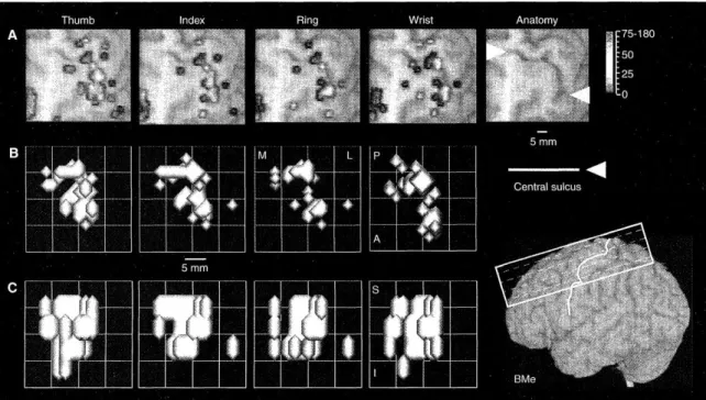
4.1 Somatotopy ... 29
4.2 Depth Structures ... 32
4.3 Visual Responses in M1 ... 34
4.4 Imagery in M1 ... 36
5 Methods ... 39
5.1 Participants ... 39
5.2 Paradigm ... 39
5.3 Image acquisition ... 40
5.4 Imaging Data Analysis ... 41
5.4.1 Preprocessing ... 41
5.4.2 Co-registration ... 43
5.4.3 Segmentation ... 43
5.4.4 Statistical parametric maps ... 44
5.4.5 Cortical grid sampling... 45
5.4.6 Veins ... 46
5.4.7 Types of data and measures ... 47
5.4.8 Statistical Analysis ... 49
6 Results ... 51
6.1 Somatotopy ... 51
6.1.1 Grids Specificity ... 51
6.1.2 Somatotopy between layers ... 55
6.1.3 Correlation between finger activity maps ... 60
6.2 Depth Structures ... 62
6.2.1 Layer connections ... 62
6.2.2 Directionality Preference of Functional Connectivity ... 64
6.3 Imagery in M1 ... 65
6.4 Visual activity in M1... 67
xiii
7 Discussion ... 73
7.1 Somatotopy ... 73
7.2 Depth Structures ... 74
7.3 Non-motor tasks ... 75
7.4 Limitations and Future Work ... 76
8 Conclusion ... 77
References ... 79
xv
List of Figures
Figure 2.1 - Subdivision of the brain structures ...3
Figure 2.2 - Representation of brain anatomic structure – main divisions ...4
Figure 2.3 -Coronal section showing the distribution of the grey and white matter in the brain ...5
Figure 2.4 - Left lateral and medial views of the cerebral hemisphere showing the landmarks used to divide the cortex into its main lobes...6
Figure 2.5 - The basic six-layered structure of neocortex ...8
Figure 2.6 - Lateral Brodmann’s areas ... 10
Figure 2.7 – A somatotopic map of the human precentral gyrus ... 11
Figure 2.8 - Main vessels of the brain ... 11
Figure 3.1 - Similarities between spinning proton and spinning magnet ... 13
Figure 3.2 – Magnetic fields cause the alignment of nuclei that have the NMR property ... 14
Figure 3.3 – Tipping over the net magnetization with excitation by radiofrequency pulse ... 15
Figure 3.4 – Free Induction Decay after a 90o RF pulse ... 17
Figure 3.5 – Image space and k-space ... 19
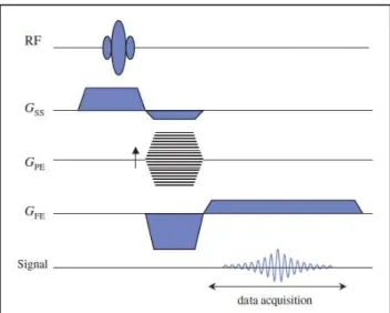
Figure 3.6 - Basic gradient echo sequence ... 20
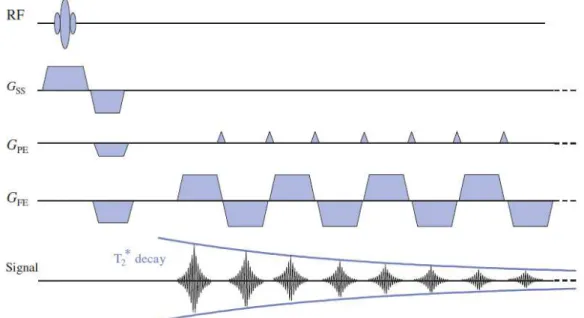
Figure 3.7 – Blipped GRE-EPI sequence ... 21
Figure 3.8 – An overview of the physiological changes leading to fMRI data ... 23
Figure 3.9 – Illustration of BOLD fMRI time series in active voxel ... 24
Figure 3.10 –Characteristics of the HRF ... 26
Figure 3.11 –Assumed fixed-shape of hemodynamic response for different experimental designs .... 27
Figure 4.1 - Human M1 homunculus ... 29
Figure 4.2 - Organization of motor cortex of a normal macaque monkey. ... 30
Figure 4.3 - Movement representation overlap ... 30
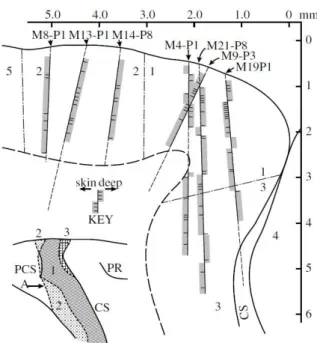
Figure 4.4 - Reconstruction of some electrode penetrations ... 32
Figure 4.5 – Cortical areas related to the mirror system ... 35
Figure 4.6 – Illustration of M1 activity during fingers motor imagery and movement execution. ... 37
Figure 5.1 - Experimental design used for all the different tasks ... 40
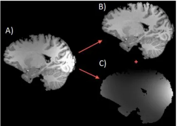
Figure 5.2- Intensity differences before and after IIC ... 43
Figure 5.3– Three dimensional activity map (FDR corrected) of middle finger during motor task for lower resolution scan ... 44
Figure 5.4 – ROI selected from the three dimensional activity map presented in Figure 5.3... 45
Figure 5.5 – Illustration representing the cortical mapping approach exemplary in subject S2 ... 46
Figure 5.6- Veins detection. ... 47
Figure 5.7 –Cortical grid’s info ... 48
Figure 5.8- Illustration of finger specific time courses selection according with the paradigm and baseline data points ... 49
Figure 5.9– Scheme of the dimensions used for time course correlation ... 49
Figure 6.1– Differential activity maps of thumb finger grid in single subject [S9] ... 52
Figure 6.2 – Direct activity maps of thumb finger grid in single subject [S9]. ... 52
Figure 6.3 – Number of active pixels averages for different finger maps in FG1. ... 53
Figure 6.4 - Percent signal change peak averages for different finger maps in both finger grids ... 54
xvi
Figure 6.6 – Average BOLD response of all subjects for two finger maps in FG3 ... 55
Figure 6.7 – Distribution of the pixels for the ME ... 56
Figure 6.8 – Number of active pixels average in the three cortical layers ... 57
Figure 6.9 –Illustrative example of the number of active pixels decrease with depth... 57
Figure 6.10 - Distribution of the active pixels for the ME ... 58
Figure 6.11 –Average BOLD response of all subjects of thumb in FG1 for the three cortical layers ... 59
Figure 6.12 –Average BOLD response of all subjects of middle finger in FG3 for the three cortical layers. ... 59
Figure 6.13 – Peak of BOLD response average for the three different layers ... 60
Figure 6.14 – Correlation indexes averages between the different finger maps of activity. ... 61
Figure 6.15 – Correlation indexes average between adjacent finger activity maps in FG1 ... 61
Figure 6.16 - Correlation indexes average of the t-maps for different pairs of layers ... 63
Figure 6.17 - Correlation values averages between the average BOLD responses of different pairs of layers ... 63
Figure 6.18 - Correlation values averages between different layer’s mean time course signals ... 64
Figure 6.19 –Correlation indexes averages between pixel’s signals for different dimensions ... 65
Figure 6.20 – Direct activity maps of two tasks (motor imagery and motor execution-ME) for the middle finger grid of a single subject [S3] ... 66
Figure 6.21 – Differential activity maps of two tasks (motor imagery and motor execution-ME) for the thumb finger grid (FG1) of a single subject [S9] ... 67
Figure 6.22 – Direct activity maps of two tasks (movement observation - MO and motor execution-ME) for the thumb grid (FG1) of a single subject [S6] ... 68
Figure 6.23 – Direct activity maps of two tasks (movement observation - MO and motor execution-ME) for the middle finger grid (FG3) of a single subject [S6] ... 68
Figure 6.24 – Average correlation values between the matching activity maps of different task pairs ... 70
xvii
List of Tables
xix
Abbreviations and Acronyms
ANOVA BOLD CBF CBV CMRO2 CSF E EEG EPI EV FDR FFT FG1 FG3 FID FM1 FM2 FM3 fMRI FOV FSTC GFE GPE GSS GRE GLM GM HRF IIC IV M1 ME MEG MP-RAGE MO MRI MT NMR OD PD PMC
Analysis of Variance
Blood Oxygen Level Dependent Cerebral Blood Flow
Cerebral Blood Volume
Cerebral Metabolic Rate of Oxygen Cerebrospinal Fluid
Local Oxygen Extraction Fraction Electro-Encephalography Echo-Planar Imaging
Extra-vascular BOLD component False Discovery Rate
Fast Fourier Transform Thumb Finger Grid Middle Finger Grid Free Induction Decay Thumb Activity Map Index Finger Activity Map Middle Finger Activity Map Functional Magnetic Ressonance Field of View
Finger Specific Time Course Frequency Encoding Gradient Phase Encoding Gradient Slice Selection Gradient Gradient Echo
General Linear Model Grey Matter
Hemodynamic Response Function Intensity Inhomogenity Correction Intra-Vascular BOLD component Primary Motor Cortex
Motor Execution
Magneto- Encephalography
Magnetization Prepared Rapid Gradient Echo Movement Observation
Magnetic Ressonance Imaging Middle Temple Visual Area Nuclear Magnetic Ressonance Ocular Dominance
xx rER RF ROI SE SMA SNR STS T1 T2 T2* TE TMS TR V1 V2 V4 V5 WM µ ƴ B0 J M0 ν0
Rough Endoplasmatic Reticullum Radiofrequency
Region of Interest Spin Echo
Supplementary Motor Area Signal to Noise Ratio Superior Temporal Sulcus Longitudinal Relaxation Time
Apparent Transverse Relaxation Time Transverse Relaxation Time
Time to Echo
Trans-cranial Magnetic Stimulation Time to Repetition
Primary Visual Cortex Prestriate Cortex
Visual area located in the extrastriate cortex Visual area MT
White Matter
1
1
Introduction
1.1
Project Presentation
Due to a powerful tool - the advent of functional magnetic resonance imaging (fMRI), the knowledge related with the human brain has been exponentially increased. Most notably, novel techniques using ultra-high fields allow astounding data quality, with resolutions capable of imaging different cortical laminas; bringing a brighter future not only for neuroscience, but also to other science fields like medicine.
Allying this and other techniques, cognitive neuroscience has accomplished a new level of knowledge, especially regarding the functioning of the motor system.
The capacity to perform a complex sequence of movements, linking all the basic actions is the main component of voluntary motor behaviour. To process such detailed information, the brain uses different regions, for instance primary motor cortex (M1). From a classical view, M1 is responsible for the final cortical output of movement commands, while recent studies point to more complex roles for M1 in orchestrating motor-related information.
Several conflicting theories and findings have shown different features for imagery and visual activity in M1 or even for somatotopy (the idea that body representations follow a specific and ordered pattern) in the primary motor cortex. Additionally no studies have been performed in humans to analyze the existence of cortical columns structures in M1.
Therefore, the purpose of this project is to study the primary motor cortex in a laminar level using ultra-high fMRI. The complex functioning of M1 was studied in three different tasks: movement, observation and imagery of fingers tapping. Furthermore, different cortical laminas of human M1 were analyzed for the first time: providing a better understanding of somatotopy and cortical connections in depth. Accordingly, this study aims to answer to the following questions:
- Is there a somatotopic or distributed representation for fingers in M1? - Are there any depth structures in human M1?
- Is M1 activated by action observation? - Is M1 activated by motor imagery?
1.2
Structure of the thesis
The present thesis is divided in seven chapters, involving a theoretical background for a better understanding of the current work; a description of the images acquisition process and the data
analysis, as well as a result’s discussion and final conclusions.
2 the third chapter, as well as the functioning of Functional Magnetic Resonance Imaging (fMRI). The same chapter also includes a report about ultra-high field MRI.
In order to summarize all the scientific information related with this project, Chapter 4 consists in a literature review.
The methodology used for this study is described in Chapter 5. It includes the methods applied for the acquisition and processing of the images, as well as the ones used to analyze the results (measures and statistics). The obtained results are presented in Chapter 6.
3
2
Neuroanatomy
The human brain has fascinated and baffled people throughout the centuries, from nowadays scientists to our prehistoric ancestors. During the last decades, researchers have developed novel techniques to improve the knowledge about human brain functioning and its structures.
Even though, the attempt to understand the functional organization of the brain has proven to be a daunting challenge. Mostly, due the slow development of the experimental tools to measure and map brain activity, because its structures are minute and highly complex.
Since this work focuses on the brain’s cortical motor network the following section presents some general considerations about this organ.
2.1
Brain Structure
As the maestro of the body, with 100 billion nerve cells, brain has a complex anatomy and a tiered structure.
The normal adult human brain in average weights 1.4 Kg and which corresponds to only 2% of the body weight. Yet the energy-consuming processes account for approximately 25% of total body glucose utilization(Carter et al., 2009a; Squire, 2013).
From a gross point of view, this organ can be subdivided into the cerebrum, the brain stem and the cerebellum. The scheme bellow (Figure 2.1 - Subdivision of the brain structures) shows a detailed division and in Figure 2.2 there is an anatomical representation.
Brain (Encephalon)
Cerebrum (forebrain)
Telencephalon
- Cerebral cortex - Subcortical white
matter -Commisures - Basal ganglia
Diencephalon
- Thalamus - Hypothalamus
- Epithalamus - Subthalamus
Cerebellum - Cerebellar cortex - Cerebellar nuclei
Brain stem
- Midbrain (mesencephalon)
- Pons - Medulla oblongata
4 The most complex functions occur in the cerebrum(Carter et al., 2009b).
For instance, the hypothalamus has many vital roles such as conscious behavior, emotions and instincts, and automatic control of body processes. The thalamus screens and preprocesses all the flux of sensory information and sends it on to the cerebral cortex.
Finally, the cortex is responsible for conscious, discriminative aspects of sensation; and cognitive activity, including language, reasoning, and many aspects of learning and memory.
On other hand, the brain stem and cerebellum main functions are essential to complement the brain functioning.
For example, subconscious or autonomic regulation mechanisms are controlled by the brain stem. In medulla stand the centers for respiratory, cardiac and vasomotor monitoring and command. Even the pons is involved in learning and remembering motor skills.
Finally, body movement coordination (like balance and posture) is ordered by cerebellum(Carter et al., 2009a; Snell, 2010).
Most of mammal’s cortical brain networks have been described, although structural connection data
for the human brain is largely missing (Crick and Jones, 1993).
Figure 2.2 - Representation of brain anatomic structure – main divisions (Sch n e et al., 2010)
Note that: in the Figure 2.2 are two structures, that haven’t been yet referred - corpus callosum and pituitary.
The largest commissure1 of the brain, corpus callosum, contains more than 200 million nerve fibers that link the cerebral hemispheres.
Pituitary is an endocrine gland, which is regulated by hypothalamus. It thus controls a variety of bodily functions, such as growth, heart rate, muscle contraction, sexual behavior among others (Carter et al., 2009a; Snell, 2010).
5
2.2
Cerebral Hemispheres
The cerebrum constitutes more than three-quarters of the brain’s total volume and is divided in two cerebral hemispheres (telencephalon), which include the cerebral cortex, the cerebral white matter (comissures and subcortical white matter) and a complex of deep gray matter masses, the basal ganglia.
Basically, the cerebrum has two types of tissue – white and grey matter (Figure 2.3).
The gray matter consists of neuronal cells bodies and gial cells1, axons2, dendrites3 and synapses4. While, the white matter (WM) contains axons and theirs associated gial cells. Many axons are
myelinated5, allowing rapid nerve impulse conduction and giving WM its pale appearance (Snell, 2010; Squire, 2013).
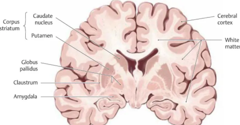
Figure 2.3 -Coronal section showing the distribution of the grey and white matter in the brain (Sch n e et al., 2010)
According to Figure 2.3, the structures of the telencephalon compound by grey matter are: - Cerebral cortex;
- Basal ganglia: the caudate nucleus and putamen (collectively called the corpus striatum) and globus pallidus;
- Other grey matter nuclei that are not included among the basal ganglia: claustrum and amygdale (often considered a transitional form between the two types of gray matter – cortex and basal ganglia) ch n e et al., 2010).
The surfaces of the cerebral hemispheres contain many gyri6, sulci and fissures, in a way that more
than 50% of the cortex’s area approximately 0.8 m2
) is hidden within the grooves7.
Therefore, their presence, in a pattern that is relatively constant from brain to brain, allows to separate different cortical areas: frontal, parietal, occipital and temporal, insular and limbic lobes (Figure 2.4). In some naming systems, the limbic and insular lobes are distinguished as separate from other lobes (Krieg, 1946; Carter et al., 00 a ch n e et al., 2010; Snell, 2010).
1- These cells appear to play important roles in supporting and protecting neurons, like myelin formation or guidance of developing neurons.
2- Specialized structure that conducts electrical signals from the initial segment (near the cell body) to the synaptic terminals.
3- Extensions of neurons that stretch out from the cell body; they receive incoming synaptic information and thus, together with the cell body, constitute the receptive pole of the neuron.
4- Interneuronal complex responsible for the communication between neurons.
5- Covered with myelin (multiple concentric layers of lipid-rich membrane which functions as an insulator).
6- Rounded bulges of the cortex;
6
The cerebral hemispheres are separated by the main and deepest groove- the longitudinal fissure.
The central sulcus, also known as the fissure of Rolando, arises about the middle of the hemisphere and separates the frontal lobe from the parietal lobe.
Note that, the insular lobe lies deep within the lateral sulcus.
7
2.3
Cerebral cortex
The cerebral cortex is the outer layer of the cerebrum, constituting about 40% of the brain by weight and contains an average of 16 billion neurons (Herculano-Houzel, 2009).
There are two types of cortices:
- Allocortex (three layered cortex, mostly found in the limbic system cortex)
- Neocortex (more frequently found in most of the cerebral hemisphere and contains six layers)
There is also mesocortex (a form of neocortex), which makes the transition between the allocortex and isocortex. It contains three to six layers and it includes such regions as the cingulate gyrus and the insula.
The allocortex and mesocortex incorporate the limbic lobe, while the neocortex consists of the cortex of all the cerebral lobes, excluding the allocortex (Snell, 2010; Strominger et al., 2012).
2.3.1
Organization of the neocortex
As already referred, the neocortex consists of six layers parallel to the cortical surface, each of which is usually named after its predominant cell type.
Main Neurons of the Neocortex
There are four main types of cells arrange in this layered structure: pyramidal, stellate, granulate and spindle (fusiform) cells Brodal, 0 0 conomo and riarhou, 00 ch n e et al., 2010; Snell, 2010).
Pyramidal cells usually contain well-developed Nissl bodies1. They have a triangular shape, being elongated in the vertical direction. Their size may vary substantially, so, there are: small and large pyramidal neurons.
The small pyramidal neuron is a cell with a long axon that usually ends within the cortex, either as: - Association fiber (axon links two different cortical areas within the same hemisphere); - Commissural fiber (axon passes in the corpus callosum and connects areas in opposite hemisphere but in a cortical area of similar function)
These types of pyramidal cells have the property to project neurons whose axons end within the cortex. On other hand, the large pyramidal neuron is a cell with a very long axon that projects outside the cortex, even for distant structures.
The stellate neuron has a short axon to process local information. They have inhibitory (aspiny neurons) and excitatory (spiny stellate cells) properties. Stellate cells exhibit a variety of shapes, such as: double bouquet cells, tuft cells, chandelier cells and basket cells.
Stellate and pyramidal cells can also be distinguished by the arrangement of their dendrites. Pyramidal cells have an apical dendrite2 and basilar dendrites3. While, the stellate cells (star shaped) have dendrites exending in all directions.
1- Large clumps of rough endoplasmic reticulum (rER) in the cytoplasm of neurons, also called tigroid granules 2- Dendrite reaching from the upper end toward the cortical surface
8 Granule cells are round or polygonal, often triangular (similar to the stellate cell morphology). This is the generic term for a small neuron; in fact it has a very short cytoplasm, because the nucleus occupies most of the cell.
Fusiform cells are long and spindle shaped with an apical dendrite together with numerous dendrites radiating from the cell body. These cells combine the features of both stellate and pyramidal cells
Brodal, 0 0 conomo and riarhou, 00 ch n e et al., 2010; Snell, 2010).
Layers of the Neocortex
The neurons of the neocortex are arranged in six well-defined layers (Figure 2.5), or laminae, known generally from the outside inward (from the surface of the cortex to the WM) as the molecular, external granular, external pyramidal, internal granular, internal pyramidal and multiform layers
matter Brodal, 0 0 conomo and riarhou, 00 ch n e et al., 2010; Snell, 2010; Strominger et al., 2012) .
The outermost cortical layer - the molecular layer (I) - is abundant in fibers, that come from within the cortex or from the thalamus. The neurons in this layer are few in number, apart from that, layer I also contains apical dendrites of pyramidal cells in the deeper layers.
Figure 2.5 - The basic six-layered structure of neocortex - The three columns show perpendicular sections to the cortical surface to different staining1 methods. Left: Appearance in Golgi-stain2. Middle: A thionine-stained section3. Right:
Appearance after myelin staining4. (Brodal, 2010)
1- Auxiliary technique used in to highlight contrast in the microscopic image
9 4- Another kind of staining, in which the major pattern of the myelinated axons is clear, where perpendicular bundles of fibers are entering the cortex, and the ones horizontal are interconnecting close regions of the cortex.
The second layer is the external granular layer (II). It is a fairly dense layer comprised of numerous small granule cells. The name of this layer is misleading because it is largely populated by small pyramidal neurons.
Right beneath layer II is the pyramidal cell layer (III). It is thick and pyramidally shaped cells prevail (they are larger in size, not in number), but it also contains another kinds of cell types.
The size of neurons increase with depth, which means that the ones located deeper in this layer are typically larger than those located more superficially.
Layer IV, the internal granular layer, usually a thin layer, is made up primarily of granule cells, its densely packed somata is similar to the one in layer II.
The internal pyramidal layer (V) mainly consists of pyramidal cells, these are typically larger than those in layer II.
The last layer (VI) is called the polymorphic/fusiform/multiform layer, due to its heterogeneous somata, main of which belongs to spindle-shaped cell bodies. This layer forms the deep limit of the cortex, whose axons go through the adjacent WM Brodal, 0 0 conomo and riarhou, 00
ch n e et al., 2010; Snell, 2010; Strominger et al., 2012).
The layers diverge regarding to their connections - afferent and efferent.
Generally, layers II and IV are receiving, when in fact layers III and V are essentially efferent. The afferents connections extend from the thalamus to lamina V, whereas layer V is the starting point to subcortical tracts to the cord, brain stem and basal ganglia. Layers II and III receive and send out their axons primarily to other areas of the cortex (association and commissural fibers). The layer VI is also largely efferent and sends many axons to the thalamus (Brodal, 2010).
2.3.2
Functional areas
The details of layer’s functional organization vary throughout the cortex. o, the cortex has been divided in various ways, the most used demarcation system is that of Brodmann (1909), who took advantage of Nissl-stained preparations to visualize the distribution of the neurons in different layers of neocortex (cytoarchitectonics) and number the functional areas of neocortex. More than 40 areas are distinguished on the lateral (Figure 2.6) and medial surfaces of the brain ch n e et al., 2010; Strominger et al., 2012).
Cortical Microstructure: Columns
While morphological considerations separate the cerebral cortex into horizontal layers, functional considerations guide to its division into distinct units or modules.
At a microstructural level, the cortical neurons appear to be organized into small modules formed by cylinders or columnsof tissue extending perpendicular to the surface of the cortex. These modules of tissue contain neurons whose salient physiological properties are identical.
10
Figure 2.6 - Lateral Brodmann’s areas (Carter et al., 2009)
2.4
Primary motor cortex (M1)
Brodmann area 4 is the primary motor cortex, located on the anterior wall of the central sulcus.
Not all cortical regions have the same laminar organization. For example, the precentral gyrus, also known as M1, has almost no internal granule layer (layer IV) and thus is called agranular cortex. The lack of prominence of layer IV can be understood because of its connections with the thalamus. Layer IV is where the sensory information arrives from the thalamus. The motor cortex is principally an output area of the neocortex, therefore slightly receives sensory information directly from the thalamus (Kandel et al., 2000).
There are also changes within cortical regions related to layer’s constitution. For instance, exceptional large pyramidal neurons, known as Betz cells, are restricted to cortical lamina V of M1. These cells are in charge of voluntary movements on the opposite side of the body, with the impulses traveling over their axons.
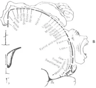
M1 has a somatotopic organization, which means that M1 has specific regions in the cortex to control the movement of different parts of the body. Homonculus is the cartoon that magnifies some parts of the body with respect to cortical territory, by distorting the size of body parts relative to their normal proportions (Penfield and Boldrey, 1937; Squire, 2013).
11
2.5
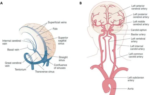
Blood vessels of the head
As expected, the brain and all our body are critically dependent on an uninterrupted supply of oxygenated blood. Nearly 20% of the blood body circulates in the brain, which represents 2% of the body weight. Brain vessels (Figure 2.8) provide the means for this uninterrupted blood supply (Snell, 2010).
There are variations among individuals in the vessel’s size, positioning and even in their number.
1-Venous sinuses are venous channels of the dura mater one of the three brain’s connective tissue layers)
A B
Figure 2.7 – A somatotopic map of the human precentral gyrus (M1): showing the specific regions in this cortex to control the movement of different parts of the body(Squire, 2013)
12 The blood transports oxygen, nutrients, and other necessary substances to keep the brain tissues working properly. The arteries carry the oxygenated blood with all the nutrients and the veins carry the deoxygenated blood.
13
3
Magnetic Resonance Imaging (MRI)
Magnetic resonance imaging has become an important tool for neuroscientists, because it can be used non-invasively to obtain high-quality images of the brain or other organs/structures of the body without radiation, as is necessary for X-ray imaging. The technology behind this technique is complex, but it is essential to understand in order to entirely appreciate MR images of the brain.
3.1
Basic Principles
As the name suggests, magnetic resonance imaging uses the magnetic properties of tissue to produce an image.
3.1.1
Nuclear Magnetic Resonance and Equilibrium Magnetization
All magnetic resonance imaging relies on a few physical principles that were discovered by Rabi, Bloch, Purcell and others (Geva, 2006). They performed the first successful experiments, demonstrating the phenomenon of NMR – Nuclear Magnetic Resonance. Certain nuclei have an intrinsic magnetic moment and, when placed in a magnetic field, they rotate with a frequency proportional to the field (Buxton, 2009).
Consider a single hydrogen atom. In regular conditions, thermal energy lets the proton to spin about its axis (Figure 3.1A); his precession motion has two effects: first its spin creates superficial electrical current, which origins a magnetic source. The strength of this magnetic source per unit of magnetic field is the magnetic moment (µ). Second, because the proton has an odd atomic mass number, its spins results in an angular momentum (J). Due to the right-hand rule, both µ and J are vectors pointing in the same direction (Huettel et al., 2009).
Basically, as the nuclei spins, the changing magnetic field produces a magnetic moment and the moving mass results in angular momentum.
For a nucleus to be useful for MRI, it must possess nuclear magnetic resonance properties – have both a magnetic moment and an angular momentum.
Only a few atoms have the required properties - 1H, 13C, 19F, 23
Na and 31P; the hydrogen is the most used, due to its abundance in the living organisms, for example an average person contains approximately 5x1027 hydrogen protons (Huettel et al., 2009).
These hydrogen protons can be thought of as little magnets (Figure 3.1): they spin about an axis and their spinning positive charge induces a minuscule magnetic field. In absence of an external magnetic field (B0), due to different axis of precession, the magnetic fields of individual protons orient in random directions and the equilibrium magnetization1–M0– is null, because x, y and z components
cancel each other (Figure 3.2A) (Carter and Shieh, 2010).
1-The net magnetization is the sum of all the magnetic moments of each of the H nuclei within a system
14 Now consider one of these spins located in an external magnetic field (B0). This external field exerts a torque on the proton that would tend to align the proton spin with B0.
However, because the nucleus also has angular momentum, it instead gains a gyroscopic motion known as precession (Figure 3.2C). This movement is analogous to a spinning top in a gravitational field. In this case, the spin precesses around an axis parallel to the main magnetic field, maintaining a constant angle.
The precession frequency - Larmor frequency, ν0, is the resonant frequency of a spin within a
magnetic field and is proportional to the strength of the applied field (B0):
Equation 3.1
Where:
- is the gyromagnetic ratio (constant for a given type of nucleus) and it corresponds to the ratio between the charge and mass of a spin. For the hydrogen nucleus it corresponds to 42.58 MHz/T (Buxton, 2009).
There are two states for precessing spins (Figure 3.2B): one low energy state (parallel to the magnetic field, spin = -½) and one high energy state (anti-parallel to the magnetic field, spin = ½). Thus, more energy is required for the anti-parallel direction, which translates into a (small) preference for the parallel alignment.
As a result, when a system of these nuclei, for example the human body, is placed in a magnetic field (B0) the net magnetization is no longer null, because in the equilibrium state there are slightly more
spins aligned in the parallel direction (Figure 3.2B). This small difference creates a weak magnetization in the same direction of B0. ince the protons involved don’t spin in phase, the
resultant vector, M0, doesn’t show any transversal (xy axis) component (Carter and Shieh, 2010).
Even though this weak magnetization is not directly observable, in certain conditions it can be measured and it is the basis of all observable NMR signals.
15
3.1.2
Excitation and Detection
The resonance phenomenon corresponds to an exchange of energy between two systems at a specific frequency. Hence, in order to measure M0, a radiofrequency (RF) pulse oscillating at Larmor
frequency is created producing a magnetic field B1 perpendicular to B0. This RF pulse is generated by
a transmitter coil.
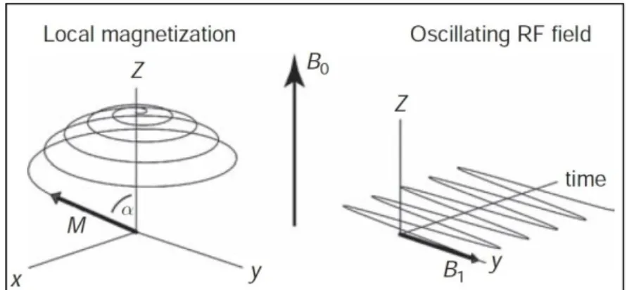
The new field, B1, is several orders of magnitude smaller than B0. Nevertheless, this causes
disturbances among the parallel aligned protons, because some of them, gradually, will absorb the electromagnetic energy and jump to the high-energy state, process known as excitation. The effect is that with each precessional rotation M0 tips farther away from B0, tracing out a widening spiral
(Figure 3.3).
These RF pulses are regularly characterized by the flip angle (α) they make. The flip angle can be controlled by the strength and duration of the RF pulse. The new magnetization (tipped M0) is
represented by M (Figure 3.3).
Basically, during excitation, longitudinal magnetization decreases and a transverse magnetization develops (excluding for a
180° flip angle).
Longitudinal magnetization is due to a difference in the number of spins in parallel and anti-parallel state. Transverse magnetization is due to spins getting more or
less phase coherence
(Imaios, 2013).
A 90º degree excitation
pulse results in an equal numbers of spins in low and high energy states. This can be seen as the rotation of the net magnetization from the longitudinal direction (z axis) into the transverse plane (xy axis). In this case, the application of a 90º RF pulse also brings the spins to complete phase coherence (Imaios, 2013).
When the net magnetization is along the longitudinal axis, the individual spins precession cannot be measured in detector coils. But when the net magnetization acquires a transverse compound via excitation, its precession around the main magnetic can generate an oscillating electric current in reception coils with the scanner (applying the Faraday’s law of induction) (Huettel et al., 2009; McRobbie, 2007).
Note that typically, the coil is used as both a transmitter and a receiver. During the transmit phase of the experiment, an oscillating current is applied to the coil for a brief time. During the receive phase of the experiment, the coil is connected to a detector circuit that senses the small oscillating currents in the coil.
16
3.1.3
Relaxation times
The MR signal detected through receiver coils does not remain stable forever. After a time, the RF field is turned off and the spins will eventually return into the equilibrium state in a process known as relaxation.
The relaxation mechanisms depend on spins interaction with the surroundings and behaves differently in different tissues. The relaxation of excited spins combines two different mechanisms: longitudinal relaxation and transverse relaxation (Imaios, 2013).
Longitudinal relaxation
Longitudinal relaxation or spin-lattice relaxation refers to a phenomenon of energy exchange between the spin system and the surrounding environment. As spins pass from a high energy state to a low energy state, RF energy is released back to re-establish thermal equilibrium.
These energy transferences give rise to the recovery of the longitudinal magnetization: an increasing in the longitudinal component of the flipped net magnetization vector from M to M0(Imaios, 2013).
The recovery rate is characterized by the tissue-specific time constant T1, which corresponds to the
time taken for the magnetization to recover to 63% of its equilibrium value(McRobbie, 2007). According to the Bloch equations, the amount of longitudinal magnetization, Mz, present at time t
following an RF pulse is given by:
Equation 3.2
Transverse relaxation
Transverse relaxation or spin-spin relaxation results from spins losing their phase coherence. As spins collectively move, their magnetic fields interact (spin-spin interaction), vaguely changing their precession rate. These interactions incite a cumulative loss in phase coherence producing transverse magnetization decay.
The transverse relaxation is characterized by a time constant represented as T2 - the time taken for the transverse magnetization to drop to 37% of its initial size (Imaios, 2013).
According to the Bloch equations, the amount of longitudinal magnetization, Mxy, present at time t
following an RF pulse is given by:
Equation 3.3
Equation 3.4
Where Mx is the transverse magnetization in the x axis and My is the transverse magnetization in the
y axis.
17 The decay of transverse magnetization arises from magnetic field inhomogeneities. These inhomogeneities may be intrinsic or extrinsic, i.e. internal to the proton system or external in the scanner. Note that, only the intrinsic inhomogeneities contribute to T2 (McRobbie, 2007).
An extrinsic source of differential spin effects is the external magnetic field, which is usually inhomogeneous. Each spin precesses at a frequency proportional to its local field strength; as a result, spatial variations in field strength provoke spatial differences in precession frequencies. This additional decay caused by extrinsic inhomogeneities has been called T2’decay (Buxton, 2009; Huettel et al., 2009).
The combined effects of cumulative phase differences (intrinsic inhomogeneities) and local magnetic field inhomogeneities lead to signal loss known as T2* decay, characterized by the time constant T2*:
Equation 3.5
During relaxation, protons re-radiate the absorbed energy: this will induce a current in a nearby coil, creating a measurable signal that is proportional to the magnitude of the transverse magnetization. This detected signal is called free induction decay (FID) and is illustrated in Figure 3.4.
This signal decays away exponentially and the time constant for this decay is:
- T2 in a perfectly homogeneous magnetic field;
- T2
*
in an inhomogeneous magnetic field.
-3.2
Image Acquisition
3.2.1
Signal Detection: Spatial Localization
In the theory described above the magnetic resonance signal is introduced as a global signal from a sample. In order to create MR images signal must be divided into components with different frequency parameters in a method known as spatially encoding; so it can be detected from different spatial locations.
Spatial encoding relies on successively applying magnetic field gradients. To resolve spatial information in three dimensions (x, y and z), we need at least three gradient fields. Therefore in an MR scanner, there are three gradient coils in addition to the RF coils and the coils of the magnet itself. Each gradient coil produces a magnetic field that varies linearly along a particular axis (Buxton, 2009).
Spatial localization is made in three steps: slice selection, phase encoding and frequency encoding; each step is related with one gradient: slice selection gradient (GSS), phase encoding gradient (GPE) and frequency-encoding gradient (GFE). The different gradients have identical properties but are applied at distinct moments (Imaios, 2013).
18 In the first step (slice selection), a gradient (GSS) is turned on along the slice selection axis (z, perpendicular to the desired slice), consequently the precession frequency of the protons varies linearly along the z direction. An RF wave is simultaneously applied with a bandwidth that contains the range of precession frequencies in the desired slice plane. This causes a shift in the magnetization of only the protons on this plane. As no protons located outside the slice plane are excited, they will not emit a signal.(Buxton, 2009; Imaios, 2013)
The phase encoding consists of applying a magnetic field gradient (GPE) in the vertical direction (y axis) of the slice selected in the first step. While it is applied, it modifies the spin resonance frequencies, inducing dephasing, which persists after the gradient is interrupted (Imaios, 2013). After this step, all the protons precess in the same frequency but each local precessing magnetization is marked with a phase offset proportional to its y-position.
During frequency encoding, a magnetic field gradient (GFE) is applied in the horizontal direction (x axis) of the slice selected in the first step. This gradient modifies the spin resonance frequencies along the horizontal direction. It thus creates proton columns, which all have an identical Larmor frequency. This gradient is applied during the data acquisition period.
The repeated combination of the three gradients allows the formation of a 3D image.
Note that, the imaging coordinate system can have any orientation relative to the magnetic field, even though both the direction of B0 and the axis perpendicular to the image plane are usually referred to as the z-axis. (Buxton, 2009)
Any spatial localization method has resolution limits, in this case these limits can be represented in terms of a volume resolution element (voxel) with dimensions (Δx, Δy, Δz) (Buxton, 2009).
3.2.2
Image Formation
The collected data from the same slice - a mix of RF waves with different amplitudes, frequencies and phases, containing spatial information - is stored in the k-space (Fourier space) and requires a 2D inverse Fourier Transform to form an image of the slice plane, as illustrated in Figure 3.5.
Fourier transform is a mathematical procedure that allows the transformation of a time domain signal into a frequency domain signal (a spatial frequency in the case of fMRI) (Imaios, 2013).
The central portion of k-space describes the low-spatial-frequency components, which in image space is traduced in the lowest intensity change. On other hand, the outer edges describe the high frequencies, which determine image brightness, but no detail (Buxton, 2009; McRobbie, 2007).
There are several ways to fill the k-space, like linear filling, centric or spiral. The easiest way to fill the k-space is to use a line-by-line rectilinear trajectory. One line of k-space is fully acquired at each excitation, containing low and high-horizontal-spatial-frequency information (contrast and resolution in the horizontal direction). Between each repetition, there is a change in phase-encoding-gradient strength, corresponding to a change in ky-coordinate.
19
Figure 3.5 – Image space (left) and k-space (right): Any MR image can be represented as a matrix of intensities on the image space or as a matrix of spatial frequencies on the k-space (Buxton, 2009)
3D imaging
The methods described so far, using a slice selection to define each single slice, are all intrinsically two-dimensional methods, but true three-dimensional imaging also can be performed.
The principle is simply to excite a complete volume, rather than one thin slice and to apply a second phase-encode axis in the third dimension (z axis).
This translates in particularities in k-space, now a 3D space: in order to fill this new space the number of repetitions increases in a factor equal to the number of « slices» (partitions) in the third dimension. Obviously, the image reconstruction is performed by an inverse 3D Fourier Transform (Imaios, 2013).
The advantages of 3D acquisitions consist in getting thinner and more slices with better profiles, and better signal to noise ratio (SNR) for an equivalent slice thickness. The disadvantages are longer acquisition time and possible artifacts1 (McRobbie, 2007).
While the majority of MRI data is multi slice, the anatomical data acquired for this project were 3D acquisitions.
3.2.3
MR pulse Sequences
The arrangement of radiofrequency pulses and magnetic gradients used to collect a given type of MR image is known as a pulse sequence. The basic format of a pulse sequence diagram consists of a series of horizontal lines, each representing how a different component of the scanner changes over time (Huettel et al., 2009).
The essential components for any imaging sequence are: an RF excitation pulse; gradients for spatial encoding (2D or 3D); signal reading. When performing an image acquisition, the user must choose the sequence parameters. One essential parameter is echo time (TE) - the time between the 90° RF pulse and MR signal sampling, corresponding to maximum of echo. The other is the repetition time (TR) - the time between two pulse sequences applied(Imaios, 2013).
20 There are several types of sequences; the aims are to find the best compromise between contrast, spatial resolution and speed. New pulse sequences are being created every day, but there are two main sequence families: spin echo (SE) and gradient echo (GRE) sequences.
Spin Echo
SE sequences are made up of a series of events. First, a 90° RF pulse is applied to tip the magnetization into the transverse plane. Due to field heterogeneities spins star to lose phase coherence. So, in order to compensate this dephasing effect at one-half of the echo time a 180° RF pulse is applied. With this rephasing pulse, the signal is characterized in T2 and not in T2
*
. Finally, the signal reading is performed at TE (Imaios, 2013).
Gradient Echo
GRE sequences (Figure 3.6) differ from SE sequences in regard to: the RF pulse applied, which has a variable flip angle, usually below 90° and the absence of a 180° RF rephasing pulse.
As GRE techniques use a single RF pulse and no 180° rephasing pulse, the signal obtained is thus characterized in T2* rather than in T2. In this case the gradients are used to dephase and rephase the transverse magnetization.
The gains of low-flip angle excitations and gradient echo techniques are faster acquisitions, new contrasts between tissues and a stronger MR signal in case of short TR (Imaios, 2013).
Fast Imaging
New image acquisition techniques have allowed to significantly reduce the acquisition time.
One method to do it is to collect the data corresponding to more than one phase-encoding step from each excitation. There are a number of schemes for doing this; one of them is echo planar imaging (EPI).
EPI is the fastest acquisition method in MRI, but has a limited spatial resolution. It is based on: an excitation pulse; continuous signal acquisition in the form of a gradient echo train, to acquire total or partial k-space (single shot or segmented acquisition); readout and phase-encoding gradients
21 adapted to spatial image encoding with some possible trajectories to fill k-space (constant or intermittent phase encoding gradient, spiral acquisition etc.) (Imaios, 2013).
There are several EPI possibilities, like: GRE-EPI (gradient echo EPI) and SE-EPI (spin echo EPI), among others (Edelman, 2006). In the figure below (Figure 3.7) one variance of GRE-EPI is represented.
Another fast imaging technique is MP-RAGE (magnetization prepared rapid gradient echo) a 3D-imaging sequence, which combines a periodic inversion pulse1 (to enhance the signal characteristic in T1) with a rapid GRE acquisition to produce images of high spatial resolution with good contrast between gray matter and WM (Buxton, 2009).
3.2.4
Contrast and Weights
In MR images, the contrast depends on the acquisition method used. The intensity difference of the obtained signal between the different measured tissues is called contrast. It also can refer to the physical quantity being measured (T1, T2, T2*, PD2).
Each tissue has characteristic relaxation times (T1 and T2) and different proton density. In the Table 3.1 are presented a few typical values of T1 and T2 of some brain tissues
Table 3.1 Rough values for the relaxation times at field strength of 1.5 T (Buxton, 2009)
1 – The inversion pulse corresponds to a 180° RF wave which flips longitudinal magnetization in the opposite direction. Due to longitudinal relaxation, longitudinal magnetization will increase to return to its initial value, passing through null value.
(Imaios, 2013)
2 – PD refers to proton density (the number of protons present within each voxel)
Figure 3.7 – Blipped GRE-EPI sequence: an intermittent (blipped) phase encoding gradient translates in a regular path to fill k-space, making reconstruction easier and quicker than with a constant phase encoding gradient, which produces an
22 The image weighting depends on the main parameters (TR and TE) of the applied sequence: a long TR and short TE sequence is usually called PD –weighted; a short TR and short TE sequence is generally called T1-weighted; finally, a long TR and medium long TE
1
sequence is usually called T2-weighted.
A tissue with a long T1 and T2 (like water) is dark in the T1-weighted image and bright in the T2-weighted image. Thus, a tissue with a short T1 and a long T2 (like fat) is bright in the T1-weighted image and gray in the T2-weighted image (Imaios, 2013).
Note that, like T2-weithted images, T2 *
contrast is provided by pulse sequences with long TR and medium TE values. An additional requirement is that these pulse sequence use magnetic field gradients to generate the signal echo, instead of refocusing pulses, which eliminate field inhomogeneity effects (Huettel et al., 2009).
3.2.5
Image Parameters
The images obtained by magnetic resonance are created in a bi-dimensional grid of numerous pixels in different intensities. The acquisition matrix and the field of view (FOV) characterize the image. This matrix corresponds to the number of pixels along the frequency-encoding (FE) and phase-encoding (PE) axes (Edelman, 2006). Because the imaging process collects data from a certain slice thickness, there is a volume associated with each pixel, called a voxel (from “volume element”) (Buxton, 2009).
FOV is the area that contains the object of interest, thus it defines the size of spatial encoding. The smaller the voxels are, the higher the spatial resolution will be. However, it is important to realize that a high level of spatial resolution is useless if there is insufficient SNR to support it.
We can calculate the voxel size in all three dimensions from the field of view (FOV), matrix and slice thickness (McRobbie, 2007):
3.2.6
Point Spread Function
The modification between what is measured and reality is presented by the point spread function (PSF).
Consider imaging a single, small point source, ideally, the result would be only a single pixel lit up. Instead, the point source is spread out over many pixels in the image.
An ideal, true image of a continuous distribution of magnetization would specify an intensity value for every point in the plane. However, the resulting image is a convolution of the true image with PSF (Buxton, 2009).
Researchers have developed some models to recover the original image and diminish this blur effect.
23
3.3
Functional Magnetic Resonance
One of the remarkable developments on MRI work - functional MRI (fMRI) - is an indirect method of imaging brain activity at high temporal resolution. The principle relies on detecting changes in the metabolic state of the brain with MR signal. ince early 0’s, this technique has grown explosively to become an indispensable tool in neuroscience research (Ogawa et al., 1990).
Note that, the term functional MRI or fMRI has become synonymous with brain activation imaging using the BOLD effect.
3.3.1
Physiological basis of brain activation and BOLD effect
In a typical fMRI experiment the goal is to map patterns of neuronal activation in the subject's brain while the same performs specific tasks. However, fMRI does not measure the neuronal activity itself. In its place, it creates images of physiological changes that are correlated with neuronal activity.
Neuronal activity provokes an increase in oxygen consumption and an even higher increase in cerebral blood flow (CBF). In addition, the blood volume (CBV), the cerebral metabolic rate of oxygen (CMRO2) and blood velocity increase. So, local oxygen extraction fraction (E) diminishes. As a result, the O2 content of the capillary and venous blood is increased. This process is shown in Figure 3.8. Therefore, neuronal activity is expressed as a relative increase in oxyhemoglobin compared to deoxyhemoglobin (Buxton, 2009; Imaios, 2013).
Even before the discovery of nuclear magnetic resonance itself, Pauling and Coryell found that the magnetic state of hemoglobin changes with its state of oxygenation. In 1982, Thulborn and colleagues demonstrated T2
*
relaxation rate changes in blood samples due to the magnetic susceptibility1 variations caused by the presence of paramagnetic deoxyhemoglobin (Edelman, 2006).
1 –Magnetic susceptibility refers to the tendency of a material to become magnetized in the presence of an applied magnetic field. The applied magnetic field is distorted in the presence of a material of different susceptibility. Materials that are paramagnetic have a slightly greater field than in vacuum, while diamagnetic materials have a slightly lesser field. Ferromagnetic materials have a much higher field. Most of body tissues are diamagnetic.
24 Thus, the relative increase in oxyhemoglobin concentration can be detected by MRI as a weak transient rise in the T2* weighted signal. This signal change is called blood oxygenation level dependent (BOLD) effect. However, the existence of a BOLD effect on the MR signal does not necessarily lead to a way of measuring brain activation. The BOLD contrast obtained is very poor (low percentage of signal variation). So, acquisitions need to be repeated in time (Edelman, 2006).
In a typical study to map patterns of brain activation based on the BOLD effect, a series of dynamic images is acquired while the subject alternates between periods of performing a task (the activity to study) and performing a reference task (usually rest), the last one is referred as baseline (Buxton, 2009).
This type of study was performed for the first time in 1992 with a blinking light(Kwong et al., 1992; Ogawa et al., 1992). The time course of BOLD hemodynamic response evoked by a single stimulus event was demonstrated in the end of the same year, Blamire and colleagues used short stimulus to conclude that the first observable change in BOLD signal within the visual cortex occurs, on average, 3.5 seconds after the stimulus (Blamire et al., 1992).
The changes in blood flow are relatively slow; consequently the BOLD signal is a blurred and delayed representation of the original neural signal. As shown in Figure 3.9, this signal does not increase instantaneously and does not return to baseline immediately after the stimulus ends (Poldrack et al., 2011).
Figure 3.9 – Illustration of BOLD fMRI time series in active voxel: the BOLD signal is represented in blue and the stimulus time series in red (Poldrack et al., 2011)
The time series for each image voxel is then analyzed to determine if the signal shows a significant correlation with the stimulus. Those pixels that do show a correlation are displayed in color on a regular anatomical MR image as the areas activated by the stimulus. (Edelman, 2006)
To cope with the constraints of temporal resolution and T2* sensitivity, functional MRI sequences are generally of the ultrafast echo planar type (GRE-EPI) (Edelman et al., 1994; Deichmann et al., 2003).
The limitations and disadvantages of BOLD contrast functional MRI are linked to: the distance between activated neurons and blood oxygenation ratio; movement artifacts and magnetic susceptibility (signal distortion and loss at interfaces with the bones, the air) (Imaios, 2013).
25
3.3.2
fMRI data, GLM and statistical maps
In fact, the signal acquired by the scanner corresponds to: effects of interest and effects of no interest.
BOLD responses to different stimulus correspond to the effects of interest, whereas baseline, slow drift (psychological effect) and noise are disinteresting effects. Other typical effects of no interest are head motion effects.
Mathematical models have been developed to extract BOLD responses from the fMRI data.
The most used is the General Linear Model (GLM) (Friston et al., 1994). This model makes use of a mathematical formulation of the ideal, noiseless change in MR signal on T2* images following neuronal activity correspondent to a brief stimulus – hemodynamic response function (HRF). This function and its characteristics are presented in Figure 3.10 (Buxton, 2009; Huettel et al., 2009; Poldrack et al., 2011).
BOLD signal is an indirect measure of brain response. HRF bridges between neural response and BOLD signal. This usually is done by assuming a fixed-shape for HRF. However, there is substantial variability in HRF characteristics across brain areas and across individuals.
In event-related fMRI, the hemodynamic response itself is estimated for each voxel by treating the response at each time point after an event as a separate model function (Buxton, 2009). Assuming a fixed shape for HRF, the BOLD signal corresponds to a convolution between HRF and the stimulus onset time series. The relationship between the neural response and the BOLD signal exhibits linear time invariant1(LTI) properties.
In order to detect and exclude the effects of no interest, other model functions must be taken to account in GLM to predict this effects. Usually, no model functions are made to predict noise. (Buxton, 2009)
Basically, GLM produces the solution for linear regression:
Equation 3.6
Where:
- y is the signal time series (fMRI data); - X is a matrix of model functions;
- β is an amplitude vector
- ε is the noise vector
The best-fit estimates of the amplitudes in β are calculated from the design matrix, X. The objective is to find the point in the model space that is closest to the data point defined by Y, and this point is the projection YX on to the model plane. A critical question is whether the estimated amplitudes are statistically significant. There are two related ways to address this question. The first is to estimate the SNR of the measurement, the ratio of the measured amplitude to the expected variance in that measurement. The second approach is to define a t-statistic (Buxton, 2009). The most used is the t--statistic. In its simplest form, the signals measured from a particular voxel are treated as samples of
![Figure 5.1 - Experimental design used for all the different tasks: Motor Execution (A); Motor Imagery (B); Action Observation (C); Rest (D) [Note that each finger has 8 blocks of 20 s for A, B and C]](https://thumb-eu.123doks.com/thumbv2/123dok_br/16539461.736663/60.892.219.671.114.605/figure-experimental-design-different-execution-imagery-action-observation.webp)