doi: 10.1590/0101-7438.2018.038.01.0001
A GENERIC TACTICAL PLANNING MODEL TO SUPPLY A BIOREFINERY WITH BIOMASS*
Birome Holo Ba, Christian Prins
**and Caroline Prodhon
Received January 12, 2018 / Accepted January 15, 2018
ABSTRACT.The supply chains which bring biomass to biorefineries play a critical role in biofuel produc-tion. Optimization models can help decision makers to design more efficient chains and minimize the cost of biomass delivered to the refineries. This article based on a French national research project on biomass logistics considers one refinery, able to process several crops and several parts of the same crop, over a one-year horizon divided into days or weeks. A network model and a data model are first developed to let the decision maker describe the supply chain structure and its data, without affecting the underlying math-ematical model. The latter is a mixed integer linear program which combines for the first time various fea-tures, either original or tackled separately in the literature. Knowing the refinery demands, it determines the activity levels in the network (amounts harvested, baled, transported, stored, etc.) and the required equip-ment, in order to minimize a total cost including harvesting costs, transport costs and storage costs. Numerical evaluations based on real data show that the proposed model can optimize large supply chains in reasonable running times.
Keywords: biomass, supply chain, modeling, optimization, mixed integer linear programming.
1 INTRODUCTION
The three last decades have seen a growing interest in the potential of biofuels as a means of reducing dependence on fossil fuels and in the development of clean and renewable energy. In this context, efficient logistic chains are essential to supply biorefineries regularly, reliably, and with sufficient quantities of quality biomass at a reasonable price. This latter aspect is particularly important since a significant percentage of biomass cost at the refinery gate lies in logistic costs.
Optimization models and algorithms constitute precious tools to design a biomass supply chain, evaluate possible structures a priori, and quantify the resources required, the associated costs, the energy consumptions and the environmental impacts. Beyond a simple simulation of a future
*Invited paper. **Corresponding author.
reality, design choices can be rationalized and optimized. Moreover, a good model allows to anticipate the impact of important investments and thus reduces the risk of wrong decisions.
However, such an optimization raises many theoretical and practical issues, such as the relevance of the mathematical model and the need for reliable data. In particular, the supply chain must be carefully analyzed to come to a model as close as possible to reality. Indeed, a biomass supply chain is a complex network, controlled by a huge number of parameters and decision variables. For instance, it is necessary to determine the types of biomass to mobilize, the production areas, the locations of refineries and their capacities, the associated storage sites, the required harvesting and transportation equipment, etc. This kind of chain often covers a vast territory and involves a time horizon of several months, to take into account seasonal fluctuations in supply and de-mand. Moreover, numerous constraints must be satisfied, such as harvesting windows, biomass degradations, resource capacities, and refinery demands.
This article presents a mixed integer linear program (MILP), developed in the frame of a French national project to optimize the biomass supply chain of one biorefinery with a typical supply radius of 50 km. This multi-biomass and multi-period tactical planning model combines several features, either original or considered separately in the literature. It determines for each period the amount processed by each activity (harvesting, packing, transportation, preprocessing...), the flows in the logistics network, the required equipment and the stock levels. The goal is to satisfy the needs of the refinery while minimizing the total cost of the system. The modeling approach is generic and flexible enough to be extended to most biomass-to-bioenergy supply chains at the tactical decision level.
This remainder of the paper is organized in four sections. Section 2 briefly recalls the principles of biomass supply chains (structures, activities), reviews the literature on tactical optimization models for biomass supply, and position our problem vis-`a-vis the existing works. Section 3 introduces the network model used to describe biomass supply chains. The data model is quickly presented in Section 4. Its aim is not only to encode the network model, but also the other re-quired information, such that refinery demands and equipment characteristics. The mathematical model is defined in Section 5. Section 6 is devoted to case studies while concluding remarks are brought in Section 7.
2 BIOMASS SUPPLY CHAINS
This section recalls the principles of biomass supply chains, and in particular in which respect they differ from industrial supply chains, before presenting a literature review and situating our problem.
2.1 Structure and activities
generating electricity, heat, and/or cooling. The distribution stage from conversion facilities to end-users is sometimes added but the actors involved in the upstream and downstream parts are very different, which makes a global optimization extremely difficult (for instance, reliable data are hard to find). Compared to industrial supply chains, several differences must be underlined:
• Biomass supply chains cover a vast collection territory, with many scattered cultivation areas.
• Long planning horizons must be considered, because most crops have a one-year cultiva-tion cycle.
• Inputs (biomass productions) and outputs (conversion activities) are desynchronized.
• Because of degradations, the crops cannot wait and must be harvested quickly when ready.
Both industrial and biomass supply chains can be modeled asnetworks(graphs) where the nodes correspond to the locations of interest while the arcs represent product flows. However, biomass supply chains involve specific activities that require various resources:
• Harvesting activitiesare possible in a limited time window at the input nodes devoted to biomass production (farms), when the crop is ready, and they compete for a limited fleet of machines like combine harvesters.
• Storageis required in practice to synchronize the biomass production calendar with the production plan of conversion plants. It can take place in the fields or forests as simple stacks, in the farms, in centralized storage sites, or before the processes in conversion facilities.
• Pre-processing is useful to improve preservation (drying) and handling (baling, pelleti-zation) and to reduce transportation costs by increasing density. The simplest treatments like baling can be done on the field. Stronger compressions and other transformations like torrefaction are possible, but using heavier equipment and/or dedicated sites.
• Transport. Like in industrial logistics, several transport modes can be used, the fleet of vehicles is often limited and the number of travels per period is restricted by vehicle range and driving time regulations. Road transport is often the only solution for biomass produc-tion areas with limited accessibility (forests), and truckload operaproduc-tions are systematic due to the large amounts handled.
2.2 Literature review
The literature on biomass supply chains is exploding but covers very different topics, such as the design of new harvesting machines, densification techniques and biomass degradation issues. The papers devoted to quantitative modeling represent only a subset and involve various approaches which include simple cost calculations (spreadsheet-based), geographical informa-tion systems (GIS), performance evaluainforma-tion (e.g., simulainforma-tion), and mathematical optimizainforma-tion. As even a review restricted to optimization models would take too much space, we prefer to recommend two recent and up-to-date surveys, and then cite only a few representative exam-ples of research works which address, like ours, tactical planning problems. The reader will find in the two surveys other examples of optimization models dealing with strategic or operational decisions.
The first recommended review (De Meyer et al., 2014) addresses deterministic optimization mod-els and solution methods for biomass supply chains. 99 publications from 1997 to 2012 are an-alyzed and classified according to the decision level at hand, the objective to optimize, and the kind of mathematical model used. A general description of biomass supply chains for bioenergy is presented, with the decisions related to their design and management. The authors underline the fact that most publications optimize an economic objective and use a commercial solver to solve the models. Very few dedicated algorithms like metaheuristics (e.g., genetic algorithms) are developed up to now.
We recently published in Renewable Energya complementary survey (Ba et al., 2016) which comments 124 references, including 72 after 2010. In addition to the deterministic optimization models of the previous review, it covers simple cost calculation models, GIS-based techniques, simulation models, stochastic optimization, and multi-objective approaches.
Tactical models involve medium-term decisions, typically over a one-year horizon divided into elementary periods (days, weeks or months). In biomass supply chains, the decisions in each period concern for instance the amount of each type of biomass to harvest, the stock levels, the product flows in the network and the required number of harvesting machines and transportation vehicles. The published models are designed to supply biorefineries, but also heating and power plants. Some of them include strategic decisions, like the optimal location of refineries, but the exact schedule of activities in each period is never addressed since it concerns the operational decision level.
Van Dyken et al. (2010) model as a MILP a forest supply chain for one heating plant. The changes in density, humidity and heating power of each product after each operation are tracked along the chain. These changes depend on the drying mode and vary nonlinearly with drying time but they can be linearized. The model is appraised on a simple case with 3 products, 1 dryer, 1 chipper, 1 pelletizer, 2 storages and 2 demand points, over 12 weeks. It extends an earlier model, eTransport, designed for the planning of energy systems (Bakken et al., 2007).
Haque & Epplin (2012) consider one year with a monthly time-step, 6 possible sites for several biorefineries processing switchgrass, and 57 counties in Oklahoma. They develop a MILP in which binary variables specify the locations and capacities of refineries and storage centers, while integer variables are defined to select the number of equipment for harvesting and handling.
Eks¸io˘glu et al. (2009) propose one of the rare models including the distribution phase beyond the refinery. The chain collects agricultural and woody biomass to produce ethanol. The MILP model prescribes strategic decisions such as the location, number and size of refineries and col-lection sites, and tactical decisions like material flows. However, the different harvesting activ-ities and their resources are not handled. The objective is to minimize over one year a sum of costs concerning biomass (harvest, storage, transport, conversion) and the distribution of ethanol. Eks¸io˘glu et al. (2010) extend the previous study to different transport modes. The objective is to identify locations for refineries, transport modes to use, transport planning and biofuel production scheduling, to minimize the total cost for delivering the fuels to end-customers.
Shabani & Sowlati (2013) focus on the supply of a power plant with forest residues (bark, saw-dust, pruning products), purchased from different producers. They propose a mixed integer non-linear program, in which nonnon-linearities are induced by two complex constraints that bind the types of biomass consumed, their quantities, their moisture content and the amount of electric-ity that can be obtained. For 6 suppliers over 12 months, the model has 260 variables and 333 constraints and can be solved using the Outer Approximation (OA) algorithm.
2.3 Position of our problem and closest works
Our mathematical model, a MILP, is described in Section 5 but we can already underline its features:
• The chain supplies a single refinery, already located and whose biomass demands are given.
• It ranges from the fields to refinery gates but ignores cultivation systems and refinery processes.
• The activities in the chain are planned over one year divided into periods of one day.
• The biomass producers can be selected in a given set of farms.
• Many oil and lignocellulosic crops can be used, e.g., rape, camelina, miscanthus (a kind of cane)...
• Several parts of the same crops can be employed, e.g., seeds, straw and chaff for rape.
• Several harvesting chains are possible for the same crop and the equipment can be selected for each task of these chains (for instance, one tractor among several commercial models).
• Shared stocks (containing several products) and storages with opening periods can be dealt with.
• A network model and a data model make the MILP independent from the supply chain structure.
No published model includes all these features simultaneously but we comment below the three closest papers, which share several characteristics with our contribution: Shastri et al. (2011a), Dunnett et al. (2007) and Samsatli et al. (2015). Like in our study, the first work details several steps in the harvesting process. The two others are based on the same network model as ours, called state-task network (STN) and detailed in Section 3.
Shastri et al. (2011a) built a sophisticated MILP to supply one biorefinery producing bioethanol with one herbaceous plant (e.g., switchgrass or miscanthus) over one year divided into days. The refinery is already placed but several locations are possible for a centralized storage. A strong point is to detail farm activities (harvesting, raking and baling) and to determine the as-sociated equipment. Integer variables are used to select and dimension storage areas, harvesting equipment, vehicle fleet size, and the number of vehicle rotations in each day. The model called BioFeed comes in two versions: either in pull mode (the capacity of the refinery and its demands per period are given, and these needs must be satisfied) or in push mode (the available biomass is completely collected, then the refinery is dimensioned accordingly). An online supplement lists the symbols used for data and variables, but the equations for the constraints and the objective function are not provided.
BioFeed underwent two evolutions. Lin et al. (2014) combine this tactical model with a strategic one developed by Lin et al. (2013). Shastri et al. (2011b) propose a Decomposition and Dis-tributed Computing (DDC) approach for large supply chains. The BioFeed model is split into two separate optimization sub-problems: a biomass production problem, focusing on on-farm activ-ities, and a provisioning problem, dealing with post-production activities such as transportation logistics.
throughput. A MILP model is derived from the STN. It minimizes system costs by using contin-uous variables (quantity processed by each task, in each period), integer variables (numbers of harvesting and transportation resources to purchase) and binary variables (to indicate whether a resource is used or not in a given period, and to allocate resources to tasks).
More recently, Samsatli et al. (2015) proposed the BVCM (Biomass Value Chain Model) for a large number of bioenergy system pathways. This is in fact a strategic model, but we cite it as it relies, like our model, on a multi-biomass and multi-period MILP derived from an STN. More precisely, the network model called Resource-Technology Network (RTN) is an extension of the STN in which different resource modes can be selected for each technology. The BVCM is provided with a database and a user interface, allowing decision makers to configure a scenario, run the optimization and visualize results. It is illustrated by a case study over a 50-year horizon divided into 5 decades and one large territory (Great Britain) discretized in squares of 50 km.
Contrary to our work, Shastri et al. (2011a) and Dunnett et al. (2007) do not tackle multiple crops, multiple harvesting chains, different parts for each plant, shared storages and a restricted opening period for each storage. Moreover, Dunnett et al. (2007) consider one farm only and use a longer time slot (one month). Samsatli et al. (2015) can cope with various biomass types but their model with much coarser time and space granularities is not really applicable to tactical planning. In particular, it does not detail farm activities and transportation resources are not taken into account.
3 NETWORK MODEL
The network model is a graphical description of the supply chain, from which the equations of the mathematical model can be automatically generated. Its aim is to enable the user to describe a wide range of supply chains, without having to modify the underlying mathematical model. We selected as a basis a modeling framework calledstate-task network, which is more precise than a classical graph.
3.1 State-task networks
State-task networks(STN) were introduced by Kondili et al. (1993) and Shah et al. (1993) to model petrochemical processes over a time horizon divided into discrete periods. They use only three entities: two types of nodes (states and tasks), and arcs.
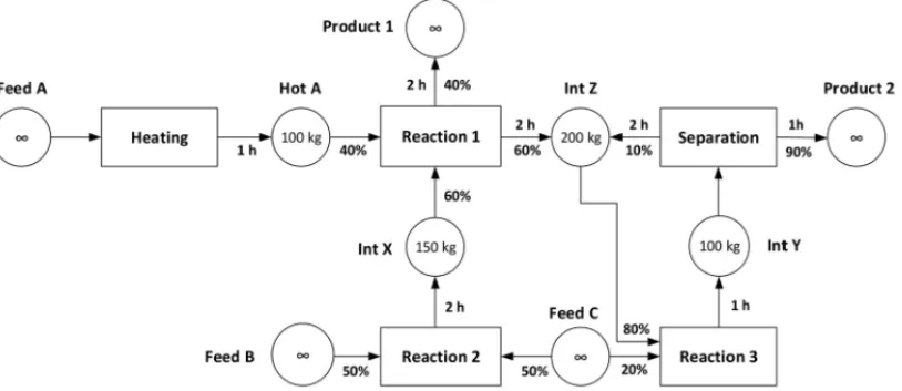
Figure 1, adapted from Kondili et al. (1993), illustrates the flexibility of STN on a petrochemical process with 9 states, 5 tasks and 1-hour discrete time slots. A storage capacity, sometimes unlimited, is indicated in each state. The percentages before a task define the proportions of the recipe, while the ones after a task specify the output yields. These percentages are implicitly equal to 100% when omitted, for instance for the tasks with a single input state.
Figure 1– Example of state-task network (adapted from Kondili et al., 1993).
We can notice that the STN can model tasks with multiple inputs and outputs (Reaction 1), loops (Reaction 3→Intermediate Y→Separation→Intermediate Z→Reaction 3), and processing times. For instance, the input products consumed by Reaction 2 in periodt yield a new product available on output in periodt+2. Note that changing a single characteristic of a product (state) makes it another product, e.g., “Feed A” becomes “Hot A” after heating.
Moreover, limited resources can be added. E.g., Kondili et al. (1993) mention for Figure 1 one heater (capacity 100 kg) for the “Heating” task, two reactors (80 and 50 kg), usable for the three tasks “Reaction 1”, “Reaction 2” and “Reaction 3”, and one distillation column for the “Separation” task.
Last but not least, the same authors show that a MILP can be generated from the STN, to deter-mine the timing of operations for each resource and the product flows through the network, so as to optimize a given objective function. All these features make the STN a powerful modeling tool for multi-period planning problems over discretized time horizons. Only simulation models can be more precise, but it is difficult to use them for optimization purposes.
3.2 Application to biomass supply chains and example
• Transportation tasks are added, the product before and after such tasks giving two distinct states.
• The final product (heat) is also considered as a state.
• Humidity is an additional attribute associated with the states.
• Tasks can be period-specific, e.g., the ambient drying rate is higher in August than in January.
• Utilities (manpower, gasoil, etc.) are defined for each processing unit to deduce CO2 emissions.
Samsatli et al. (2015) added another feature in their Resource-Technology Network (RTN). The RTN is in fact similar to the STN (the resources correspond to the STN states and the technologies to the STN tasks) but it becomes possible to select different modes for each technology.
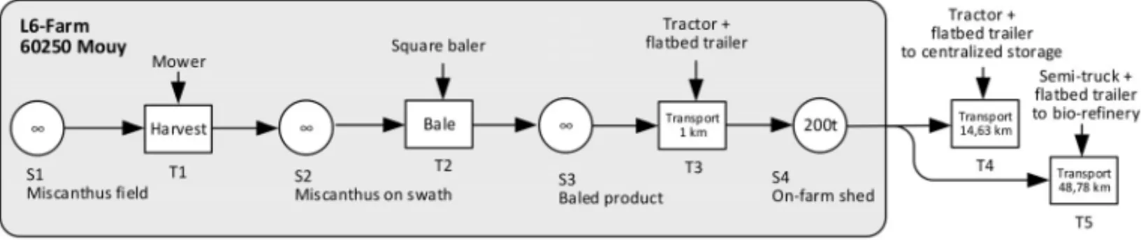
Figure 2 shows how a more complex supply chain like the one considered in our study can be represented as an STN. We add to the basic STN an upper level, the geographical locations, to model the set of states and tasks of each important site (gray rectangles). Three locations are considered: one farm producing rape (colza), one centralized storage with one silo for seeds plus one platform for bales, and one refinery with buffer stocks. The sites are composed of statesSe (stocks in a broad sense, including the rape fieldS1) and tasksTi. Each state contains a single productPk and is either a cultivated field, a work in process (like the straw on swath) or a true stock (silo for instance).
Only one crop is considered to keep the figure readable, but it is easy to add other crops. The whole rape (product P1) is cut by a combine harvester (taskT1) which yields three products: seeds (product P2), chaff (small particles, P3) and straw (stalks, P5). Each product is defined by a crop of origin (here, rape only), a crop part (seeds, chaff, straw), a presentation (bulk or square bales) and a moisture content.
The seeds are discharged in a trailer drawn by a tractor and brought immediately to the silo. The straw, available after 3 days of drying on swath, is packed in square bales using a tractor pulling a baler. These bales temporarily placed on the ground are either kept in a shed on the farm or sent to the refinery by a semi-trailer truck. The chaff is collected by the harvester in a special compartment which is emptied on the ground, giving a loaf which is then taken over by a square baler equipped with a special feeder. Chaff bales are carried by a tractor with a flatbed trailer, to be stored with the straw in the same shed. Then the same transport mode transfers the straw and chaff bales to the platform of the storage site. Finally, semi-trailers transport the products from the on-farm shed and the centralized storage to the buffer stocks of the refinery.
Fi
gur
e
2
–
E
xam
p
le
of
st
at
e-ta
sk
net
w
or
k
(STN
)
fo
r
a
si
m
p
le
suppl
y
c
hai
n
w
ith
one
fa
rm
,
one
cent
ral
ized
st
or
age
a
nd
oe
bi
or
efiner
y
on the other arcs. The refine-task is particular because its inflows (biomass demands) are given period per period: the percentages are not mentioned since they depend on the period.
The only notable wait is the passive drying of the straw on the ground (3 days) on exit from the harvesting task. This drying could also be modeled by a dedicated task. For the other tasks, there is no waiting time, which means that the inputs consumed in periodtare transformed into output products which can be used in the same period.
This example shows that the STN describes well the structure of the supply chain and its different activities. However, this graphical representation cannot be directly interpreted by a computer and many auxiliary data must be added, for instance the number of periods of the planning horizon, the length of a period in days, the costs and throughputs of equipment, the density of the different products to compute their transported volumes, etc. The role of the data model presented briefly in the next section is to encode the STN and all other required data as database tables.
4 DATA MODEL
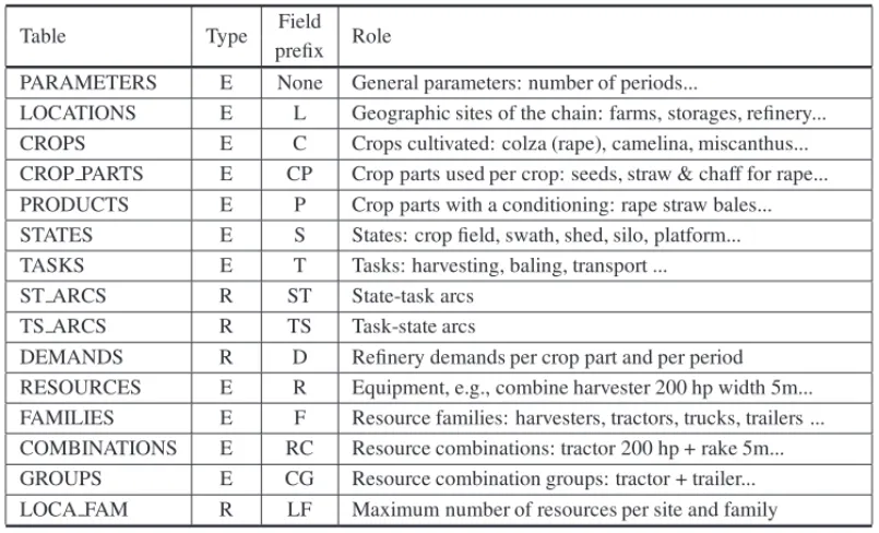
The purpose of this section is to explain, without entering into details, how the STN and all aux-iliary data can be structured efficiently as a set of database tables. Indeed, the data management layer is a critical component in optimization software, although it is often under-estimated in OR papers. We first present the list of tables used, the special way in which resources (equipment) are handled, and the list of data symbols from which the mathematical model of Section 5 is automatically generated.
4.1 Tables used
We selected theentity-relationshipapproach to analyze data. An entityis a set of things or persons sharing common properties, calledattributesorfields. Arelationshipdescribes the way the entities are linked. For instance, states and tasks represent two entities while state-to-task arcs constitute a relationship, more precisely a subset of the cross product of states and arcs. A relationship may have its own attributes, for instance an arc may have a length and a transported product.
Entities and relationships can be implemented as a set of tables stored in a database. We selected Excel, which is simpler and lighter than a true database management system. Each entity gives one Excel worksheet with one column per attribute and one row for each member (record) of the entity. Theidentifier(ID) orkeyis a mandatory attribute to identify each member of an entity unambiguously. All tables for one run of the model are stored in one Excel workbook. The user can evaluate different scenarios by modifying existing workbook or creating new ones.
is defined by one plant of origin, one part of this plant, and one form (e.g., bulk, bales, or pellets). The other worksheets describe the resource management system, described in Section 4.2. Such a data model is very flexible and new attributes can be easily added in each entity.
Table 1– List of worksheets (type E: implementing one entity, type R: one relationship).
Table Type Field Role
prefix
PARAMETERS E None General parameters: number of periods...
LOCATIONS E L Geographic sites of the chain: farms, storages, refinery... CROPS E C Crops cultivated: colza (rape), camelina, miscanthus... CROP PARTS E CP Crop parts used per crop: seeds, straw & chaff for rape... PRODUCTS E P Crop parts with a conditioning: rape straw bales... STATES E S States: crop field, swath, shed, silo, platform... TASKS E T Tasks: harvesting, baling, transport ...
ST ARCS R ST State-task arcs
TS ARCS R TS Task-state arcs
DEMANDS R D Refinery demands per crop part and per period RESOURCES E R Equipment, e.g., combine harvester 200 hp width 5m... FAMILIES E F Resource families: harvesters, tractors, trucks, trailers ... COMBINATIONS E RC Resource combinations: tractor 200 hp + rake 5m... GROUPS E CG Resource combination groups: tractor + trailer... LOCA FAM R LF Maximum number of resources per site and family
4.2 Resource management system
Our resource management system deserves some explanations. We callresourcesthe motorized equipment (harvesters, tractors, trucks...) and their accessories (rakes, balers, trailers...) used by the tasks. The table RESOURCES contains various commercial models with their characteristics, e.g., the productivity in hectares per hour (for a harvester), or the average speed (for a truck).
The resource families(FAMILIES worksheet) are categories of equipment with similar func-tions but which do not refer to specific models. Examples of families are mowers, combine harvesters, balers, trucks, farm trailers (drawn by a tractor), truck trailers, etc. Families serve in the LOCA FAM worksheet to limit the number of equipment which can be employed on each site, for example no more than two tractors on a farm. Each tractor can be any commercial model defined in RESOURCES.
the size of its trailer. The combinations have the same attributes as the resources but, because of special cases like our tractor example, only an expert in agricultural machinery can specify which combinations are possible and compute their attribute values, in order to fill the worksheet COMBINATIONS.
Finally, the combination groupsor generic combinations(worksheet GROUPS) play for the combinations the same role as the families for the resources: the exact characteristics are not specified. For example, a 200 hp tractor with a 15-ton flatbed trailer is a resource combination belonging to the combination group “tractor + trailer”.
In fact, the state-task graph specifies one group for each task, so the optimization module is free to choose any combination of real equipment in COMBINATIONS. The resource level is mainly used to cumulate the working hours of each selected equipment (since the same machine can be used by several tasks and in several combinations) and estimate fleet size.
4.3 Data and variables used by the mathematical model
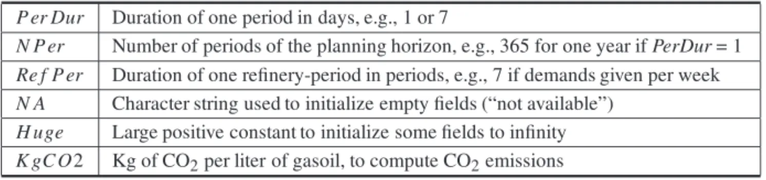
The data contained in the Excel workbook are listed below. The database contains other fields not described here, e.g., to format the results (full site names) or prepare the distance matrix (GPS co-ordinates). The general parameters listed in Table 2, like the number of periods, are loaded from worksheet PARAMETERS. As refinery demands are often specified per week or half-month, we introduce a longer periodRe f Perfor the refinery. Its use is explained in subsection 5.3.
Table 2– Data from worksheet PARAMETERS.
P er Dur Duration of one period in days, e.g., 1 or 7
N P er Number of periods of the planning horizon, e.g., 365 for one year ifPerDur= 1 Re f P er Duration of one refinery-period in periods, e.g., 7 if demands given per week N A Character string used to initialize empty fields (“not available”)
H uge Large positive constant to initialize some fields to infinity K gC O2 Kg of CO2per liter of gasoil, to compute CO2emissions
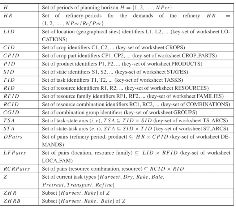
Table 3– Indexing sets.
H Set of periods of planning horizonH= {1,2, . . . ,N P er}
H R Set of refinery-periods for the demands of the refinery H R = {1,2, . . . ,N P er/Re f P er}
L I D Set of location (geographical sites) identifiers L1, L2, ... (key-set of worksheet LO-CATIONS)
C I D Set of crop identifiers C1, C2, ... (key-set of worksheet CROPS)
C P I D Set of crop part identifiers CP1, CP2, ... (key-set of worksheet CROP PARTS) P I D Set of product identifiers P1, P2, ... (key-set of worksheet PRODUCTS) S I D Set of state identifiers S1, S2, ... (keys-set of worksheet STATES) T I D Set of task identifiers T1, T2, ... (key-set of worksheet TASKS)
R I D Set of resource identifiers R1, R2, ... (key-set of worksheet RESOURCES) R F I D Set of resource family identifiers RF1, RF2, ... (key-set of worksheet FAMILIES) RC I D Set of resource combination identifiers RC1, RC2, ... (key-set of COMBINATIONS) CG I D Set of combination group identifiers (key-set of worksheet GROUPS)
T S A Set of task-state arcs(i,e),T S A⊆T I D×S I D(key-set of worksheet TS ARCS) ST A Set of state-task arcs(e,i),ST A⊆S I D×T I D(key-set of worksheet ST ARCS) D P air s Set of pairs (refinery period, product)⊆ H R×C P I D (key-set of worksheet
DE-MANDS)
L F P air s Set of pairs (location, resource family)⊆ L I D× R F I D (key-set of worksheet LOCA FAM)
RC R P air s Set of pairs (resource combination, resource)⊆RC I D×R I D Z Set of current task types{H arvest,Dr y,Rake,Bale,
Pr etr eat,T r ans por t,Re f i ne} Z H R Subset{H arvest,Rake}ofZ Z H R B Subset{H arvest,Rake, Bale}ofZ
Note that a few indexing sets do not correspond to worksheets listed in Table 1. RC R Pair s is required to define the different resources involved in each resource combination, while the last sets as fromZare introduced to improve model readability.
5 MATHEMATICAL MODEL
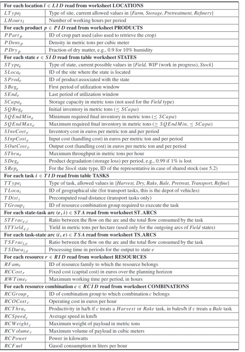
Table 4– Data arrays indexed over the sets of Table 3.
For each locationl∈L I Dread from worksheet LOCATIONS
L T y pel Type of site, current allowed values in{Farm, Storage, Pretreatment, Refinery}
L H our sl Number of working hours per period
For each productp∈P I Dread from worksheet PRODUCTS P Par tp ID of crop part used (also used to retrieve the crop)
P Densp Density in metric tons per cubic meter
P Dr yp Fraction of dry matter, e.g., 0.9 for 10% humidity
For each statee∈S I Dread from table worksheet STATES
S T y pee Type of state, current possible values in{Field, WIP(work in progress),Stock}
S Locae ID of the site where the state is located
S Pr ode ID of product associated with the state
S Bege First period of utilization window
S E nde Last period of utilization window
SCa pae Storage capacity in metric tons (not used for theFieldtype)
S Q Bege Initial inventory in metric tons (≤SCa pa)
S Q E nd M ine Minimum required final inventory in metric tons (≤SCa pa)
S Q E nd M axe Maximum required final inventory in metric tons (≥S Q E nd M in,≤SCa pa)
S I nvCoste Inventory cost in euros per metric ton and per period
S I npCoste Input cost (handling cost) in euros per metric ton and per period
S OutCoste Output cost (handling cost) in euros per metric ton and per period
S T hr ue Maximum throughput in metric tons per hour
S Dege Product degradation (storage loss) per period, e.g., 0.99 if 1% is lost
S Repe For theStockstate type, ID of the representative in case of shared stock (see 5.2)
For each taski∈T I Dread from table TASKS
T T y pei Type of task, allowed values in{Harvest, Dry, Rake, Bale, Pretreat, Transport, Refine}
T Locai ID of geographical site (for transport tasks, this is the depot of vehicles)
T Disti Precomputed road distance (transport tasks only)
T Gr oupi ID of resource combination group required to execute the task
For each state-task arc(e,i)∈ST Aread from worksheet ST ARCS
S T F r ace,i Ratio between the flow on the arc and the total flow consumed by the task
S T Y ielde,i Yield in metric tons per hectare (used only for the outgoing arcs ofFieldstates)
For each task-state arc(i,e)∈T S Aread from worksheet TS ARCS
T S F r aci,e Ratio between the flow on the arc and the total flow consumed by the task
T S Dur ai,e Processing time in periods for the output to statee
For each resourcer∈R I Dread from worksheet RESOURCES RF amr ID of resource family to which the resource belongs
RCCostr Fixed cost (capital cost) in euros over the planning horizon
RW T imer Maximum working time per period, in hours
For each resource combinationc∈RC I Dread from worksheet COMBINATIONS RCGr oupc ID of combination group to which combinationcbelongs
RC OCostc Operating cost in euros per hour
RCT hr uc Productivity in ha/h ifctreats aH arvestorRaketask, in bales/h ifctreats aBaletask
RC S peedc Average speed in km/h
RCW eightc Maximum weight of payload in metric tons
RCV olumec Maximum volume of payload in cubic meters
RC Power Power in kilowatts
Table 4– (Continuation).
For each pair(w,k)∈D P ai r sread from worksheet DEMANDS
D Needw,k Demand for crop partkin refinery-periodw, in dry metric tons
For each pair(l,f)∈L F P ai r sread from worksheet LOCA FAM
L F N M axl,f Maximum number of resources from family f that can be employed on sitel
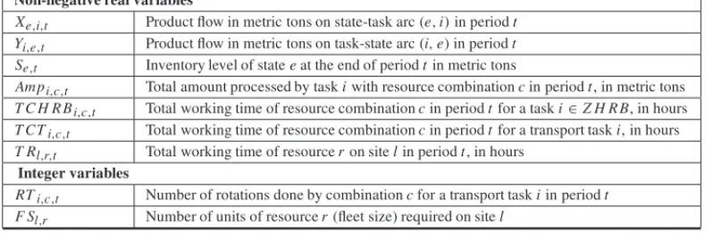
Table 5– List of variables.
Non-negative real variables
Xe,i,t Product flow in metric tons on state-task arc(e,i)in periodt
Yi,e,t Product flow in metric tons on task-state arc(i,e)in periodt
Se,t Inventory level of stateeat the end of periodtin metric tons
Am pi,c,t Total amount processed by taskiwith resource combinationcin periodt, in metric tons
T C H R Bi,c,t Total working time of resource combinationcin periodtfor a taski∈Z H R B, in hours
T CTi,c,t Total working time of resource combinationcin periodtfor a transport taski, in hours
T Rl,r,t Total working time of resourceron sitelin periodt, in hours
Integer variables
RTi,c,t Number of rotations done by combinationcfor a transport taskiin periodt
F Sl,r Number of units of resourcer(fleet size) required on sitel
5.1 Declaration of variables
A general principle is to restrict the indexing of variables listed in Table 5, to reduce model size. Inventory levels(Se,t), flows on state-task arcs(Xe,i,t), and task-state arcs (Yi,e,t)are defined only in the time windows when stateeis open, see constraints (1)-(3).
∀(e,i)∈ST A, ∀t∈ [S Bege,S Ende] : Xe,i,t ≥0 (1)
∀(i,e)∈T S A, ∀t ∈ [S Bege,S Ende] :Yi,e,t ≥0 (2)
∀e∈ S I D, ∀t∈ [S Bege,S Ende] :Se,t ≥0 (3)
For each taskiand each periodt, the variablesAmp(amount processed) are defined only for the resource combinationscwhich may be used by the task, see constraints (4). TheRe f inetask of the refinery is not concerned since its amounts processed are fixed and equal to the demands.
∀i ∈T I D|T T ypei =“Re f ine′′, ∀c∈ RC I D|RCGr ou pc=T Groupi, ∀t ∈ H : Ampi,c,t ≥0
(4)
In constraints (5), the integer variables for the number of vehicle rotations are generated only for transport tasks and resource combinations usable by each task.
∀i ∈T I D|T T ypei =“T rans port′′, ∀c∈ RC I D| RCGroupc=T Groupi, ∀t ∈H : RTi,c,t ∈N
Finally, the integer number of units of resourcerto purchase for geographical site (location)lis defined only for the resource families allowed on the site.
∀l ∈L I D,∀r ∈ R I D|(l,R Famr)∈L F Pairs : F Sl,r ∈N (6)
5.2 Inventory and flow constraints
Storage capacity. We added an attributeS Repeto model a group of states as one shared storage, for instance a platform storing bales of different products. In the data, one representativer is defined for the group and all memberseof the group (evenr) are such thatS Repe =r. A non-shared storageehas no representative:S Repe=N A. Storage capacity constraints are generated only if a limited capacity is specified. Constraints (7) concern non-shared stocks. Constraints (8) for shared stocks are generated only for representatives, i.e., statesesuch thatS Repe=e.
∀e∈S I D|SCapae<H uge and S Repe=N A, ∀t ∈ [S Bege,S Ende] :Se,t≤ SCapae
(7)
∀e∈ S I D|SCapae<H uge and S Repe =e,
∀t∈ [S Bege,S Ende] : u∈S I D|S Repu=eSu,t ≤ SCapae
(8)
Inventory balance equations. They take degradations into account. Constraints (9) concern the first period of the opening window and the initial inventory. Constraints (10) are for the other periods.
∀e∈S I D : Se,S Bege
=S Q Bege·S Dege+(i,e)∈T S A Yi,e,S Bege−(e,i)∈S T A Xe,i,S Bege
(9)
∀e∈ S I D, ∀t∈ ]S Bege,S Ende] :Se,t
=Se,t−1·S Dege+
(i,e)∈T S A Yi,e,t−(e,j)∈S T A Xe,j,t
(10)
Definition of flows on task outgoing arcs. Constraints (11) translate one property of STN net-works: the flow on a task outgoing arc(i,e)is equal in each periodtto a fractionT S Fraci,eof the total input flow consumedT S Duraieperiods before.
∀(i,e)∈T S A, ∀t ∈ [S Bege,S Ende] |t−T S Duraie ≥1:Yi,e,t
=T S Fraci,e·(u,i)∈S T AXu,i,t−T S Duraie
(11)
Definition of flows on task incoming arcs. Constraints (12) specify the fraction of the total input flow taken on each incoming arc. For theRe f inetask, they are replaced by demand constraints, see 5.3.
∀(e,i)∈ST A|T T ypei =“Re f ine′′, ∀t∈ [S Bege,S Ende] : Xe,i,t
=ST Frace,i·(e,j)∈S T A|j=i Xe,j,t
(12)
can be less than 1 if the yield is not perfect. The resulting flow appears on outgoing arcs(i,u), T S Durai,u periods later. For the refinery, these constraints have a different form explained in 5.3.
∀i ∈T I D|T T ypei =“Re f ine′′, ∀t ∈H : (e,i)∈S T A|t∈ [S Beg
e,S E nde]Xe,i,t ·
(i,u)∈T S A T S Fraci,u=
(i,u)∈T S A|t∈[S Begu,S E ndu−T S Dura(i,u)]Yi,u,t+T S Dura(i,u)
(13)
Final inventory constraints. They are generated for the last period of the opening period of each stockeif a final stock is specified. Constraints (14) for minimum final inventories are mainly used for the input stocks of the refinery, to chain successive years without having to stop activities. Constraints (15) deal with maximum final inventories. For instance,S Q End Maxe =0 is used to empty a stock after the last periodS Endeof its window.
∀e∈S I D|S Q End Mine>0 :Se,S E nde ≥S Q End Mine (14)
∀e∈S I D|S Q End Maxe<H uge: Se,S E nde ≤ S Q End Maxe (15)
Maximum reception capacity of storage states. Constraints (16) deal with storage states like silos. They have a maximum reception capacityST hrue, in metric tons per hour, to be multiplied by the number of opening hours per period of the geographical site containing the state.
∀e∈S I D|ST ypee=St ock,
∀t ∈ [S Bege,S Ende] : (i,e)∈T S A Yi,e,t ≤ST hrue·L H ours[S L ocae]
(16)
5.3 Demand satisfaction constraints
The supply chain is analyzed over base-periods of 1 or 7 days. Refinery demands use a longer period, in general 1 or 2 weeks, equal toRe f Per base-periods. Moreover, they are expressed in dry tons of some crop parts. The exact products are not imposed, e.g., a demand of 185 dry tons of rape straw can be satisfied using 100 tons of bales with 10% humidity and 100 tons of pellets with 5%.
As refinery production variations are unknown, we assume that the need in dry tons for crop part kin refinery periodwis consumed at a constant rate in each base-period. For instance, a demand of 70 tons in weekw is consumed at a rate of 10 tons/day. Note that this does not imply to receive the same amounts daily, since the refinery has input stocks for 2 weeks of production, on average.
∀i ∈T I D|T T ypei =“Re f ine′′,∀(w,k)∈ D Pairs, ∀t ∈ [(w−1)·Re f Per+1, w·Re f Per] :
(e,i)∈S T A|P Part[S Prode]=kP Dr y[S Prode] ·Xe,i,t
=D N eedw,k/Re f Per
(17)
are requested a few weeks or months per year. The sum cumulates the flows of productsXe,i,t (converted in dry tons) for crop partk, from the input stocks in each base-period of the refinery period. It must be equal to the uniform consumptionD N eedw,k/Re f Per in the refinery period.
5.4 Resource management constraints
The principles of our resource management system were introduced in subsection 4.2. Recall that in worksheet TASKS a group of resource combinations is specified for each taski, e.g., “one tractor + one trailer”. The task may use several combinations in the same group, e.g., one 200-hp tractor with a 6-meter trailer, plus one 240-hp tractor with a 8-meter trailer.
Constraints (18) mean that the total input flow of each taski in each periodtmust be processed by the resource combinationscallowed for this task.
∀i ∈T I D|T T ypei =“Re f ine′′,∀t ∈ H :
c∈RC I D|RC Grou pc=T Groupi Ampi,c,t =
(e,i)∈S T AXe,i,t
(18)
The next step is to convert the amounts processed in resource combination working times. For farm tasksH arvest, RakeandBale(set of task typesZ H R B), constraints (19) compute the variablesT C H R Bi,c,t (working time of combinationcfor farm taski en p´eriodet), which are necessary to count the operational costs of farm equipment (Farm O pCost s) in the objective function. We have two cases because the productivities RT hru are in hectares per hour for H arvest and Rake(set Z H R) tasks but in bales per hour forBaletasks. We get metric tons per hour using the crop yield forH arvest andRaketasks, and the volume of a bale and product density forBaletasks.
∀i∈T I D|T T ypei ∈ Z H R B,∀c∈ RC I D |RCGr oupc=T Groupi,∀t ∈ H :
IfT T ypei ∈Z H R
then: T C H R Bi,c,t =
Amp i,c,t
(e,i)∈S T ARCT hruc·ST Y ielde,i
else: T C H R Bi,c,t =
Amp i,c,t
(e,i)∈S T ARCT hruc·RCV olumec·P Dens(S Prode)
(19)
In constraints (20), the working timeT CT i,c,t for a transport task is based on the number of vehicle rotationsRTi,c,t, the distance travelledDisti and the average speed of the combination RC S peedc.
∀i ∈T I D|T T ypei =“T rans port′′,
∀c∈ RC I D |RCGr oupc=T Groupi,
∀t ∈ H : T CTi,c,t =
2·T Disti·RTi,c,t RC S peedc
(20)
for H arvest, Rakeand Baletasks from the ones forT rans port tasks, because a tractor (for instance) can be used by all these tasks.
∀l ∈L I D,∀r ∈R I D|(l, R Famr)∈L F Pairs,
∀t∈ H :T Rl,r,t =c∈RC I D|(c,r)∈RC R Pairs (i∈T I D|T T y pei∈Z H RB and RC Gr oup
c=T Groupi and T Locai=lT C H R Bi,c,t+
i∈T I D|T T y pei=“Transport′′ and RC Grou p
c=T Groupi and T Locai=lT CTi,c,t)
(21)
To help the solver, simple bounds are applied to the integer variables RTi,c,t, the number of rotations in period t for the resource combinationcused by task i, e.g., a semi-truck with a road trailer. In the lower bounds of constraints (22), Ampi,c,t is divided by the minimum of vehicle capacity and maximum weight (resulting from vehicle volume and product density). As the product is defined for states but not for tasks, the sum is used to get the stateeof origin, which is unique for a transport task. The quotient cannot be rounded up to the closest integer if we wish to keep the model linear.
∀i ∈T I D|T T ypei ∈Z T, ∀c∈ RC I D|RCGr ou pc=T Groupi,∀t∈ H :
RTi,c,t ≥
Ampi,c,t
min(RCW eightc, (e,i)∈S T ARCV olumec·P Dens(S Prode))
(22)
RTi,c,t cannot exceed the previous lower bound plus 1. For instance, if the quotient in (22) is 6.3, the integer variable RTi,c,t must be greater than 6.3 and less than 7.3: the solver has no choice and sets it to 7.3. If the quotient is integer, say 6, the solver has the choice, but only among two values, 6 and 7.
∀i ∈T I D|T T ypei ∈ Z T, ∀c∈ RC I D|RCGr ou pc =T Groupi,∀t ∈H :
RTi,c,t ≤
Ampi,c,t
min(RCW eightc , (e,i)∈S T ARCV olumec·P Dens(S Prode))
+1 (23)
In constraints (24)-(25), the number of units of resource r required on sitel, F Sl,r, can be bounded using the maximum resource working time and the number of opening hours of the site (per period).
∀l∈ L I D, ∀r∈ R I D|(l,R Famr)∈L F Pairs,
∀t ∈ H: F Sl,r ≥
T Rl,r,t
min(RW T imer , L H oursl) (24)
∀l∈ L I D, ∀r∈ R I D|(l,R Famr)∈L F Pairs,
∀t ∈ H: F Sl,r ≤
T Rl,r,t
min(RW T imer , L H oursl)+1 (25)
Finally, the total number of resource units per family is limited via constraints (26). These constraints were introduced after preliminary tests where all fields were harvested in too few periods, implying an unrealistic number of combine harvesters.
5.5 Objective function
Over the planning horizon, the objective function defined by Equation (27) includes operational costs of farm equipment (FarmCost s), transport costs (T ranCost s), fixed costs (capital costs) of resources (FixedCost s), inventory costs (I nvCost s), and handling costs (H andCost s).
MinZ =FarmCost s +T ranCost s+FixedCost s+I nvCost s+H andCost s (27)
In Equation (28),FarmCost s concerns resource combinations for H arvest, Rakeand Bale tasks (setZ H R B), the transports in the farms being counted with other transports inT rans O p -Cost s. It is derived from working timesT C H R Bi,c,t computed in constraints (19). The first sum includes each task i with a typeT T ypei is in Z H R B. The second considers only the combinationscof the resource combination set(RC I D) which have the group recommended for the task(RCGr oupc=T Groupi).
FarmCost s =i∈T I D|T T y pe
i∈Z H RB
c∈RC I D|RC Grou pc=T Groupi
×t∈HT C H R Bi,c,t·RC OCostc
(28)
T ransCost s is deduced in Equation (29) from working times T CTi,c,t computed in con-straints (20).
T ranCost s =i∈T I D|T T y pe
i=“T ransport′′
c∈RC I D|RC Gr oupc=T Groupi
×t∈HT CTi,c,t·RC OCostc
(29)
FixedCost s is computed in equation (30) from variables F Sl,r computed in constraints (24)-(26).
FixedCost s =l∈L I Dr∈RI D|(l,RF am
r)∈L F PairsF Sl,r ·RCCostr (30)
A storage cost is applied to the amount contained in each stateeat the end of each periodt. In general,Field andW I Pstates have no storage cost. Some true storages like silos can be used only a few weeks or months per year for the biorefinery. The rest of the time, they are reserved to other activities like cereal production. Hence, the storage costs in equation (31) are counted only in the opening window[S Bege,S Ende].
I nvCost s =e∈S I Dt∈[S Beg
e,S E nde]S I nvCoste·Se,t (31)
Finally, the handling costs (32) are applied to the amounts of products entering or leaving a stor-age. They avoid detailing the numerous little resources involved: band conveyors and aspirators of grain silos, forklifts used to stack bales, etc.
H andCost s=(i,e)∈T S At∈[S Beg
e,S E nde]S I npCoste·Yi,e,t
+(e,i)∈S T At∈[S Beg
e,S E nde]S Out Coste·Xe,i,t
5.6 Derivation of energy consumptions and CO2emissions
Environmental criteria are important to appraise a biomass supply chain. The following equations are used to derive the energy consumption and the CO2 emissions from the optimal solution to the mathematical model. They can also be included with adequate weights in the objective function (27).
For each resource combination is given a power RC Power in kW. In general it corresponds to the motorized component of the combination, e.g., the tractor for a “tractor + baler” com-bination. It can be also the power of electric equipment such as an oven or a press in a pre-treatment/densification site. In Equation (33), the total energy consumption in kW×h is simply deduced from the powers RC Power of resource combinations and their working times, i.e., T C H R Bi,c,t for harvesting equipment andT CTi,c,t for transport vehicles.
Energy=i∈T I Dc∈RC I D|RC Grou p
c=T Groupi
×t∈H(T CT i,c,t +T C H R B i,c,t)·RC Power
(33)
Equation (34) for CO2emissions is almost as simple. Indeed, we know for each resource com-bination the gasoil consumptionR Fuel in liters per hour, while table PARAMETERS indicates the number of kilograms of carbon dioxide emitted per liter of gasoil,K gC O2 (nearly 2.6 kg/l).
C O2=i∈T I Dc∈RC I D|RC Grou p
c=T Groupi
×t∈H(T CT i,c,t +T C H R Bi,c,t)·RC Fuel ·K gC O2
(34)
6 NUMERICAL EVALUATIONS ON REAL DATA
The effectiveness of our MILP model based on extensions and adaptations of state-task networks is demonstrated on a few numerical examples based on real data. Only the first example can be described completely, due to the large amount of data involved in the other tests.
6.1 First example
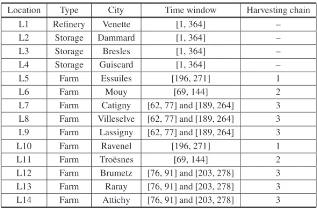
This case involves 10 production zones (“farms” in a broad sense) which cultivate rape (colza) and/or miscanthus and 3 centralized storage sites, at 50 km maximum from one local refinery close to the city of Compi`egne (60 km at the north of Paris). These sites are listed in Table 6.
The three first columns respectively give the location (geographical sites) identifiers, the site types and the municipalities. We selected a total demand of 50,730 metric tons/year of dry matter, a typical value for a local biorefinery. Rape yields three products (bulk seeds, straw bales, chaff bales) while miscanthus provides straw bales only.
Table 6– Data for locations and their attributes.
Location Type City Time window Harvesting chain
L1 Refinery Venette [1, 364] –
L2 Storage Dammard [1, 364] –
L3 Storage Bresles [1, 364] –
L4 Storage Guiscard [1, 364] –
L5 Farm Essuiles [196, 271] 1
L6 Farm Mouy [69, 144] 2
L7 Farm Catigny [62, 77] and [189, 264] 3
L8 Farm Villeselve [62, 77] and [189, 264] 3
L9 Farm Lassigny [62, 77] and [189, 264] 3
L10 Farm Ravenel [196, 271] 1
L11 Farm Tro¨esnes [69, 144] 2
L12 Farm Brumetz [76, 91] and [203, 278] 3
L13 Farm Raray [76, 91] and [203, 278] 3
L14 Farm Attichy [76, 91] and [203, 278] 3
Table 7– Annual demands for each crop part.
Crop Product Annual demand
Seeds (bulk) 17,690 Rape Straw (bales) 14,120 Chaff (bales) 6,920 Miscanthus Straw (bales) 12,000
Each farm grows rape and/or miscanthus. The harvesting chain and harvesting windows applied to each farm are given in the two last columns of Table 6. Chain 1, used by farms 5 and 10 which produce rape only, is identical to the chain already depicted in Figure 2. Chain 2 (see Fig. 3 for an example) is employed in farms 6 and 11 which cultivate miscanthus only. The other farms produce both crops using chain 3, a combination of chains 1 and 2 with a shared on-farm storage for all baled products (rape straw, rape chaff and miscanthus). The earliest windows, ending at period 144 or before, are related with miscanthus, harvested in March-April. Those beginning as from period 189 (beginning of July) concern rape. The windows vary slightly depending on soils but all end beg-October. The refinery and centralized storages (sites L1-L4) are open all over the year.
It is assumed that each farm may ship biomass to the closest storage site and to the refinery. Real distances by road were calculated using the MapPoint software from Microsoft. Data for the equipment were found in agricultural databases, see for instance [18].
Figure 3– Harvesting chain number 2 for miscanthus.
portable PC with a 2.7 GHz Intel Core i7-3740 QM processor, 16 GB of RAM, and Windows 7 Professional.
Although the number of farms (10) looks modest, the model is already huge, due to the number of periods and the number of states and tasks in the STN. For instance, even a farm growing rape only requires 8 states and 11 tasks, with associated decision variables (flows and stocks) in-dexed over 364 periods. The whole model has in fact 588,304 constraints and 500,094 variables, including 91,437 integer variables. The pre-solver of CPLEX reduces it to 87,445 constraints and 94,883 variables, including 31,575 general integer variables and 9,826 binary variables. The binary variables are visibly used to replace the number of vehicle rotations and the number of resource units when they have small upper bounds. The overall running time is reasonable: an optimal solution costing 4,829,586 euros is obtained in less than 3 minutes (164 seconds).
Figure 4 shows the breakdown of the expenses. The fixed costs of equipment are included in the harvesting part. Storage costs represent 59%, while they are often under-estimated in the litera-ture. In fact, this percentage is normal because the harvest periods are short (about 15 days for each of the two crops), while the refinery consumes biomass throughout the year: it is therefore necessary to build up important stocks. In particular, initial stocks must be sufficient to supply the refinery before the harvesting periods for miscanthus and (later) rape, to avoid infeasibility.
6.2 Simplifications for large instances
The model can be solved up to 80 farms and 20 centralized storage sites, over one year divided into 52 weeks. Such a size is already respectable but we found one example with 100 farms/25 storages which cannot be solved over 52 weeks: the branch-and-bound of CPLEX reports an “out of memory” error. The problem clearly comes from the large number of integer variables, F Sl,r andRTi,c,t.
The model computes the number of machines F Sl,r to buy for each site. This leads to a total cost where equipment investments are predominant. In reality, a farmer uses also his machines for other crops not asked by the refinery and may help other farmers or be helped. So, it is difficult to isolate the equipment cost fraction related to the refinery supply chain. The French Chambers of Agriculture regularly publish tariffs to invoice such exchanges [18]. The main interest is to pro-vide costs which include everything, even maintenance and equipment amortization. It becomes possible to optimize a total cost, composed of the resource working times of constraints (19)-(20), multiplied by the hourly tariffs. The modification of the objective function is straightforward and variablesF Sl,r can be suppressed. However, if the user wishes so, it is still possible to derive the equipment required on each site from the optimal solution, using constraints (24)-(26).
The numbers of vehicle rotationsRTi,c,t used to compute transport costs can also be avoided using a simpler system in tons×km, often applied when a refinery subcontracts its transports. The French Federation of Road Transport (FNTR) (http://www.fntr.fr) gives formulas for various trucks.
We have solved again the 10-farm case with 364 days to evaluate the impact of these simplifica-tions. The numbers of variables and constraints are roughly divided by 2 and, obviously, there are no more integer variables. Before the pre-solve, the model has 265,245 variables and 212,760 constraints. The pre-solver goes down to 26,580 variables and 9,791 constraints. The running time drops from 164 seconds to less than one second. The solution obtained is very similar to the one of the complete model, with an important cost difference equal to the equipment fixed costs since they are no longer counted. Looking at the other costs, a marginal difference of only 0.53% can be observed.
These simplifications also allowed to solve the case with 100 farms, 25 storages and 52 weeks which raised an “out of memory” error for the complete model. The simplified MILP has 162,074 variables and 203,721 constraints. Once pre-solved, only 8,339 variables and 5,839 constraints remain. The running time reaches 8,158 seconds (2 hours 1/4) but this duration is acceptable for strategic studies. By dichotomy, we were able to solve instances with 150 production zones, but not more.
5. The stock-states before leaving the farm must be kept, otherwise the macro-task would be connected to transport tasks (remember that two tasks cannot be directly connected in an STN).
Macro-tasks are similar to the tasks considered before, with three important differences.
• A classical task may use one resource combination only, while a macro-task may involve several combinations, in fact, all resource combinations required by the aggregated tasks.
• In a classical task, the resource combination used processes 100% of the total input flow, while in a macro-task it can be applied to sub-products. For instance, Figure 2 shows that rape yields 18% of chaff, which explains that the combination “tractor + square baler” used to bale chaff in Figure 5 treats only 18% of the total amount of rape harvested on input.
• Waiting times are still possible for some outputs, see the straw released after 3 days of passive drying in Figure 5, but feasible solutions with pauses inside the harvesting process are now excluded, e.g., when the farmer harvests during one day, stops the second day, and terminates the job the third day. However, we have never seen such useless breaks in the optimal solutions of the complete model and, anyway, they do not correspond to agricultural practices: indeed, due to meteorological uncertainties, farmers prefer to work continuously once they start harvesting.
The condensation of harvesting chains into macro-tasks must be done manually and carefully, but then the database and model modifications are relatively easy. The model encompassing all these simplifications, called “compact model” is applied to a large-scale case in the next subsection.
6.3 Large-scale example
To appraise the performance of the compact model, a large case was built after a long work to collect data and format them for our database. Although many detailed data at the farm level are protected in France by the statistical secret, the main results per municipality of the 2010 Agricultural Census are publicly available, including the number of farms, the cultivated area, and the dominating profile, e.g., “cereals and oilseed crops”, “viticulture”, etc.
Fi
gur
e
5
–
S
ta
te
-t
ask
n
et
w
o
rk
of
Fi
gur
e
2
af
te
r
the
in
tr
oduct
io
n
o
f
the
m
acr
o-ta
A partner of the research project has sent questionnaires to the operators of centralized storages, again within a maximum distance of 50 km to Compi`egne. The answers were typed in an Excel file giving the following data for 46 storage sites: kind of storage (silo or platform), capacities in tons for silos and square meters for platforms, storage costs, input and output costs, availability window in the year. Storage capacities vary from 200 to 60,000 tons. Each farm may send its products (seeds, straw bales and chaff bales from rape) to the nearest centralized storage, but not directly to the refinery. The planning horizon is one year subdivided into 52 weeks. The total refinery demand is 50,000 metric tons per year and road distances were computed again using MapPoint.
The resulting model contains 588,249 constraints and 574,795 variables. After a reduction to 4,801 constraints and 19,558 variables by the pre-solver, it is solved to optimality in less than one minute (47 seconds).
Our model and its results can be compared BioFeed (Shastri et al., 2011a). This closest model in the literature is more restrictive than ours, since it considers a single product from a single crop and a unique harvesting chain in three steps (harvest, rake, and bale). In Shastri et al. (2011b), BioFeed is applied to a switchgrass supply chain involving 31 farms, 1 centralized storage, and 1 biorefinery. The harvesting period of 120 days is divided into 15-day time steps. In the rest of the year, divided into 60-day time steps, flow variables for farm activities are not generated. The model requires 5,706 seconds of CPU time on a Dell PowerEdge 1900 server with 8 processors, a more powerful computer than our portable PC. So, although the instances compared differ substantially, it seems that our model can tackle larger supply chains, in a more flexible way, and in shorter CPU times.
7 CONCLUSION
A mixed integer linear programming (MILP) model was formulated to optimize biomass supply chains. The state-task network used to describe a chain is very flexible, since its allows to model in details farm activities, equipment selection, pretreatments, storages, and transports, for differ-ent crops and multiple products per crop, over a one-year planning horizon divided into days or weeks. The state-task network and other data such as resource characteristics are described in a database from which the mathematical model is automatically generated.