ISSN 0101-8205 www.scielo.br/cam
Numerical method, existence and uniqueness for
thermoelasticity system with moving boundary
M.A. RINCON1, B.S. SANTOS2 and J. LÍMACO2 1Instituto de Matemática, Universidade Federal do Rio de Janeiro
2Instituto de Matemática, Universidade Federal Fluminense
Rio de Janeiro, Brazil
E-mails: [email protected] / [email protected] / [email protected]
Abstract. In this work, we are interested in obtaining existence, uniqueness of the solution and an approximate numerical solution for the model of linear thermoelasticity with moving boundary. We apply finite element method with finite difference for evolution in time to obtain an approximate numerical solution. Some numerical experiments were presented to show the moving boundary’s effects for problems in linear thermoelasticity.
Mathematical subject classification: 35A05, 35A40, 65M60, 65M06.
Key words: thermoelasticity system; moving boundary; finite element method; finite differ-ence method.
1 Introduction
Let Qt =
(x,t)∈R2;α(t) <x < β(t),0<t<T be the non-cylindrical
domain with boundary
6t = [
0<t<T
{α(t), β(t)} × {t}
and consider the following problem:
(I)
∂2u ∂t2 −
∂2u ∂x2 +η1
∂θ
∂x =0, ∀(x,t)∈ Qt
∂θ
∂t −k ∂2θ ∂x2 +η2
∂2u
∂x∂t =0, ∀(x,t)∈ Qt,
u =θ =0, ∀(x,t)∈6t,
u(x,0)=u0(x), ∂u
∂t(x,0)=u1(x), θ (x,0)=θ0(x); α(0) <x < β(0).
Existence and uniqueness of linear and nonlinear elasticity in a bounded or an unbounded cylindrical domain, has been studied by several authors, among them, [4] and [5].
In this work, we will investigate existence, uniqueness and approximate so-lution of the problem (I). We will also show the influence of moving boundary
employing numerical examples. For this we consider the following hypotheses:
H1: α, β∈C2([0,T);R), with 0< γ0= min
0≤t≤Tγ (t), where γ (t)=β(t)−α(t),
H2: ∃k1∈R, such that,
0<k1<1− α′(t)+γ′(t)y2, for 0≤t≤T and 0≤ y≤1. H3: k>0, and η1.η2>0.
We will now consider a change of variables to transform the domainQt into a cylindrical domainQ. Observe that, when(x,t)varies in Qt the point(y,t)of
R2, withy =(x−α(t))/γ (t)varies in the cylinder Q=(0,1)×(0,T). Thus, we define the application
T : Qt → Q=(0,1)×(0,T)
(x,t)7→(y,t)=x−α(t) γ (t) , t
.
(1)
The applicationT belongs toC2and its inverseT−1is alsoC2. The
Doing the change of variable v(y,t) = u(α(t)+γ (t)y,t) and φ (y,t) = θ (α(t)+γ (t)y,t) and applying to the problema (I), we obtain the following
equivalent problem defined in a fixed cylindrical domain:
(II)
∂2v ∂t2 −
∂ ∂y
a1(y,t) ∂v ∂y
+a2(t) ∂φ ∂y
+a3(y,t)∂ 2v
∂y∂t +a4(y,t) ∂v
∂y =0, inQ
∂φ
∂t −b1(t) ∂2φ
∂y2 +b2(t) ∂2v
∂y∂t +b3(y,t) ∂φ ∂y
+b4(t)∂v∂y +b5(y,t)∂ 2v
∂y2 =0, inQ
v =φ =0; ∀(y,t)∈6,
v(y,0)=v0(y), ∂v
∂t(y,0)=v1(y),
φ(y,0)=φ0(y), for 0< y<1. where
b1(t)=k/γ (t)2, b2(t)=η2/γ (t) , b3(y,t)= −(α′(t)+γ′(t)y)/γ (t) , b4(t)= −γ′(t)/γ (t)2, b5(y,t)=b3(y,t)/γ (t) , a1(y,t)=1/γ (t)2−b3(y,t)2, a2(t)=η1/γ (t) , a3(y,t)=2b3(y,t) , a4(y,t)= −(α′′(t)+γ′′(t)y)/γ (t). Let(( , )), k ∙ kand( , ), | ∙ |, be respectively the scalar product and the norms inH01(0,1)andL2(0,1). We denote bya1(t, v, w)andb1(t, v, w)the bilinear
forms, continuous, symmetric and coercive, defined inH01(0,1)by
a1(t, v, w) =
Z 1 0
a1(y,t) ∂v ∂y
∂w ∂y d y,
b1(t, v, w) =
Z 1 0
b1(t)∂v ∂y
∂w ∂y d y.
(2)
2 Existence and uniqueness
We shall first establish the existence and uniqueness of problem (II) in Theorem 2
Theorem 1. Under the hypotheses(H1),(H2)and(H3)and given the initial data
{u0, θ0} ∈H01(0)∩H2(0), u1∈ H01(0),
there exist functions{u; θ} : Qt →R, solution of Problem(I)in Qt, satisfying
the following conditions:
1. u∈ L∞(0,T;H01(t)∩H2(t)), u′∈ L∞(0,T;H01(t)),
u′′∈ L∞(0,T;L2(t)),
2. θ ∈ L2(0,T;H01(t)∩H2(t)), θ′∈ L2(0,T;H01(t)).
Theorem 2. Under the hypotheses(H1),(H2)and(H3)and given the initial data
{v0, φ0} ∈H01(0,1)∩H2(0,1), v1∈ H01(0,1),
there exists functions{v; φ} : Q→R,solution of Problem(II)in Q, satisfying the following conditions:
1. v∈L∞(0,T;H01(0,1)∩H2(0,1)), v′∈ L∞(0,T;H01(0,1)), v′′ ∈L∞(0,T;L2(0,1)),
2. φ∈ L2(0,T;H01(0,1))∩H2(0,1), φ′ ∈L2(0,T;H01(0,1)).
Proof of Theorem 2. To prove the theorem, we introduce the approximate
so-lutions. LetT >0 and denote byVmthe subspace spanned by{w1, w2, ..., wm}, where{wν, λν;ν =1,∙ ∙ ∙m}are solutions of the spectral problem((wi, v))=
μ(wi, v), ∀v∈ H01(0,1).If{vm;φm} ∈Vm then it can be represented by
vm = m X
ν=1
dνm(t)wν(y), φm = m X
ν=1
Let us consider{vm;φm}solutions of the system of ordinary differential equa-tions,
(III)
(v′′m, w)+a1(t, vm, w)+a2
∂φm
∂y , w
+ a3∂v ′ m
∂y , w
+
a4∂vm ∂y , w
=0,
(φm′ , w)+b1(t, φm, w)+b2
∂vm′ ∂y , w
+
b3∂φm ∂y , w
+
2b4
∂vm
∂y , w
+
b5 ∂vm
∂y , ∂w
∂y
=0,
vm(0)=v0m →v0, in H01(0,1)∩H2(0,1),
vm′ (0)=v1m →v1 in H01(0,1),
φm(0)=φ0m →φ0 in H01(0,1)∩H2(0,1),
wherew ∈ Vm. The system (III) has local solution in the interval(0,Tm). To extend the local solution to the interval(0,T)independent ofm, the following
estimates are necessary:
A priori estimate
Takingw = v′m andw = φm in the equation (III)1and (III)2, respectively, we
get
1 2
d dt |v
′
m|2 + a1(t, vm, vm′ ) + a2 ∂φm
∂y , v ′
m
+ a3 ∂v′m
∂y , v ′
m
+ a4 ∂vm
∂y , v ′
m
= 0,
(4)
1 2
d dt |φm|
2
+ b1(t, φm, φm) + b2 ∂v′
m
∂y , φm
+ b3∂φm ∂y , φm
+ 2b4
∂vm
∂y , φm
+ b5 ∂vm
∂y , ∂φm
∂y
= 0.
Note that, we have the following relations:
a1(t, vm, vm′ ) = 1 2
d
dt a1(t, vm, vm)−
1 2
a1′∂vm ∂y ,
∂w ∂y , a2 ∂φm
∂y , v ′
m
= −ηη1 2
b2
∂v′
m
∂y φm
, a3∂v ′ m
∂y , v ′
m
= −γ ′ γ |v
′ m| 2, b3 ∂φm
∂y , φm
= 2γ′ γ|φm|
2,
b5∂vm ∂y ,
∂φm
∂y
≤ ckvmk2+ 1
2b1(t, φm, φm).
(6)
Multiplying (4) by(η2/η1), adding it to (5) and using (6) we have η2
2η1 d dt
|vm′ |2+a1(t, vm, vm)+
η1 η2|
φm|2
+b1(t, φm, φm)
≤C|vm′ |2+ kv0mk2+ |φm|2
.
(7)
Knowing that a1(t, v, w) and b1(t, v, w) are coercive forms, by integrating (7) and applying the Gronwall’s inequality, we get
|vm′ |2+ kvmk2+ |φm|2+ Z t
0 k
φmk2≤c1
|v1m|2+ kv0mk2+ |φ0m|2
ec2T. (8)
Second estimate
Taking the derivative with respect tot, of approximate system (III)1,2, and also w=vm′′, w=φm′ , respectively, we obtain
(v′′′m, vm′′) +a1(t, vm′ , v′′m)+a2 ∂φ′
m
∂y , v ′′
m
+a3 ∂vm′′
∂y , v ′′
m
+(a3′ +a4)∂v ′
m
∂y , v ′′
m
+a1′(t, vm, v′′m)+
a′2∂φm ∂y , v
′′
m
+a4′∂vm ∂y , v
′′
m
=0
and
ds(φm′′, φm′ ) +b1(t, φm′ , φ′m)+b2
∂v′′
m
∂y , φ ′
m
+b3∂φ ′
m
∂y , φ ′
m
+(2b4+b′2)
∂v′
m
∂y , φ ′
m
−b5 ∂vm′
∂y , ∂φm′
∂y
+b1′(t, φm, φ′m)+
b′3∂φm ∂y , φ
′
m
+2b′4∂vm ∂y , φ
′
m
+b5′∂vm ∂y ,
∂φm′ ∂y
=0.
(10)
We also have the following relations:
a1(t, vm′ , v′′m)= 1
2 d dt a
′
1(t, vm′ , v′m)−
1
2a′1(t, v′m, vm′ ),
a3∂v ′′
m ∂y , v
′′
m
= γγ′|v′′m|2,
a1′(t, vm, v′′m)=
d dt
a1′∂vm
∂y , ∂v′m
∂y
−a1′′∂vm ∂y ,
∂v′m ∂y
−a1′ ∂v ′
m ∂y ,
∂vm′ ∂y , a2 ∂φ′ m ∂y , v
′′
m
= −η1.b2 η2
∂v′′
m ∂y , φ
′
m
,
b3 ∂φ
′
m ∂y , φ
′
m
= 12γ′ γ |φ
′
m|2
a′1∂vm ∂y ,
∂vm′ ∂y
≤Ckvmk2+ η2 4η1a1(t, v
′
m, vm′ ).
(11)
Multiplying (9) by(η1/η2), adding it to (10) and using (11), we obtain η2
2η1 d dt
|vm′′|2+a1(t, v′m, vm′ )+
a1′∂vm ∂y ,
∂vm′ ∂y
+ α β |φ
′
m|
+b1(t, φm′, φm′ )≤C kvmk2+ kvm′ k2+ |vm′′|2+ kφmk2+ |φm′ |2
. (12)
From (III)1,5, |v′′m(0)|2 and|φm′ (0)|2 are bounded. Hence, by integrating (12) with respecttand applying the Gronwall’s inequality, we get
kvm′ k2+ |vm′′|2+ |φm′ |2+
Z t
0 k
Third estimate
Takingw = − ∂2vm/∂y2 andw = − ∂2φm/∂y2, in the approximate system (III)1,2, we have
vm′′,−∂ 2v
m
∂y2
+ a1
t, vm,−
∂2vm
∂y2
+a2
∂φm
∂y ,− ∂2vm
∂y2
+ a3 ∂vm′
∂y ,− ∂2vm
∂y2
+a4 ∂vm
∂y ,− ∂2vm
∂y2
= 0
(14)
and
φm′ ,−∂ 2φ
m
∂y2
+ b1
t, φm,−
∂2φm
∂y2
+b2
∂v′
m
∂y ,− ∂2φm
∂y2
+ 2b4
∂vm
∂y ,− ∂2φm
∂y2
+b5∂vm ∂y ,−
∂3φm
∂y3
= 0.
(15)
Note that, we have the following equalities:
a1
t, vm,−
∂2vm
∂y2
=a1
t,∂vm ∂y ,
∂vm
∂y
+∂∂ay1 ∂v∂ym,∂ 2v
m
∂y2
b1
t, φm,−
∂2φm
∂y2
=b1
t,∂φm ∂y ,
∂φm
∂y
b5∂vm ∂y ,−
∂3φm
∂y3
=b5∂ 2v
m
∂y2 , ∂2φm
∂y2
−∂∂by5 ∂v∂ym,∂ 2φ
m
∂y2
.
(16)
From (14), (15) and (16) and sincea1(t, v, w)andb1(t, v, w)are coercive forms, we obtain ∂ 2v m
∂y2
2 ≤ c6 kφmk2+ |vm′′|2+ kvm′ k2+ kvmk2 , (17) ∂ 2φ m
∂y2
2 ≤ c7 |φm′|2+ kφmk2+ |vm′′|2+ kvm′ k2+ kvmk2
. (18)
The estimates obtained in(8),(13),(17)and(18), permit us to pass the limits in the approximate system (III)1,2in the Galerkin method and hence, we have
Uniqueness of solution
Let{ ˆv,φˆ}and{ev,eφ}be two solutions of Problem (II). Then v = ˆv−ev and φ= ˆφ−eφare also solutions of Problem (II), with null initial conditions. Then, multiplying the equation (II)1,2, respectively by(η1/η2)vandφ, we obtain
|v′|2+ kvk2+ |φ|2≤c
Z t
0
|v′|2+ kvk2+ |φ|2
. (19)
From Gronwall Lemma, we have|v′|2+ kvk2+ |φ|2 = 0 and therefore, we conclude thatv = φ = 0 for all 0 < t < T. This completes the proof of
Theorem 2.
The original problem (I)
Now let us restate the previous results for the original problem (I) in order to prove Theorem 1.
Proof of Theorem 1. Let{v, φ}be a solution of Problem(II), with initial data given by
v0(y)=u0
α(0)+γ (0)y
, φ0(y)=θ0
α(0)+γ (0)y
,
v1(y)=u1
α(0)+γ (0)y+α′(0)+γ′(0)yu′0α(0)+γ (0)y. Consider the functions u(x,t) = v(y,t) and θ (x,t) = φ (y,t), where x = α(t)+γ (t)y. To verify thatu(x,t)andθ (x,t), under the hypotheses of Theo-rem 1, are a solution of problem (I), it is sufficient to observe that the mapping: (x,t)→((x−α)/γ , t)of the domainQt into Q=(0,1)×(0,T)is of class
C2. Since that
1. ∂u 2 ∂x2 =
1 γ
∂v2
∂y2 , η1 ∂θ ∂x =a2
∂θ ∂y,
2. u′′=v′′− ∂ ∂y
a1 ∂v ∂y
+a3 ∂2v ∂y∂t +a4
∂v ∂y +
1 γ2
∂2v ∂y2
3. k∂ 2θ ∂x2 =b1
∂2φ ∂y2 ,
∂θ ∂t =
∂φ ∂t +b3
∂φ ∂y,
4. η2 ∂2u ∂x∂t =b2
∂2v ∂y∂t +b4
and from problem (II) we also have that{u, θ}satisfies the problem (I).
The regularity of{v(y,t), φ (y,t)}given by Theorem 2 implies that{u(x,t), θ (x,t)}is a solution of problem (I) and the uniqueness of the solution of problem (I) is a direct consequence of the uniqueness of problem (II).
3 Approximate solution
Our goal in this section is the numerical implementation of approximate solu-tions. To obtain the numerical approximate solutions we will use both finite element method and finite difference method. Moreover, some numerical ex-periments will be presented to analyze the effect of the moving boundary in the thermoelasticity system.
For convenience, our numerical analysis using finite element method approx-imation will be based on the equivalent problem (II) in the rectangular domain, instead of the problem (I), for which the domain depends on time. We will con-sider, in numerical simulations, the case in which the following change in the boundary functions,α(t)= −K(t)andβ(t)=K(t), is assumed.
Note that, now we have
Qt =
(x,t)∈R2; x = K(t)y, y ∈(−1,1), t∈ (0,T) (20) being the non-cylindrical domain with boundary
6t = [
0<t<T
{−K(t),K(t)} × {t},
and consequently we have the fixed cylindrical domain Q =(−1,1)×(0,T). In this way we obtain the following relation between the functions:
u(x,t)=v(y,t)=v
x K(t),t
and
θ (x,t)=φ (y,t)=φ
x K(t),t
.
3.1 Variational form of the problem
Let us consider the following variational form, given by(III)1,2,
(v′′m, w) + a1(t, vm, w)+a2
∂φm
∂y , w
+a3 ∂vm′
∂y , w
+ a4∂vm ∂y , w
=0
(22)
and
(φm′ , w) + b1(t, φm, w)+b2
∂v′
m
∂y , w
+b3 ∂φm
∂y , w
+ 2b4
∂vm
∂y , w
−b5 ∂vm
∂y , ∂w
∂y
=0, ∀w∈Vm,
(23)
where now, using (20), the functionsbi andai are given by
b1=k/K2(t), b2 =η2/K(t), b3= −K′(t)y/K(t), b4= −K′(t)/K2(t), b5= −b3/K(t), a1=1/K2(t)−b32, a2=η1/K(t), a3=2b3, a4= −K′′(t)y/K(t).
(24)
Galerkin method and approximation
Consider the functions{vm;φm} ∈ Vm defined in (3). Takingw = ϕj(y)and substituting in (22) and (23), we obtain the system of ordinary equations, given by
A d′′(t)+
B(t)+E(t)
d(t)+(a2C)g(t)+D(t)d′(t)=0, A g′(t)+b1F+G(t)
g(t)+(b2C)d′(t)+
2b4C+R(t)
d(t)=0,
where
A= Z 1
−1ϕi(y) ϕj(y)d y, B(t)=
Z 1 −1a1
∂ϕi(y) ∂y
∂ϕj(y)
∂y d y,
C= Z 1
−1
∂ϕi(y)
∂y ϕj(y)d y, D(t)= Z 1
−1a3
∂ϕi(y)
∂y ϕj(y)d y,
E(t)= Z 1
−1a4
∂ϕi(y)
∂y ϕj(y)d y, F= Z 1
−1
∂ϕi(y) ∂y
∂ϕj(y) ∂y d y,
G(t)= Z 1
−1b3
∂ϕi(y)
∂y ϕj(y)d y, R(t)= Z 1
−1−b5
∂ϕi(y)
∂y
∂ϕj(y)
∂y d y. (26)
In (25) we have introduced
d(t)=(d1(t),∙ ∙ ∙dm(t))t and g(t)=(g1(t),∙ ∙ ∙gm(t))t.
For numerical reasons, we can rewrite matrix B(t)in the formB = B1+B2
by using (24), where
B1(t) = 1 K(t)2
Z 1 −1
∂ϕi(y)
∂y
∂ϕj(y)
∂y d y,
B2(t) = −K ′(t) K(t)
2 Z 1 −1
(y)2 ∂ϕi(y) ∂y
∂ϕj(y)
∂y d y
3.2 Finite element approximation
We now present a semi-discrete formulation for problem (25) using the Galerkin finite element method to discretize the spatial variable. We first applied the method to find the approximate solution of the exact solutionv(y,t)of the Prob-lem(II)and later, using the transformation (21) we can obtain the approximate
solution ofu(x,t)for the Problem(I)in the domainQt.
First, we divide the domain=(0,1)in local domaini =(yi,yi+1). Then, = int ∪mi=1ˉi
andi ∩j = ∅, ifi 6= j. In finite element method, the
specifically, in this work, we have used the basis function
ϕi(y)=
y−yi−1
h , ∀y ∈ [yi−1,yi] yi+1−y
h , ∀y ∈ [yi,yi+1]
0, ∀y ∈ [/ yi−1,yi+1]
(27)
where we are considering the uniform mesh,h =hi =yi+1−yi,i =1,2, . . . ,m in the discretization inm-parts, with−1= y1 < y2 <∙ ∙ ∙ < ym+1 = 1. Note
that, if|i−j|>2,then(ϕi, ϕj)=0,and(∂ϕi/∂y, ∂ϕj/∂y)=0.Hence all the matrices of system are tridiagonal.
Matrix calculation
For eachi, we have to calculate each integral defined in (26), using the functions (24), (27) and its derivatives. Doing the calculus, we obtain, respectively the following elements, for each tridiagonal matrix A, B1, B2,C, D,E, F,G and R:
aii = 4
3m , ai,i+1=ai+1,i= 1 3m ,
b1ii = m K2 , b
1
i,i+1=bi1+1,i = − m 2K2, b2ii = −m(K′)
2
3K2
3yi2+ 4
m2
,
b2i,i+1=b2i+1,i = m(K′)
2
6K2
3yi2+6yi
m +
4 m2
cii =0, ci,i+1= −12, ci+1,i= 1 2
dii = 4K′
3m K, di,i+1= K′ 3K
4
m +3yi
, di+1,i = − K′ 3K
2
m+3yi
,
eii = 2K′′
3m K, ei,i+1= K′′ 6K
4
m+3yi
, ei+1,i = − K′′ 6K
2
m +3yi
,
fii =m, fi,i+1= fi+1,i = − m
2
gii = 2K′
3m K, gi,i+1= K′ 6K
4
m +3yi
, gi+1,i = − K′ 6K
2
m+3yi
,
ri,i= − m K′yi
K2 , ri,i+1=ri+1,i = K′ 2K2
1+myi
,
3.3 Finite difference method
The equation (25) represent a system of ordinary differential equations of second order and due to matrices characteristics (dependent on the variables y andt)
of system, obtaining the solution is not always possible. So, we will apply a numerical method to obtain the approximated solution for the system (25), using the approximate Newmark’s Method (see, for instance, Hugles [7], pp 493).
Letdn
=d(tn)andgn =g(tn)be the approximate solution of the exact solution
d(t)andg(t)of(25)1,2, respectively, where we denote the discrete times in the
interval[0,T]bytn=n1t, n =0,1∙ ∙ ∙N.
Forδ≥1/4, withδ∈R, consider the following approximation
d∗n = δdn+1+(1−2δ)dn+δdn−1 g∗n = δ gn+1+(1−2δ)gn+δgn−1,
(29)
and for the first and second derivative, we take the difference operator in the following form
τdn = d
n+1−dn−1
21t ,
τgn = g
n+1−gn−1
21t ,
δ2dn = d
n+1−2dn
+dn−1 1t2
(30)
which, for this approximation the discrete error can be showed to be of order O(1t2).
Coupled system
For the system(25)1,2at the discrete mesh pointstn=n1t, using (29) and (30), we obtain the following coupled system:
b
An dn+1+Bbn gn+1=Cdb n−bDdn−1−E gb n−F gb n−1
e
where,
b
An = A+δ1t2(B1)n+1t
2 D
n
, bBn=an2 δ1t2C
b
Cn=2A−1t2(1−2δ) (B1)n+(B2)n+En
b
Dn = A+δ1t2(B1)n−1t 2 D
n
, bEn =a2n(1−2δ)1t2C
b
Fn =a2nδ1t2C, eAn = b
n
2
2 C, eB
n
= A2 +b1nδ1t F
e
Cn=1t2bn4 C+Rn, Den= b
n
2
2 C
e
En=1tbn1(1−2δ)F +Gn, Fen = A
2 −b n
1 δ1t F
(32)
To determine the solution{dn,gn}, the coupled system of algebraic equations (31) may be solved by iteration, as follows: To start the iteration, we first take
n=0 in (31) and rewrite the system as
b
A0d1+bB0g1=Cb0d0−Db0d−1−Eb0g0−bF0 g−1
e
A0d1+eB0g1= −Ce0d0−De0d−1−Ee0g0+Fe0g−1
where the right-hand side is determined by the (starting) values, since the exact solutions{v(y,t);φ (y,t)}are known at time t = 0 and{v0;φ0} are just the initial values, i.e,d0=v0(.)=v(.,0), g0=φ0(.)=φ (.,0),where we have used (3) and (27).
We can calculate an approximation for{d−1;g−1} by the second order Taylor
extrapolation of{v(.,t);φ(.,t)}fromt0=0, vi z,
d−1=d0−1t d′(0)+1t 2
2 d′′(0), g−
1
=g0−1t g′(0), (33) in which the values ofd′(0), d′′0)andg′(0)are given by
d′(0)= ∂v
∂t (yi,0)=v1(yi), d
′′(0)= ∂2v
∂t2 (yi,0), g
′(0)= ∂φ
calculated from the equation(II)1 and(II)2, at t0 = 0 and the initial values v0(.)=v(.,0) andφ0(.)=φ (.,0).
The system may be solved uniquely for{d1,g1}, since its coefficient matrix is
non singular. Having determined the values{d1,g1}, then forn =1,2,∙ ∙ ∙N, we
obtain the approximate solution{dn+1,gn+1} for the coupled system of algebraic
equations (31), which can be rewritten in the form of block matrix,
b
An bBn
e
An eBn
dn+1 gn+1
=
Sn
Tn
(34)
where,
Sn = Cdb n−bDdn−1−E gb n−F gb n−1 and Tn = −Cde n+Dde n−1−E ge n+eF gn−1.
The system (34) may be solved uniquely, since the matrix is non-singular. In order to solve the system we can use de Gauss Elimination, LU factorization, (see [6, 9]) or Uzwa Method (see [6]).
Note that each square matrix of linear system is of(m−1)th order, since every matrix defined by (32) is of order (m −1). So the linear system is of order 2(m−1)×2(m−1), with the coefficient block matrix and the right-hand side known from the previous iteration.
Uncoupled system
Since{dn,gn} must be solved simultaneously at each time step, the preceding
numerical scheme is computationally coupled. From the numerical standpoint the coupled system is larger and hence harder to solve than an uncoupled system involving onlydn+1or onlygnat each time steptn. In order to get uncoupled system, (see [1] and [12]), we replace the central difference by the backward extrapolation for the first derivative,
d′(tn)= 1 21t
then by substituting it in the system(25)1,2together with (29) and (30), we obtain,
after some simple calculation,
b
An dn+1= bBndn
−Cbn dn−1−bDn gn+1−bEn gn
−bFn gn−1
e
An gn+1= −eBn dn+Cendn−1−Dendn−2−Een gn+eFn gn−1
(36)
where
b
An=A+δ1t2B1n+1t 2 D
n, bBn
=2A−1t2(1−2δ)B1n+B2n+En, b
Cn= A+δ1t2B1n−1t 2 D
n, bDn
=δan21t2C, b
En=(1−2δ)an21t2C, Fbn=δan21t2C, e
An= 1 2 A+δb
n
11t F, eBn=
1 2
3bn2+4bn41tC+1t Rn, e
Cn=2bn2C, eDn= 14 Cen, e
En=1t(1−2δ)bn1F+Gn, Fen= 12 A−δbn11t F.
(37)
We start the iteration by takingn =0 in(36)2and then takingn=0 in(36)1,
to obtain
e
A0g1= −eB0d0+Ce0d−1−De0d−2−Ee0g0+Fe0g−1
b
A0d1= bB0d0−Cb0d−1−Db0g1−bE0g0−bF0g−1
(38)
The terms on the right-hand side of (38)1, now involve the values {d0, d−1, d−2,g0,g−1}which are known by (33) and the term d−2calculated by taking n=0 in (35),
d−2= −3d0+4d−1+21t d′(0) (39) Therefore, the value of g1 is calculated in (38)1 and the value of d1 can be
determined from (38)2. Now we can go to iteration steps n = 1,2∙ ∙ ∙,N
4 Numerical simulation
A numerical example will be given to illustrate some features of the present model, using the method developed for the uncoupled system that is more effi-cient. In the example, we need the constantsη1, η2andk, which give rise to the
coupling of the parabolic and hyperbolic equation in the thermoelastic system(I).
The constants are given by the following formulas
η1= α(3λ+2μ) √
θ0
p
(λ+2μ)ρc l2, η2=lη1, k =
k
c l√ρ(λ+2μ).
wherecis the specific heat;α is the coefficient of thermal expansion;k is the
thermal conductivity;l =2K(0)is the length of the string; ρis the density of the string;θ0is the initial temperature;λandμare the coefficients of Lamé,
μ= Eν
(1+ν)(1−2ν), λ= E
2(1+ν), whereνis the coefficient of Poisson and E is the Young’s modulus.
For the numerical example, these values will be calculated from the physical properties ofaluminum. In this case, we have μ = 26.24×10⁹ and λ = 58.41×10⁹. Using the thermal and mechanical properties of aluminum, we obtain the approximate values η1=0.164, η2=0.161 and k =0.177.
Let us consider in (29) the weight δ = 0.5 and let = (−K(t),K(t))be divided intomsubintervals, i.e,h = 2/m and1t =T/N, for different values
ofN andT for the discrete time. To calculate the coefficients defined in (24) in
each step, the functionK(t)that defines the time dependence of the boundary for the non-cylindrical domainQt in (20) must be given. In this example it is given byK(t)=1−1/exp(t+1). Note that in this case, Q
t tends to Qrapidly astincreases. This particular function is taken in order to satisfy the hypothesis H2, i.e,K′(t) ≈1. From the physical point of view, we require that the speed of the end points be less than the “characteristic” speed of the system.
Note that when only wave equations for small vibrations of elastic string or beam equation, both with moving boundaries, the monotonicity of those func-tions is not required (see [3], [8], [13]).
We consider the initial temperature, the initial position and velocity given by
In all the figures the space variable is the axis-x, by the change of variable y=(x −α(t))/γ (t)).
For Fig. 1–Fig. 4 we have used1t =0.03 andh=0.02, withN =m=100
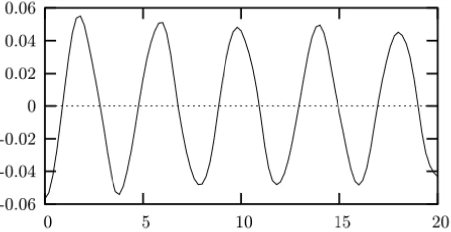
andT = 3. Fig. 1 and Fig. 2, respectively, shows the temperatureθ (x,t)and the displacementu(x,t)in the midpointx =0.
20 15
10 5
0 0.04
0.03
0.02
0.01
0
-0.01
Figure 1 – Temperature at midpointθ (0,t).
20 15
10 5
0 0.06
0.04
0.02
0
-0.02
-0.04
-0.06
Figure 2 – Displacement at midpointu(0,t).
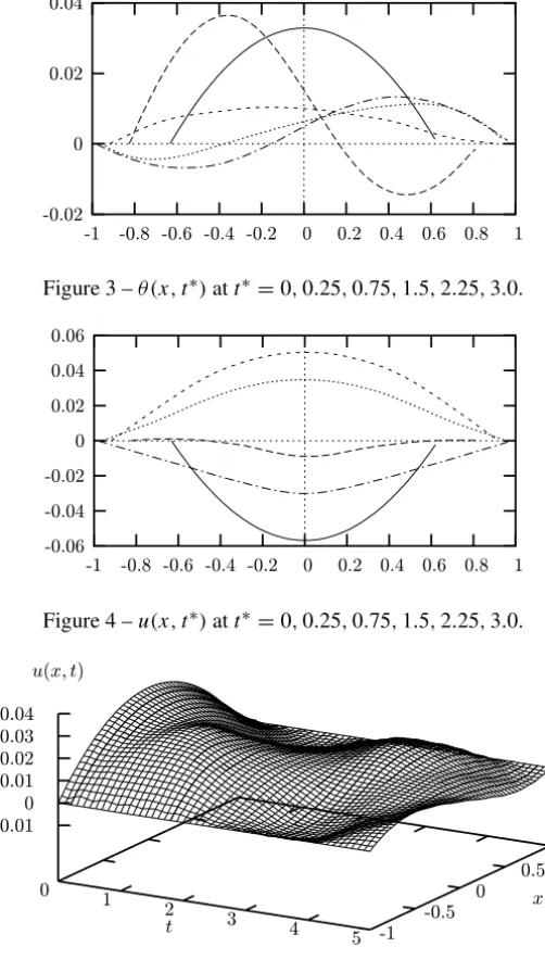
Fig. 3 and Fig. 4, show the approximate solutionsθ (x,t∗)andu(x,t∗), in the in-terval[0,T] = [0,3]for different values oft∗,t∗=0,0.25,0.75,1.5,2.25,3.0. Note that the interval of the boundary has varied from [−0.63, 0.63] to [−0.98, 0.98].
1 0.8 0.6 0.4 0.2 0 -0.2 -0.4 -0.6 -0.8 -1 0.04
0.02
0
-0.02
Figure 3 –θ (x,t∗)att∗=0,0.25,0.75,1.5,2.25,3.0.
1 0.8 0.6 0.4 0.2 0 -0.2 -0.4 -0.6 -0.8 -1 0.06
0.04
0.02
0
-0.02
-0.04
-0.06
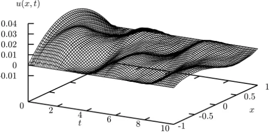
Figure 4 –u(x,t∗)att∗=0,0.25,0.75,1.5,2.25,3.0. u(x, t)
0.04 0.03 0.02 0.01 0 -0.01
x
1 0.5 0 -0.5 -1
t
5 4 3 2 1 0
Figure 5 – Displacement with 50 time steps.
u(x, t)
0.04 0.03 0.02 0.01 0 -0.01
x
1 0.5 0 -0.5 -1
t
10 8 6 4 2 0
Figure 6 – Displacement with 100 time steps.
θ(x, t)
0.06 0.03 0 -0.03 -0.06
x
1 0.5 0 -0.5 -1
t
5 4 3 2 1 0
Figure 7 – Temperature with 50 time steps.
θ(x, t)
0.06 0.03 0 -0.03 -0.06
x
1 0.5 0 -0.5 -1
t
10 8 6 4 2 0
REFERENCES
[1] S.I. Chou and C.C. Wang, Estimates of error in finite element approximate solutions to problems in linear thermoelsticity, Part II. Computationally uncoupled numerical schemes, Arch. Rational Mech. Anal.,77(1981), 263–299.
[2] J. Clank,The Mathematics of Diffusion, 2rd ed., Oxford University Press (1975).
[3] H.R. Clark, M.A. Rincon and R.D. Rodrigues,Beam Equation with Weak-Internal Damping in Domain with Moving Boundary, Applied Numerical Mathematics, Vol.47, Fasc. 2, (2003),
139–157.
[4] C.M. Dafermos,On the existence and the asymptotic stability of solution to the equations of linear thermoelasticity, Arch. Rational Mech. Anal.,29(1968), 241–271.
[5] G. Dassios and M. Grillakis,Dissipation rates and partition of energy in thermoelasticity, Arch. Rational Mech. Anal.,87-1(1984), 49–91.
[6] G.H. Golub and C.F Van Loan,Matrix Computations, 3 rd ed., Johns Hopkins U. Press, Bltimore, (1996).
[7] T.J.R. Hugles,The finite Element Method Linear Static and Dynamic Finite Element Analysis, Prentice Hall (1987).
[8] Liu, I-Shih and M.A. Rincon,Effect of Moving Boundaries on the Vibrating Elastic String, Applied Numerical Mathematics, Vol.47, Fasc. 2, (2003), 159–172.
[9] Lloyd N. Trefethen and David Bau III,Numerical Linear Algebra, 1 rd ed., SIAM, Philadelphia, (1997)
[10] L.A. Medeiros, J. Límaco and S.B. Menezes,Vibrations of Elastic Strings: Mathematical Aspects, Part One, Journal of Computational Analysis and Applications, vol.4(2002),
91–127.
[11] L.A. Medeiros, J. Límaco and S.B. Menezes,Vibrations of Elastic Strings: Mathematical Aspects, Part two, Journal of Computational Analysis and applications, vol.4(2002), 211– 263.
[12] C.A. de Moura,A linear uncoupling numerical scheme for the nonlinear coupled thermoe-lastodynamics equations, Numerical Methods, V. Pereyra and A. Reinoza (eds.). Lecture Notes in Mathematics n. 1005, Springer-Verlag, 1983.