www.elsevier.com/locate/sigpro
A new symmetric fractional B-spline
Manuel Duarte Ortigueira
∗;1UNINOVA/DEE, Faculdade de Ciˆencias e Tecnologia da UNL Campus da FCT da UNL, Quinta da Torre, Caparica 2829-516, Portugal
Received 1 December 2002
Abstract
A new denition of a symmetric fractional B-spline is presented. This generalises the usual integer order B-spline, that becomes a special case of the new one.
?2003 Elsevier B.V. All rights reserved.
Keywords:B-spline; Fractional dierintegration
1. Introduction
The signal processing with splines have been acquiring increasing interest due to its exibility in interpola-tion, sampling and wavelet transform [3]. Recently, causal and symmetric fractional B-splines were proposed [4]. We have nothing to say relatively to the proposed causal splines. In fact they generalise the integer order B-splines in such a way that these are special cases of the fractional. However, this does not happen with the fractional ones. A closed look into the proposed B-spline denitions reveals that they are strange since the even integer order B-splines are not special cases of the fractional B-spline. Here, we will face the problem and propose new denitions that have the current integer order B-splines as particular cases.
2. Causal B-splines
Causal B-splines result from n-fold convolution of the rectangle function
0+(t) =
1 0¡ t ¡1
1
2 t= 0;1
0 t ¡0 or t ¿1:
(1)
∗Tel.: +21-294-8520; fax: +21-295-7786.
E-mail address:[email protected](M.D. Ortigueira).
1Also with INESC, R. Alves Redol, 9, 1000-029 Lisboa, Portugal.
0165-1684/$ - see front matter?2003 Elsevier B.V. All rights reserved.
Its Laplace transform (LT) is an analytical function given by
Bn+(s) =
1−e−s
s n+1
(2)
that can be expressed as
Bn+(s) = 1 sn+1
n+1
k=0
n+ 1
k (−1)
ke−sk for Re(s)¿0: (3)
As
LT−1[s−n−1] = t
n
n!u(t) = tn
+
n! (4)
we obtain, from (3):
n+(t) = 1
n! n+1
k=0
n+ 1
k (−1)
k(t−k)n
+: (5)
The situation is slightly dierent when we try to dene a fractional spline. In this (causal) case, there is no problem. We only have to substitute for n in (3) and (5) and summing up to ∞:
+(t) = 1
(+ 1) +∞
k=0
+ 1
k (−1)
k(t−k)
+ (6)
It is important to remark that, while (3) represents a symmetric (relatively ton=2), for every positive integer, this does not happen with (6). This has implications in dening a symmetric fractional B-spline. The previous results are equal to those obtained in [4].
3. Symmetric B-splines
A nth degree B-spline, 0n(t), is a symmetric function resulting from n-fold convolution of the rectangle function
00(t) =
1 |t|¡12
1 2 |t|=
1 2
0 |t|¿12:
(7)
Its bilateral Laplace transform (BLT) is an analytic function given by
Bn0(s) =
es=2−e−s=2
s
n+1 =e
s(n+1)=2
sn+1
n+1
k=0
n+ 1
k (−1)
ke−sk: (8)
So, the corresponding FT exists and is given by
Bn0(!) =
sin(!=2) !=2
n+1 =e
j!(n+1)=2
(j!)n+1
n+1
k=0
n+ 1
k (−1)
From (8), we obtain:
n0(t) = 1
n! n+1
k=0
n+ 1
k (−1)
k
t−k+n+ 1 2
n
+
: (10)
On the other hand, introducingtn0=tnsgn(t)
FT−1[(j!)−n−1] =1 2
tnsgn(t)
n! = tn
0
2n! (11)
we obtain, from (9):
n0(t) = 1 2:n!
n+1
k=0
n+ 1
k (−1)
k
t−k+n+ 1 2
n
0
(12)
that seem to be dierent from (10), but due to the symmetry of the coecients it represents the same function. In [4], a symmetric fractional B-spline is dened as inverse FT of the function:
B0(!) =
sin(!=2)
!=2
+1
: (13)
However, this denition has the disadvantage of giving a strange spline, when is an even positive integer. To avoid this, we are going to present a centred fractional spline that does not have this drawback. Let=n+, wheren is a positive integer and 0¡ ¡1. We dene a fractional -order B-spline as the function that has
B0(!) =
sin(!=2)
!=2
n+1
sin(!=2) !=2
(14)
as FT. When is an integer, = 0 and we obtain the normal n-order B-spline, while when = 0, we obtain a fractional centred and symmetric B-spline that is the convolution of two even functions. The reason of proposing such denition in the fact that the inverse FT of [sin(!=2)=!=2] is a complex function.
For computing0+n(t), we can proceed recursively by successive convolutions with 0 0(t).
0+n(t) =0+n−1(t)∗00(t) (15)
From (15) and noting that 0
0(t) =u(t+12)−u(t− 1
2) we obtain:
0(t) =
t+12
t−1 2
0−1() d (16)
and
d
0(t)
dt =
−1
0 (t+12)−
−1
0 (t−12): (17)
On the other hand, if 1=n+ and2=m+, with + ¡1,
1 0 (t)∗
2 0 (t) =
1+2+1
0 (t): (18)
As shown in Appendix A, we have:
|2 sin(!=2)|[2 sin(!=2)]n+1=e j!(n+1)=2
(j)n+1 +∞
k=−∞
a(n; k) e−j!k (19)
with
a(n; k) = (+n+ 2) (=2 + 1)(=2 +n+ 2)
1 k= 0
−
=2−n−1 =2 + 1
k
k ¿0
−=2 =2 +n+ 2
|k|
k ¡0
: (20)
We are in conditions to express (14) in the Fourier series format:
B0(!) = 1 |!|(j!)n+1
+∞
k=−∞
a(n; k) e−j!(k−(n+1)=2): (21)
The inverse Fourier transform of 1=|!|(j!)n+1 is computed in Appendix B and is given by
FT−1
1 |!|(j!)n+1
= 1
2(+n+ 1)cos(=2)|t|
+nsgnn+1(t): (22)
Inserting (22) into (21) and using (20) we obtain:
0+n(t) = (+n+ 1)
2 cos(=2)(=2 + 1)(=2 +n+ 2) +∞
k=−∞
b(n; k)
t−k+n+ 1 2
+n
×sgnn+1
t−k+n+ 1 2
(23)
that is the expression of the =+n order B-spline. The coecients b(n; k) are given by
b(n; k) =
1 k= 0
−
=2−n−1 =2 + 1
k
k ¿0
−=2 =2 +n+ 2
|k|
k ¡0
(24)
that have a form suitable for recursive computation.
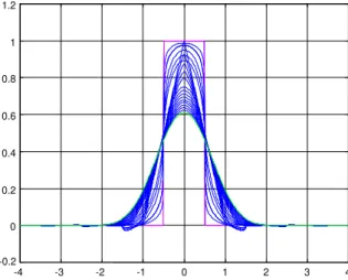
In Figs. 1–4 we present some splines for values of n= 0; 1;2; and 3 and = 0:2; 0:4;0:6;0:8, and 0.9.
To make a fair comparison, in Fig. 5, we present in the same time scale all the order splines with
-3 -2 -1 0 1 2 3 -0.2
0 0.2 0.4 0.6 0.8 1 1.2
-4 -3 -2 -1 0 1 2 3 4 -0.2
0 0.2 0.4 0.6 0.8 1 1.2
Fig. 1. Splines of orders 0, 0.2, 0.4, 0.6, and 0.8. Fig. 2. Splines of orders 1, 1.2, 1.4, 1.6, and 1.8.
-5 -4 -3 -2 -1 0 1 2 3 4 5 -0.1
0 0.1 0.2 0.3 0.4 0.5 0.6 0.7 0.8
-6 -4 -2 0 2 4 6 -0.1
0 0.1 0.2 0.3 0.4 0.5 0.6 0.7
Fig. 3. Splines of orders 2, 2.2, 2.4, 2.6, and 2.8. Fig. 4. Splines of orders 3, 3.2, 3.4, 3.6, and 3.8.
4. Conclusions
In this paper we proposed a new fractional order B-spline generalising the usual integer order B-spline that is a special case of the new one. Examples illustrate this fact and show that the fractional order interpolate the integer ones. The main drawback is in the discontinuity relatively to the order when we approach each integer from the left.
Appendix A. The Fourier series of|2 sin(!=2)|
[2 sin(!=2)]n+1
We begin by noting that
|2 sin(!=2)|= lim s→j![1−e
-4 -3 -2 -1 0 1 2 3 4 -0.2
0 0.2 0.4 0.6 0.8 1 1.2
Fig. 5. Splines of ordersn+withn= 0;1;2;3 and= 0;0:2;0:4;0:6 and 0.8.
Expanding each term on the right using the binomial series and computing the autocorrelation of the coecients we obtain the Fourier series associated to the function on the left. To do it we remark that for every ∈R, but non-even integer [1].
∞
k=0
k
k+n =
(1 + 2)
(+n+ 1)(−n+ 1) (A.2)
leading to
|2 sin(!=2)|=(+ 1)
+∞
k=−∞
(−1)k
(=2 +k+ 1)(=2−k+ 1)e
−j!k: (A.3)
On the other hand,
[2 sin(!=2)]n+1=e
j!(n+1)=2
(j)n+1
n+1
k=0
n+ 1
k (−1)
ke−j!k: (A.4)
The product of (A.3) and (A.4) has the Fourier series:
|2 sin(!=2)|[2 sin(!=2)]n+1=ej!(n+1)=2 (j)n+1
+∞
k=−∞
a(n; k) e−j!k (A.5)
with
a(n; k) =(+ 1)(−1)k n+1
m=0
n+ 1
m
(=2 +k−m+ 1)(=2−k+m+ 1): (A.6)
It is not hard to show that (A.6) can be written in terms of the Gauss hypergeometric function:
a(n; k) =(+ 1) (−1) k
(=2 +k+ 1)(=2−k+ 1) n+1
m=0
=(+ 1) (−1)
k
(=2 +k+ 1)(=2−k+ 1)2F1(−n−1;−=2−k;=2−k+ 1; 1): (A.7)
Using the properties of the hypergeometric function, we obtain:
a(n; k) = (−1)k (+n+ 2)
(=2 +k+ 1)(=2−k+n+ 2)= (−1)
k
+n+ 1
=2 +k : (A.8)
Letting q(n+ 1; k) be given by
q(n; k) = (−1)
k
(=2 +k+ 1)(=2−k+n+ 2) (A.9)
we can express it as
q(n; k) = 1
(=2 + 1)(=2 +n+ 2)
1 k= 0
−
=2−n−1 =2 + 1
k
k ¿0
−=2 =2 +n+ 2
|k|
k ¡0
(A.10)
where we represented (a)k=(b)k by [a=b]k for simplication. Thus,a(n; k) is given by
a(n; k) = (+n+ 2) (=2 + 1)(=2 +n+ 2)
1 k= 0
−=2−n−1 =2 + 1
k
k ¿0
−
=2 =2 +n+ 2
|k|
k ¡0
: (A.11)
It is interesting to remark that, if= 0; a(n; k) = 0 for k ¡0 anda(n; k) = (−1)kn+1
m
for k= 0;1; : : : ; n+ 1, leading to (12).
Appendix B. Inverse transform of|!|−( j!)−n−1
To compute the inverse Fourier transform ofG(!) =|!|−(j!)−n−1 we write it as
G(!) =|!|−(j!)−n−1
= (−j) n+1
|!|+n+1
1 ! ¿0
(−1)n+1 ! ¡0: (B.1)
If n is odd, we obtain:
G(!) =(−1)
n+1=2
|!|+n+1 : (B.2)
while, if n is even,
G(!) =(−j)(−1)
n=2
If is a noninteger real, the inverse Fourier transform of |!|− is given by [2]:
FT−1[|!|−] =(1−)sin(=2)
|t|
−1 (B.4)
or
FT−1[|!|−] = 1
2()cos(=2)|t|
−1: (B.5)
We obtain immediately to (B.2):
FT−1[G(!)] = 1
2(+n+ 1)cos(=2)|t|
+n: (B.6)
To treat the n even case, we only have to remark that
1
|!|+n+1sgn(!) =−
d d!
1 (+n)|!|+n
and use the property: FT[t f(t)] = jF′(!). We obtain, then:
FT−1[G(!)] = 1
2(+n+ 1)cos(=2)t|t|
+n−1= 1
2(+n+ 1)cos(=2)|t|
+nsgn(t): (B.7)
We can join (B.5) and (B.6) in the form:
FT−1
1 |!|( j!)n+1
= 1
2(+n+ 1)cos(=2)|t|
+nsgnn+1(t) (B.8)
or
FT−1
1
|!|(j!)n+1
= 1
2(+n+ 1)cos(=2)|t|
tnsgn(t) (B.9)
that gives (11) when = 0.
References
[1] M.D. Ortigueira, Introduction to fractional signal processing, Part 2: Discrete-time systems, IEE Proceedings on Vision, Image and Signal Processing, Vol. 1, February 2000, pp. 71–78.
[2] S.G. Samko, A.A. Kilbas, O.I. Marichev, Fractional Integrals and Derivatives—Theory and Applications, Gordon and Breach Science Publishers, London, 1987.