Numerical modeling of contact problems with the finite element
method utilizing a B-Spline surface for contact surface smoothing
Abstract
The basic aim of this work is to present a method to treat structural mechanics problems dealing with tridimensional contact and large elastic deformations. The formulation presented in this article offers a B-Spline based discretization for the contact surface, which solves the continuity problems presented by the classic Lagrangian contact element formulation. A Spline surface is utilized to discretize the contact surface, and the B-Spline basis functions are used to distribute the contact forces between the contact surfaces nodes. The finite element utilized is an 8-node hexahedron, and the formulation is continuum mechanics based, written in the current configuration, utilizing a neo-Hookean material model. The contact restrictions are enforced by the augmented Lagrangian method.
Key-words
Contact mechanics, B-Spline, Surface smoothing, Augmented Lagrangian method, Friction.
1 INTRODUCTION
Finite element contact simulations exhibiting large deformations has been growing as a subject of study in the last few decades. Many works have been produced about it, and one can cite WRIGGERS in 1989 and 1996, BENSON (1990) and LAURSEN AND SIMO in 1993 as authors giving important contributions to the field, as well as CURNIER in 1999, and BANDEIRA in 2001, who offered further research on the subject.
The classical way to discretize a contact surface on a tridimensional problem is through the Lagrangian contact element. The Lagrangian contact element for a hexahedron finite element mesh is a 4-node, linear element, which results in a flat surface. When discretizing a curved surface, the Lagrangian contact element, being a linear element, leads to a facetization of the contact surface, i. e., the curved surface is represented by several flat surfaces, side by side, with an angle between them. This facetization leads to a geometric discontinuity of the contact surface, and therefore, generates discontinuity of the normal vector. This in turn, leads to convergence problems, especially when large sliding occurs.
To tackle this issue, many approaches have been proposed. One may consider, between many options, the Mortar method, described in (PUSO, LAURSEN and SOLBERG, 2008), the Hermitian element (WRIGGERS, 2006) and (ALAIN BATAILLY, 2013), the smoothing of the contact surface using B-Splines or NURBS surfaces (CALLUM and CORBETT, 2014), a combination of NURBS and Mortar presented by (TEMIZER, 2011), or the isogeometric analysis as proposed by (M.E. MATZEN, 2012) and (DE LORENZIS, WRIGGERS, ZAVARISE, 2012), which does away with the classical Lagrangian element, and utilizes a new contact element based on B-Spline or NURBS basis function.
This paper describes an isogeometric approach, where a B-Spline patch is used to discretize a contact surface over the master body. The difference between this paper and other works which utilize the isogeometric approach is that no smoothing of the slave surface is done. The smoothing is done only on the master surfaces.
Daniel Barbedo Vasconcelos Santosa*
Alex Alves Bandeira b
a Programa de pós-graduação em engenharia de estruturas, Departamento de construção e estruturas, Universidade Federal da Bahia - UFBA, Salvador, Bahia, Brasil. E-mail: [email protected]
b Departamento de construção e estruturas, Universidade Federal da Bahia - UFBA, Salvador, Bahia, Brasil.
E-mail: [email protected]
*Corresponding author
http://dx.doi.org/10.1590/1679-78254891
authors believe that when contact happens, the slave surface will assume the master surface’s shape, and thus will also be smoothed.
In the first section of this article, a brief description of the contact problem, the virtual work applied to the balance of linear momentum equation and the Neo-Hookean material constitutive equation are presented. Then, the equation for contact forces is shown. Afterwards, the B-Spline concept is briefly described, and the method for discretizing the contact surface using the B-Spline is detailed. The relevant equations for the contact pressures, their linearization and finally the relevant vectors for the discretization of the contact surfaces are presented.
In the last section numerical examples are shown, utilizing the formulation presented in this paper. The results obtained are compared to the commercial software ANSYS and afterwards the results are briefly discussed.
2 PROBLEM DESCRIPTION
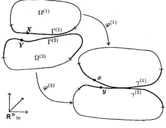
It is shown, in Figure 1, a tridimensional contact problem between two deformable solids as described in (SIMO, LAURSEN, 1992). The group of material points, that belong to the bodies in the reference position, are called B and B . Additional configurations can be obtained by the transformations φ : B × I → R and φ : B × I → R in the interval t = [0, T]. The bodies B and B , subject to contact, are called slave and master. In each of these bodies, there is a boundary where contact can be expected. These boundaries are called Г and Г . Г is the slave boundary, belonging to the body B , and Г the master boundary, belonging to the body B . These boundaries are in the reference configuration, and are subject to the same transformations φ and φ that the bodies B and B are subject. A point belonging to body B is denoted by X in the reference configuration and x on the current configuration, and the same applies for body B , exchanging the index.
Figure 1:Notation for the contact problema with friction
The displacement u is defined as, 𝐮 = 𝐱 − 𝐗 = φ(𝐗 , t) − 𝐗 , (2.1) with α = 1,2.
|g(𝐗, t)| = min ∈Г |φ (𝐗 , t) − φ (𝐗 , t)| . (2.2)
The minimum for this function can be calculated by finding the roots of the first derivate.
3 VIRTUAL WORK PRINCIPLE
The equilibrium equation, derived from the balance of linear momentum is defined by, Div 𝐏( )+ ρ 𝐛̅ − ρ 𝐯= 0, (3.1)
where 𝐏 is the first Piola Kirchoff tensor, ρ is the body’s density and 𝐛̅ the body forces for unit of volume.
After applying virtual displacements, and bringing the tensors from the reference configuration to the current configuration, one obtains
w(φ, η) = ∫( )𝛔 ∙ ∇ 𝛈dV − ∫ ( )ρ 𝐛 − 𝐯 ∙ 𝛈dV − ∫ ( )𝐭 ∙ 𝛈dA = 0. (3.2)
In this equation, 𝛔 is Cauchy’s tensor and ρt is density for current unit of volume. This equation represents equilibrium between the internal work and the external work defined at the current configuration.
It’s necessary to include the material behavior in the finite element simulation, thus an equation for a material model is necessary. The Neo-Hookean material model is adopted on this article. This material model is adequate for simulating large tridimensional displacements. Therefore, Cauchy’s tensor on the equation (3.2) is obtained through the deformation energy function for a Neo-Hookean material, given by
𝛔 = (J − 1)𝐈 + (𝐛 − 𝐈). (3.3)
Equation (3.2) can be divided into two parts, internal and external forces. The first term represents the internal forces, and the second and third terms represent the external forces,
П = ∫( )𝛔 ∙ ∇ 𝛈dV (3.4) and
П = ∫ ( )ρ 𝐛 − 𝐯 ∙ 𝛈dV − ∫ ( )𝐭 ∙ 𝛈dA. (3.5)
Moreover, since the problem being simulated is a contact problem, the equations need to depict the behavior of both bodies, , as exhibited on (LAURSEN, 2002). Equation (3.2) is then expanded to include both bodies, W(φ, η) = ∑ ∫ (𝛔 ∙ ∇ 𝛈dV )𝛂
( ) − ∫ ρ 𝐛 −
𝐯
∙ 𝛈dV − ∫ ( ) 𝐭 ∙ 𝛈dA
( ) = 0. (3.6)
To satisfy the impenetrability condition and to represent the contact forces, a contact energy term is added to equation (3.6).
П + П + П = 0 (3.7)
The definition of П depends upon the restriction method utilized. In this paper, the augmented Lagrangian method was utilized, as described in (BANDEIRA, et al., 2010), (BERTSEKAS, 1995) and (LUENBERGER, 1984).The contact equation is defined, as shown in (BANDEIRA, 2001), (WRIGGERS, 2008) and (LAURSEN and SIMO, 1993a), by
П = ∫ t δg dA + ∫ 𝐭 δ𝐠 dA. (3.8)
The terms t and 𝐭 represent the normal and tangencial contact pressures, respectively. g represents the gap function, which notates the penetration between the bodies, and 𝐠 is the tangencial displacement function, which represents how much one of the bodies slides over the other.
Equation (3.7) then can be discretized and solved by the finite element method. In this paper, the isoparametric hexahedral element was used. More details on the finite element discretization can be found on (BATHE, 1996), (ZIENKIEWICZ, TAYLOR, ZHU, 2005), and (COOK, 2002).
4 NODE TO SURFACE FORMULATION
In this section, the node-to-surface contact formulation is expressed, for more details, refer to (WRIGGERS, 2008) and (BANDEIRA, 2001). The contact formulation is independent of the finite element utilized for its discretization, hence it can be used for a B-Spline based finite element.
The equation for the contact forces as found in BANDEIRA is defined in (3.8) and is repeated here for convenience,
C = ∫ t δg dA + ∫ 𝐭 δ𝐠 dA. (4.1)
The first term accounts for the normal forces and the second one to the tangential forces. When the augmented Lagrangian method is used to enforce the contact restriction, the term t is defined by
t =< λ + ξ g >, (4.2)
where λ is the Lagrangian multiplier, ξ is the penalty factor and g is the gap function. In turn, g which is defined by
g = (𝐱 − 𝐱 ) ∙ 𝐧 if (𝐱 − 𝐱 ) ≤ 0 0 if (𝐱 − 𝐱 ) > 0 , (4.3)
where 𝐱 is the point of the slave surface currently analyzed, or rather, a node, and 𝐱 is the projection of the slave point on the master surface.
The term δg is given by δg = (𝐯 − 𝐯 ) ∙ 𝐧 . (4.4)
The second term of equation (4.1) accounts for the friction forces, parallel to the contact surface. On that equation, 𝐭 depends on the friction model utilized. In this paper, the Coulomb friction model was deemed sufficient. In the Coulomb friction model, the term 𝐭 depends on whether the friction is on the stick case, where the two bodies don’t move relative to each other, or the slip case, where one body slides over the other. Depending on which is the current case, 𝐭 is calculated differently. The following functions are used to calculate it.
t = 𝐭 ⋅ 𝐚 (4.5) and
t =
t se Φ ≤ 0
μ 𝐭 se Φ > 0 (4.6)
The value of Φ defines whether the current node is on a stick or slip case, and then t is defined accordingly. t is defined by
t = t + ∆λ + ξ u , (4.7) and Φ is given by
ϕ = [t m( )t ]/ − μ t . (4.8)
For more details regarding the node-to-surface formulation utilizing the augmented Lagrangian method to enforce contact restrictions, one can refer to (BANDEIRA, 2001).
with ξ̅̇ defined by
ξ̅̇ = [𝐯 − 𝐯 ] ∙ 𝐚 + g 𝐧 𝐯, (4.10)
and the following terms defined as follows, a = 𝐱, ξ̅ ∙ 𝐱, ξ̅ = a ∙ a , (4.11) b = 𝐱, ξ̅ ∙ 𝐧 = 𝐱, ∙ 𝐧 , (4.12) and
𝐚 = 𝐱 ( , )= 𝐱, (ξ , t). (4.13)
4.1 Linearization
The solution for the equation (4.1) is discovered using Newton-Raphson’s method, and as such, the derivatives of equation (4.1) are necessary. The derivative is given by
K = ∫ [∆t δg + t ∆(δg )]dA + ∫ ∆t δξ̅ + t ∆ δξ̅ dA. (4.14)
For the first integral, the term ∆t is given by ∆t = ε ∆g , (4.15)
with ∆g defined as
∆g = (∆u − ∆u ) ⋅ n , se g < 0 0, se g > 0 , (4.16)
and t and δg as shown previously. The term ∆(δg ) is given by
∆(δg ) = −𝐯, ∆ξ̅ ⋅ 𝐧 − (𝐯 − 𝐯 ) ⋅ 𝐚 a 𝐧 ⋅ ∆𝐮, + 𝐚 , ∆ξ̅ , (4.17) where ∆ξ̅ is defined by
∆ξ = [∆𝐮 − ∆𝐮 ] ⋅ 𝐚 + g 𝐧 ⋅ 𝐮, . (4.18)
In the second term of equation (4.14), ∆t is defined as ∆t = ∆t = ϵ ∆ξ̅ 𝐚 + ϵ ξ̅ − ξ̅ ∆a (4.19)
for the stick case, with ∆a given by ∆a = ∆𝐚 ∙ 𝐚 + 𝐚 ∙ ∆𝐚 . (4.20)
For the slip case, ∆t is defined as
∆t = μϵ ∆g 𝐭 + μ 𝐭 ∆t + μ
𝐭 t t (𝐭 ∆𝐚 − ∆t ), (4.21)
with ∆t being given by
∆t = ϵ a ∆ξ + ϵ ξ̅ − ξ̅ (∆𝐮, + 𝐚 , ∆ξ̅ ∙ 𝐚 + 𝐚 ∙ (∆𝐮, + 𝐚 , ∆ξ̅ )}. (4.22)
Following that, δξ̅ is defined as
δξ = [𝐯 − 𝐯 ] ⋅ 𝐚 + g 𝐧 ⋅ 𝐯, , (4.23)
∆ δξ̅ = {−𝐚 ⋅ v, ∆ξ̅ + ∆u, δξ̅ + 𝐚 , δξ̅ ∆ξ̅ + ∆u, + a , ∆ξ̅ ⋅ 𝐯 − 𝐯 − 𝐚 δξ̅ + v, + 𝐚 , δξ̅ ⋅ ∆𝐮 − ∆𝐮 − 𝐚 ∆ξ̅ + g n ⋅ v, ∆ξ̅ + ∆u, δξ̅ + 𝐚 , δξ̅ ∆ξ̅ . (4.24)
5 CONTACT ELEMENT DISCRETIZATION
The solids bodies involved in the contact problem must be discretized into a finite element mesh. In this paper, the bodies are discretized by 8-node hexahedron elements, and the contact surface is discretized using a B-Spline based finite element.
Using a B-Spline based finite element for the discretization of the contact surfaces gives a few advantages over the Lagrangian 4-node contact element, such as a smooth surface and a higher degree of continuity between elements, avoiding the numerical problems associated with the node-surface formulation. The definition for B-Spline surfaces is briefly shown in the next session, and it’s followed by the procedure to discretize the contact surface using a B-Spline based finite element.
5.1 B-Spline surface
A B-Spline surface is constructed based on the interpolation of a number of spatial points. These points are called control points, and their spatial coordinates are interpolated using a number of functions called base functions to construct a tridimensional surface.
The B-Spline parametric surface is constructed using the base functions. In turn, the base functions are built based on a parameterization of space given by the knot vectors, i. e.
Ξ = [ξ , ξ , ξ … ξ ]. (5.1)
𝜉 represents the knots. The knots define the limits of the base functions domain, by dividing the parametric space into discrete elements. The knot vector has 𝑛 elements, 𝑛 being the sum of the number of control points plus the order k of the base function. The order of the base function represents the number of intervals between knots that composes the function’s domain. An open knot vector has its first and last entries repeated k times. The open knot vector makes the curve or surface to behave the same when close to its borders as it behaves in the middle.
A point in the B-Spline surface is given by 𝐐(t, u) = ∑ ∑ 𝐁,N, (ξ)M,(η), (5.2)
where 𝐁 is a control point, N and M are the base functions, one increasing in a different direction to the other. k and l are the order of the base functions. The B-Spline base function is given by
N, (ξ) = 1 se x ≤ ξ < x0 caso contrário N, (ξ) =( ) , ( )+( ) , ( ). (5.3)
The base functions are built recursively, with higher orders needing more calculations and thus processing power on a numerical analysis. An order of 1 reduces the base function to a Lagrangian base function.
B-Spline surfaces enjoy 𝐶 continuity, where k is the order of the base function, and m is the multiplicity of an inner knot i. In this paper, other than an open knot vector, no knot vector manipulation was used, so the multiplicity of any inner knot is 1.
More detailed information about B-Spline and NURBS curves can be found on (LES PIEGL, 1997) and (ROGERS, 2001).
5.2 B-Spline based finite elements
When the classic Lagrangian 4-node contact element is used, multiple contact elements are utilized to form a contact surface. When there’s contact between a slave node and the master surface, the resulting contact forces are distributed between the slave node, and the four nodes belonging to the single contact element where contact was detected.
On this paper, B-Spline based isogeometric analysis is utilized. A single B-Spline surface, or patch, is utilized to represent the whole contact surface on the master body. As such, a B-Spline surface is constructed using the nodes of the master’s surface contact area.
More details about isogeometric analysis can be found on (AUSTIN COTTRELL, 2009) and a bi-dimensional isogeometric analysis can be seen on (DE LORENZIS, 2011).
distribution. As a general rule, the further away from the contact point the node is, smaller is the contact force acting on that node.
For the numerical examples executed, the methodology found in (BANDEIRA, 2001) was followed, but utilizing a B-Spline based finite element surface in place of a Lagrangian element contact surface mesh. As such, only the master surface is discretized with the B-Spline finite elements, the slave surface is not discretized, but each of its nodes is checked for contact against the master surface.
The knot vectors used to construct the B-Spline surface patch are constructed dynamically, based on the number of nodes taken as control points in the appropriate direction.
6 DISCRETIZATION OF CONTACT FORCES
Discretization of the contact work described in equation (4.1) can be written in vector form as W (𝐮, 𝐯) = ∑ A 𝐑 ⋅ 𝐕 , (6.1)
where A represents the contact finite element area, ns is the total number of slave nodes, 𝐕 represents the derivative of the spatial position of the element nodes and 𝐑 represents the contact stresses.
Expressing this in a vector representation 𝐑 = t 𝐍 + t 𝐃 = t 𝐍 + t 𝐃 + t 𝐃 (6.2) with the vectors being defined by
𝐕 = ⎣ ⎢ ⎢ ⎢ ⎢ ⎢ ⎢ ⎢ ⎢ ⎡ 𝐯𝐯
𝐯 𝐯 … 𝐯 𝐯
𝐯 ⎦⎥ ⎥ ⎥ ⎥ ⎥ ⎥ ⎥ ⎥ ⎤ 𝐍 = ⎣ ⎢ ⎢ ⎢ ⎢ ⎢ ⎢ ⎢ ⎢ ⎢ ⎡ −Q 𝐧𝐧𝐜
𝐜 −Q 𝐧 −Q 𝐧 … −Q 𝐧 −Q 𝐧
−Q 𝐧 ⎦⎥ ⎥ ⎥ ⎥ ⎥ ⎥ ⎥ ⎥ ⎥ ⎤
𝐍𝛂=
⎣ ⎢ ⎢ ⎢ ⎢ ⎢ ⎢ ⎢ ⎢ ⎢ ⎢ ⎢ ⎡ −Q𝟎
, 𝐧 −Q , 𝐧 −Q , 𝐧 … −Q , 𝐧 −Q , 𝐧 −Q
, 𝐧 ⎦ ⎥ ⎥ ⎥ ⎥ ⎥ ⎥ ⎥ ⎥ ⎥ ⎥ ⎥ ⎤ 𝐓 = ⎣ ⎢ ⎢ ⎢ ⎢ ⎢ ⎢ ⎢ ⎢ ⎢ ⎡ −Q 𝐚𝐚
−Q 𝐚 −Q 𝐚 …
−Q 𝐚
−Q 𝐚
−Q 𝐚 ⎦⎥ ⎥ ⎥ ⎥ ⎥ ⎥ ⎥ ⎥ ⎥ ⎤
D =a − g b1 T − g N δξ̅ = D ∙ V
where Q / is defined as Q / = N , (t)M ,(u), (6.3)
with “a” and “b” being the index number of the control points that construct the surface patch in each direction, and “k” and “l” are the selected base function’s order, omitted for brevity.
The linearization of equation (6.1) is necessary to solve the problem for the displacements, so it’s given by
𝐮 ∆𝐮 = ∑ A (𝐕 ) 𝐊 ∆𝐔 (6.4)
with 𝐊 representing the stiffness matrix of the element.
To create the stiffness matrix contribution due to contact forces, a discretization of the equation is necessary. This discretization, in vector form, is given by
𝐊 = ϵ 𝐍𝐍 + t 𝐍 𝐃 + a 𝐓 𝐍 − 𝐃 n ⋅ a , (6.5)
∆𝐔 = ⎣ ⎢ ⎢ ⎢ ⎢ ⎢ ⎢ ⎢ ⎡ ∆𝐮∆𝐮𝐒/
∆𝐮 / ∆𝐮 / … ∆𝐮 / ∆𝐮 /
∆𝐮 / ⎦ ⎥ ⎥ ⎥ ⎥ ⎥ ⎥ ⎥ ⎤ 𝐏 = ⎣ ⎢ ⎢ ⎢ ⎢ ⎢ ⎢ ⎢ ⎢ ⎢
⎡ −Q 𝟎 / , 𝐭 −Q / , 𝐭 −Q / , 𝐭 … −Q / , 𝐭 −Q / , 𝐭
−Q / , 𝐭 ⎦⎥ ⎥ ⎥ ⎥ ⎥ ⎥ ⎥ ⎥ ⎥ ⎤ 𝐓 = ⎣ ⎢ ⎢ ⎢ ⎢ ⎢ ⎢ ⎢ ⎢ ⎡ −Q 𝟎
/ , 𝐚 −Q / , 𝐚 −Q / , 𝐚
… −Q / , 𝐚 −Q / , 𝐚
−Q / , 𝐚 ⎦⎥ ⎥ ⎥ ⎥ ⎥ ⎥ ⎥ ⎥ ⎤ 𝐓 = ⎣ ⎢ ⎢ ⎢ ⎢ ⎢ ⎢ ⎢ ⎡ −Q𝐚 ,
/ 𝐚 , −Q / 𝐚 , −Q …/ 𝐚 , −Q / 𝐚 , −Q / 𝐚 ,
−Q / 𝐚 , ⎦ ⎥ ⎥ ⎥ ⎥ ⎥ ⎥ ⎥ ⎤ 𝐍 = ⎣ ⎢ ⎢ ⎢ ⎢ ⎢ ⎢ ⎢ ⎢ ⎡ −Q 𝟎
/ , n −Q / , n −Q / , n
… −Q / , n −Q / , n −Q / , n ⎦⎥
⎥ ⎥ ⎥ ⎥ ⎥ ⎥ ⎥ ⎤ 𝐄 = ⎣ ⎢ ⎢ ⎢ ⎢ ⎢ ⎢
⎡ −Q𝟏/ 𝟏 −Q / 𝟏 −Q…/ 𝟏 −Q / 𝟏 −Q / 𝟏 −Q / 𝟏 ⎦
⎥ ⎥ ⎥ ⎥ ⎥ ⎥ ⎤ 𝐄 = ⎣ ⎢ ⎢ ⎢ ⎢ ⎢ ⎢ ⎢ ⎢ ⎡ −Q𝟎
/ , 𝟏 −Q / , 𝟏 −Q / , 𝟏
… −Q / , 𝟏 −Q / , 𝟏 −Q / , 𝟏 ⎦⎥
⎥ ⎥ ⎥ ⎥ ⎥ ⎥ ⎥ ⎤ (6.6)
7 NUMERICAL EXAMPLES
Three numerical examples were considered to test the B-Spline based finite element contact algorithm. The first one was the Parisch model (PARISCH, 1989), which was executed to compare directly with the results obtained by the Lagrangian finite element under large displacements. The second one was an authors created example, two beams subject to a significant bending moment in which both show large displacements. Finally, the third example shows two parallel beams, and it was designed to test the B-Spline finite element when the contact surface is generated after the body is significantly deformed. Lastly, the final example was designed to exhibit an amount of sliding over the contact surface.
7.1 Parisch
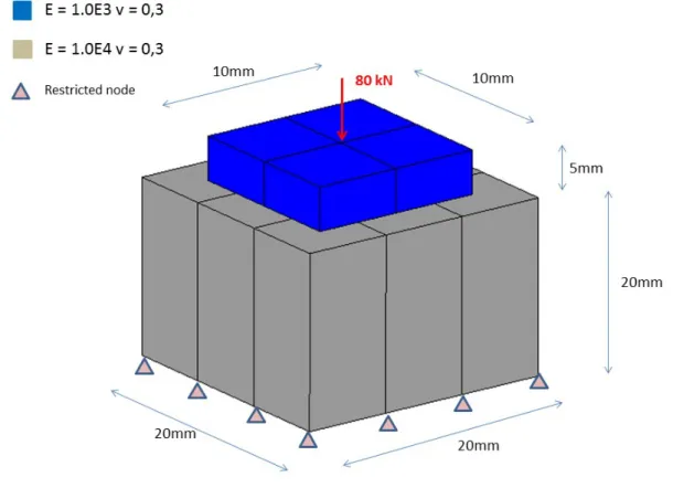
In Figure 2, one can see the example created by (PARISCH, 1989) and referenced in (BANDEIRA, 2001). It consists of two blocks, shaped like square based prisms, one supporting the other. The inferior block has all its base nodes restricted in all directions, while none of the superior block’s nodes has any restrictions. The superior block is supported only by contact forces. There are 50 nodes and 13 elements on this example, and more geometry information can be seen on Figure 2.
Figure 2: Parisch example
The resulting deformations can be observed on Figure 3. The results obtained were very close to the values obtained by Parisch. The vertical coordinate of the node where the load was applied is 21.95 on the Parisch article, and the value found on this paper was 21.94, a negligible difference.
Figure 3: Parisch displacements
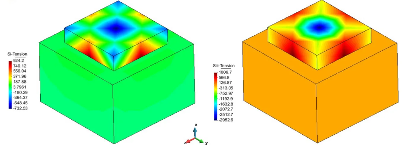
Figure 4: Parisch maximum and minimum main stresses
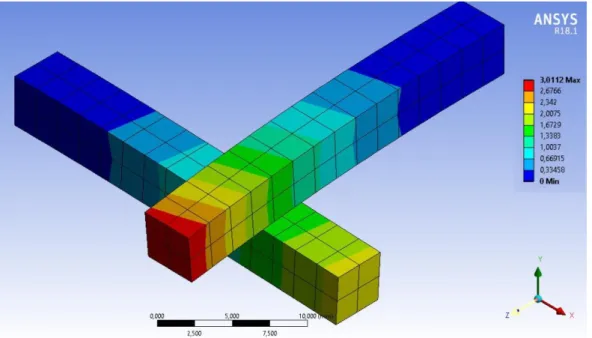
7.2 Crossed Beams
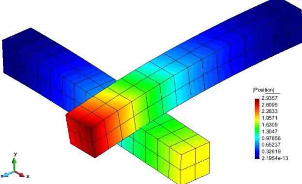
The second example can be observed on Figure 5. Created by the authors, the example consists of two beams crossed and superposed, with a 0.2 mm gap between them. On the free end of the superior beam, at the edge, a load totaling 9000N is applied. This example has 288 nodes and 120 elements. More information about the example geometry can be observed on Figure 5.
Figure 5: Crossed Beams example
This example was simulated with friction, the contact penalty parameters were ε = 10 for normal penalty and ε = 10 for the tangential penalty. The superior beam has an elasticity modulus of 4.10 Pa, while the inferior beam has 10 Pa. The friction coefficient used was μ = 0.2, and three load increments were applied.
Figure 6: Crossed Beams displacements
Figure 7: Crossed Beams displacements (lateral view)
Figure 8: Crossed Beams, ANSYS displacements
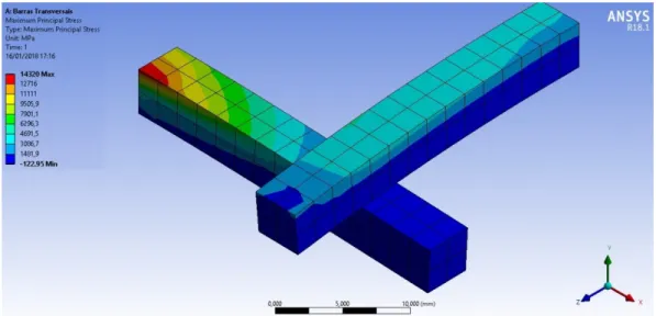
The obtained results for maximum and minimum main stresses for the crossed beams example are shown in figures 9 and 10.
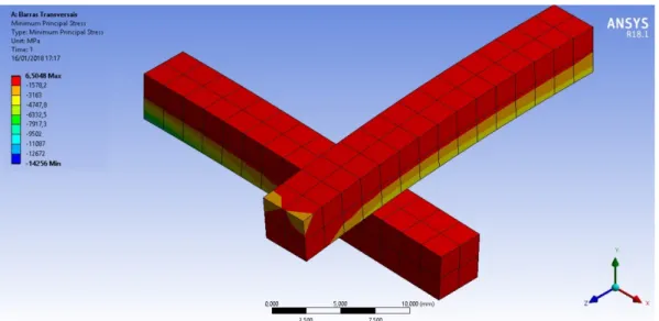
Figure 10: Crossed Beams minimum main stress
Figures 11 and 12 show the maximum and minimum stresses obtained by ANSYS.
Figure 12: Crossed Beams ANSYS minimum main stress
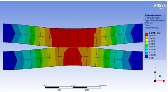
7.3 Parallel Beams
Illustrated in Figure 13, this example consists in two parallel beams, restricted on both ends, with forces applied perpendicularly. There are 384 and 180 elements in this example. The loads were applied in a way to arch the beams before contact happens, so the contact surfaces are curved.
The superior beam has double the width of the inferior one; otherwise they’re the same size. Information about restricted nodes, load positioning and details about the dimensions can be observed on Figure 8. The elasticity modulus of both beams is 10 Pa. Friction was used and the friction coefficient is μ = 0.2. 30 load increments were utilized, and the normal and tangential penalty values are ε = 10 and ε = 10 , respectively.
The deformations can be observed on Figure 14 and Figure 15.
Figure 14: Parallel Beams displacements
Figure 15: Parallel Beams displacements (frontal view)
Figure 16: Parallel Beams ANSYS displacements
Figures 17 and 18 show the maximum and minimum main stresses obtained.
Figure 17: Parallel Beams maximum main stress
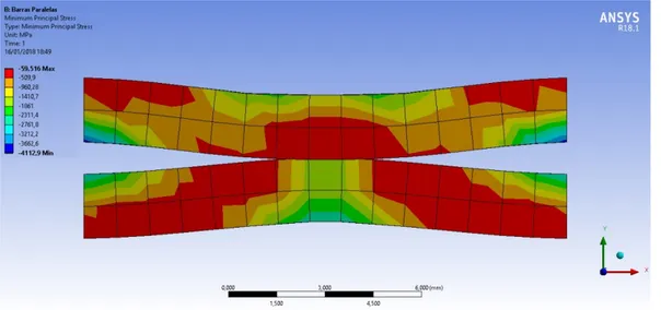
Figures 19 and 20 show the maximum and minumum main stresses obtained on ANSYS.
Figure 19: Parallel Beams ANSYS maximum main stress
Figure 20: Parallel Beams ANSYS minimum main stress
7.4 Supported Beam
Figure 21: Supported Beam example
The elasticity modulus for both beams is 10 Pa, the normal penalty utilized was ε = 5. 10 and 30 load increments were necessary for convergence.
The displacement results can be observed on Figure 22 and Figure 23.
Figure 23: Supported Beam (Isometric view)
The ANSYS results from the same mesh can be observed on Figure 24.
Figure 24: Supported Beam ANSYS displacements
Figure 25: Supported Beam maximum main stress
In figures 27 and 28, the ANSYS maximum and minimum main stresses are shown.
Figure 27: Supported Beam ANSYS maximum main stress
Figure 28: Supported Beam ANSYS minimum main stress
8 CONCLUSION
Table 1: Result comparison
Max displacement Max ANSYS
displacement (result/ANSYS results)Percentage
Crossed beams 2.9357 3.0112 97.49%
Parallel beams 0.5365 0.5488 97.76%
Supported beam 1.0972 1.1081 99.02%
The stress values found on this paper diverged from the ones found on ANSYS by a fairly significant amount. The reason for this discrepance is a difference in the Neo-Hookean energy strain equation of the material. The equation used in this paper was developed by Ciarlet-Simo, as described on (WRIGGERS, 2008),
W (I , J) = (J − 1) − ln(J) + [(I − 3) − 2 ln(J)]. (8.1)
On equation 8.1, J is the jacobian, and μ , λ are the Lamé parameters. The Neo-Hookean energy strain equation used by ANSYS, as found on its help file, is given by
W (I , J) = (J − 1) + μ (𝐛 − 𝐈), (8.2)
where b is the left Cauchy Green tensor, and K is given by K = λ + μ . (8.3)
The ANSYS stress results can still be very valuable for a qualitative comparison. One can observe that the stress distributions displayed on the results found on this paper and the ones derived from ANSYS are consistently similar.
It was shown that B-Spline based finite element and the discretization technique utilized on this paper are valid forms of smoothing the contact surface and solving the facetization problem. It provides consistent stresses across the contact surfaces and forbids penetration, especially with better discretized meshes.
The implementation of the B-Spline based finite element is relatively simple, and further studies can be done to compare performance and convergence between it and other existing smoothing techniques.
REFERENCES
ALAIN BATAILLY, B. M. N. C. A comparative study between two smoothing strategies for the simulation of contact with large sliding. Comput Mech, p. 581-601, 2013.
BANDEIRA, A. A. Análise de problemas de contato com atrito em 3D. Tese (Doutorado) - Departamento de Engenharia de Estruturas e Fundações, Escola Politécnica, Universidade de São Paulo, São Paulo, 2001. 275.
BANDEIRA, A. A. et al. Algoritmos de otimização aplicados à solução de sistemas estruturais não-lineares com restrições: uma abordagem utilizando os métodos da Penalidade e do Lagrangiano Aumentado. Exacta (São Paulo. Impresso), 8, 2010. 345-361.
BATHE, K.-J. Finite Element Procedures. First. ed. New Jersey: Prentice-Hall, Englewood Cliffs, 1996.
BERTSEKAS, D. P. Nonlinear programming. Belmont: Athena Scientific, 1995.
CALLUM J. CORBETT, R. A. S. NURBS-enriched contact finite elements. Computer methods in applied mechanics and engineering, 2014.
COOK, M. P. W. Concepts and Applications of Finite Element Analysis. 4th. ed. [S.l.]: John Wiley & Sons, INC., 2002.
DE LORENZIS, L.; WRIGGERS, P.; ZAVARISE, G. A mortar formulation for 3D large deformation contact using NURBS-based isogeometric analysis and the augmented Lagrangian method. Comput Mech, 49, 2012. 1-20.
I. TEMIZER, P. W. T. J. R. H. Contact treatment in isogeometric analysis with NURBS. Comput. Methods Appl. Mech. Engrg., p. 1100-1112, 2011.
J. AUSTIN COTTRELL, T. J. R. H. Y. B. Isogeometric Analysis. 1st. ed. [S.l.]: Wiley, 2009.
L. DE LORENZIS, I. T. P. W. G. Z. A large deformation frictional contact formulation using NURBS-based isogeometric analysis. INTERNATIONAL JOURNAL FOR NUMERICAL METHODS IN ENGINEERING, 2011.
LAURSEN, T. A. Computational Contact and Impact Mechanics. [S.l.]: Springer, 2002.
LAURSEN, T. A.; SIMO, J. C. A Continuum-Based Finite Element Formulation for the Implicit Solution of Multibody, Large Deformation Frictional Contact Problems. Int. J. Num. Meth. Engng., 36, 1993a. 3451-3485.
LES PIEGL, W. T. The NURBS Book. 2nd. ed. [S.l.]: Springer, 1997.
LUENBERGER, D. G. Linear and Nonlinear Programming. 2. ed. Reading. ed. Massachusetts: Addison-Wesley Publishing Company, 1984.
M.E. MATZEN, T. C. M. B. A point to segment contact formulation for isogeometric, NURBS based finite elements. Elselvier, 2012.
PARISCH, H. A Consistent Tangent Stiffness Matrix for Three-Dimensional Non-Linear Contact Analysis. International Journal for Numerical Methods in Engineering, 28, 1989. 1803-12.
PUSO, M. A.; LAURSEN, T. A.; SOLBERG, J. A segment-to-segment mortar contact method for quadratic elements and large deformations. Comput Methods Appl Mech Eng, 197, 2008. 555–566.
ROGERS, D. F. An Introduction to NURBS. [S.l.]: Morgan Kaufman Publishers, 2001.
SIMO, J. C.; LAURSEN, T. A. An augmented Lagrangian Treatment of Contact Problems Involving Friction. Computers & Structures, 42, 1992. 97-116.
WRIGGERS, P. Computational Contact Mechanics. Second Edition. ed. Hannover, Germany: Springer-Verlag Berlin Heidelberg, 2006.
WRIGGERS, P. Nonlinear Finite Element Methods. Hannover, Germany: Springer-Verlag Berlin Heidelberg, 2008.