REM WORKING PAPER SERIES
Are external accounts sustainable in Portugal?
Jorge Silva
REM Working Paper 021-2017
December 2017
REM – Research in Economics and Mathematics
Rua Miguel Lúpi 20, 1249-078 Lisboa,
Portugal
ISSN 2184-108X
Any opinions expressed are those of the authors and not those of REM. Short, up to two paragraphs can be cited provided that full credit is given to the authors.
1
Are external accounts sustainable in Portugal? *
Jorge Silva+ #
Abstract
This study assesses the sustainability of the Portuguese external accounts during the period 1999-2014 and the role of the public sector. There was evidence of higher import content of the non-construction investment and private investment. Therefore, the high import content of the non-construction investment was an additional challenge because its increase did not create a strong positive multiplier effect on the Portuguese economy. Exports in volume were determined by the economic growth rate of the euro area, the share of the Portuguese nominal exports in the total exports of the euro area, unit labour costs of the private sector due to the compensation of employees and real productivity, the exchange rate and the terms of trade. There was no evidence of twin deficits. Additionally, there was a negative correlation between the internal and the external balance. Furthermore, we analysed the determinants of the liabilities related to the international investment position, decomposing the external funding and identifying their determinants.
Key words: Current account, financial markets, Portugal, international investment
position, economic and financial adjustment programme
JEL: C22, F32, F34, G01
* The opinions expressed are those of the author and not necessarily those of his employer.
+ ISEG – School of Economics and Management, Universidade de Lisboa,
email: jorgefariasilva@gmail.com.
2
1. Introduction
External accounts play a central role in the adjustment process within the euro area. The economic and monetary union (EMU) as a whole has been close to equilibrium in terms of external accounts. However, some countries have presented a permanent surplus, while others lasting deficits.
We study the sustainability of the Portuguese external accounts for the period 1999-2014. Portugal is a small open economy integrated in the euro area. Given this, it is influenced by both domestic and external variables. Portugal has been considered an interesting case study in economic literature due to specific features that emerged during the single currency period: high external imbalances, high public debt, low economic growth, high public and private external debt, low productivity growth, and the economic and financial adjustment programme (EFAP) during 2011-2014.1 For this purpose, it is important to know the import content of each component of the overall demand, the possibility of twin deficits, the trade-off between internal and external equilibrium, as well as the terms of trade. Along these lines, we assess the impact of fiscal variables on external accounts. Our analysis focuses on the disaggregation of the current account and the international investment position (IIP).
Our main findings are the following: negative correlation between internal and external balances; absence of twin deficits; investment was the component most dependant on imports; exports in volume were explained by the EFAP period and economic growth in the euro area; and the disaggregation of liabilities related to the IIP was particularly impacted by financial integration in the euro area, financial stress in Europe and US stock market index.
The remainder of the paper is organised as follows. Section two presents a literature review. Section three addresses the methodology. Section four details the data. Section five presents and discusses the results. Section six is the robustness analysis and section seven concludes.
1 The economic and financial adjustment programme was the agreement between the Portuguese authorities
and foreign institutions (the IMF, EU and ECB) between 2011 and 2014. This programme aimed at supplying financial assistance to general government (budget deficit and reimbursements) and designing structural reforms of economic activity.
3
2. Literature review
We present here some of the main studies on external imbalances, competitiveness, capital mobility and adjustment processes, as well as their methodologies and results. Abbott & Seddighi (1996) studied the relationship between the United Kingdom (UK) imports and components of final expenditure over the period 1972-1990. Equation (1) presents the long-term relationship between variables, using the Johansen multivariate cointegration analysis. There was evidence of different propensities to import between macroeconomic variables.
= 1.2965 + 0.26274 + 0.1031 − 0.10544 ⁄ . (1)
The major determinant of imports (M) in volume was the public and private consumption (CG), i.e. an increase of 1% of consumption was associated with an increase of 1.3% of imports. The contribution of real investment (I) and exports (EXP) was lower. The long-run price elasticity ⁄ was a minor determinant. In addition, a well-tracked short-run forecasting model was presented.
Funke & Nickel (2006) studied the empirical relationship between the current account and fiscal policy for the Group of Seven (G7) countries during the period 1970-2002. The main conclusion was that the distribution of overall demand among private, public and export demand had an impact on the trade balance. Previous studies did not consider different elasticities between the public and private sectors in the import demand variable. Therefore, an increase in government expenditure had a positive impact on goods and services imports. In addition, the authors needed to be cautious if an increase of government expenditure crowded out (or crowded in) private demand. Equation (2) details the relationship among the logarithmically transformed variables. The authors performed a unit root test to evaluate the stationarity of the time series and determined the cointegration relationship.
= + !" + #$ + %& + '( + )*+ . (2) The imports were explained by the other macroeconomic variables – private consumption " , investment $ , government expenditure & and exports ( , as well as the relative prices *+ . The coefficients of the equation (2) represent elasticities between imports and each component of the overall demand.
4
Blanchard (2006) considered that the current account imbalances had increased steadily in affluent countries over the previous 20 years. There were large deficits in the United States of America (USA), but also within the euro area – in particular Spain and Portugal. The imbalances in the Organisation for Economic Cooperation and Development (OECD) members had increased since 1988. The deficits of the current account in rich countries were explained mostly by private saving and investment decisions, while fiscal deficits played a marginal role. In addition, the deficits were financed mostly by equity flows, foreign direct investment (FDI) and own currency bonds, instead of bank lending. The author presented a simple model, in which the outcome is the first best and there is no need for government intervention. Furthermore, Blanchard (2006) presented some potential distortions that lead to large deficits: the presence of the monopolistic mark-up in goods markets, wage and price rigidities that avoid desired intratemporal reallocation of resources between the tradable and non-tradable sectors, sudden stop and other financial constraints, for example, the tradable sector not having the necessary funds to invest after a long period of low profits, a long period of low productivity may lead to permanently low productivity due to the absence of external learning-by-doing.
Regarding the Portuguese case, Blanchard (2007) identified some difficulties that existed in Portugal from the beginning of the euro area – low growth of GDP and productivity, as well as high unemployment, and large fiscal and current account deficits. One possible solution might have been successful devaluation, decreasing nominal wages and unemployment in order to reduce the cost of adjustment.
Salto & Turrini (2010) presented several methodologies to estimate real exchange rate misalignment. There is complementarity among the different approaches: current account based equilibrium exchange rates, relative price-based approaches, and purchasing power parity. It was important to assess different approaches. In the case of the current account approach, the authors presented a non-cyclical current account based on equation (3):
-"./ = 0/ / 1/ + 2 / / / 1/ ∗ 1/ − 1/∗ 1/∗ − 24 / / / 1/ ∗ 1/5− 1/5∗ 1/5∗ + + 6789:;89 789<89=4− 789> 89 789<89= ? 0.4 ∗ ∆*AA*/ + 0.15 ∗ ∆*AA*/ B! . (3)
The underlying current account balance -"./ was calculated using the following terms: the current account-to-GDP ratio, the effect of the elasticity of imports on the output gap
5
of the domestic economy, the effect of the elasticity of exports on the output gap of the trading partners, and the lagged effect of the variation of the real exchange rate.
Lebrun & Pérez (2011) studied the real unit labour costs (ULC) growth differential between the euro area countries for the period 1980-2008. There has been evidence of persistence of growth differentials since the beginning of the EMU in 1996 and even stronger divergence during the period before the financial crisis in 2009. The persistent growth differential was explained by divergent evolution in capital-to-output ratio due to capital accumulation financed by loose credit conditions, nominal effective exchange rates, country specific institutional features due to the production function and labour market regulations, and higher sensitivity of real ULC to the fundamentals of the economy during the EMU.
Bayoumi et al. (2011) presented a report on the lack of competitiveness within the eurozone with some interesting conclusions: price elasticities for intra-eurozone exports are higher than those for extra-eurozone exports, i.e. the real effective exchange rate may overestimate euro depreciation; and different measures of competitiveness suggest different deterioration rates. Low borrowing costs allowed the maintenance of unsustainable deficits, increasing inflation and change in relative prices among the eurozone countries.
Lane & Milesi-Ferretti (2012) studied the current account imbalances before the financial crisis that began in 2008, as well as the ongoing process of external adjustment in advanced economies and emerging markets. Widening current account imbalances until 2008 were explained by rising oil prices, credit booms and asset price bubbles, and easy external financing conditions. However, the authors estimated the current account balances based on economic fundamentals in 65 countries. The study gives evidence that countries with pre-crisis current account balances in “excess deficit” deviation (i.e. a large negative gap between actual current account and model-fitted values) experienced the largest contractions in their external accounts. The authors examined the contributions of some factors to the adjustment process: real exchange rates, domestic demand and domestic output. In conclusion, the external adjustment of deficit countries was better explained by demand compression than expenditure switching. The real exchange rate was a destabilizing (stabilizing) factor across pegging (non-pegging) countries. Concerning the financial account adjustment, official external assistance and the ECB liquidity helped to mitigate the exit of private capital from the deficit countries. Lane &
6
Milesi-Ferretti (2012) considered that the sudden stop induced more rapid adjustment in the case of non-euro countries. The euro area countries had access to the liquidity operations of the ECB and official external finance, which limited the need for a faster adjustment.
Chen et al. (2013) analysed the international trade patterns and financial movements of the euro area deficit countries, eurozone core countries and other countries (China, Central and Eastern Europe, and oil countries). The international trade path of the past decade was favourable to core eurozone countries and other world countries instead of the European deficit countries. For example, displacements from the southern European countries to China increased demand for machinery and equipment exported from Germany. Higher oil prices deteriorated the eurozone deficit countries’ terms of trade, while oil export countries presented high demand of German goods. The integration of Central and Eastern European countries as destination of FDI from Germany allowed higher return on capital and deteriorated the trade balance of the eurozone deficit countries. In financial terms, investors from the rest of the world (ROW) have different preferences for investment among euro area countries, i.e. the ROW purchased financial instruments issued by countries such as Germany and France. Therefore, external financing of euro area deficit countries was obtained from core eurozone countries, which has allowed for persistent imbalances.
Afonso et al (2013) assessed the relationship between the current account, budget balance and effective real exchange rate in the European Union (EU) and OECD countries over the period 1970-2007. The authors used panel cointegration techniques and seemingly unrelated regression methods in order to assess the possibility of twin deficits. Equation (4) details the relationship:
0/ = C/+ D/EFG/ + H/I / + -/ . (4)
Therefore, the authors tested if the current account 0/ was explained by the budget balance EFG/ and real exchange rate I / . In conclusion, there was evidence of a cointegration relationship, and both negative and positive effects of the budget balance on the current account among countries. In addition, the magnitude of the effects varied across countries.
Berger & Nitsch (2014) studied bilateral trade balances for a sample of 18 European countries during the period 1948-2008. The introduction of the euro increased trade
7
imbalances among euro area countries and the impact of shocks on external accounts became more persistent. In addition, there were factors that increased imbalances such as labour and product market inflexibility, volatility of national business cycles, higher fiscal deficits or twin deficits, higher levels of employment protection. However, there were other factors that decreased imbalances such as real exchange rate, real GDP growth differentials.
Hobza & Zeugner (2014) built a database of bilateral financial stocks and flows among euro area countries for the period 2001-2012. The authors derived bilateral financial flows by estimating bilateral valuation effects on holdings of foreign assets. Different kinds of countries were considered: deficit and surplus countries of the euro area, France, the rest of the EU and the ROW. The stylized findings were the following: the current account deficits of the euro area periphery countries were almost entirely financed by the rest of the euro area, mostly surplus countries but also France and the UK as intermediaries of flows from the ROW; a large share of financing was based on debt instead of equity, the euro area surplus countries had many other important financial partners beyond the euro deficit countries; France became the main financier of the deficit countries in 2009, substituting the withdrawn flows from surplus countries, principally Germany.
Bilateral net trade was not a good indicator of bilateral financial flows. The surplus countries of the euro area financed the periphery by more than their bilateral trade balances, i.e. there were intermediated flows from the ROW. For instance, France was an intermediary that channelled financial flows from the ROW to the euro area deficit countries. However, the German banks suffered considerable losses with the US mortgage-backed securities market in 2007-2008 due to larger exposure and withdrew funding from the periphery. In addition, France reduced exposure in 2011 to the deficit countries, which had to be replaced by ECB-mediated funding. From 2010 onwards, there was a sudden stop of private financial flows from the surplus countries to the deficit countries.
During the period 2004-2006 there were outflows from Germany and Benelux to the periphery. However, the financial crisis changed the direction and intensity of bilateral financial flows. During the period 2007-2009 and 2010-2012 there was a reversion of the bilateral gross flows, i.e. countries sold foreign assets to generate liquidity.
8
Finally, Hobza & Zeugner (2014) concluded that financial interlinkages played an important role in transmitting shocks and bilateral financial flows were an appropriate approach.
3. Methodology
The methodologies of Abbott & Seddighi (1996) and Funke & Nickel (2006) estimated the long-term relationship between imports and the macroeconomic variables of final expenditure - private consumption, investment, government expenditure, exports and relative prices.
In this study, we estimate a quarterly import function based on the Error Correction Model (ECM). Therefore, we include the macroeconomic variables and prices mentioned above. Equation (5) details the formula:
∆J = D + D!∆G + D#∆ + D%KJB!− DLGB!+ DM B!N + - (5) where D! and D# are the responsiveness to variations in demand (G) and prices ( ) over the same period. D% is the coefficient of adjustment to the long-term equilibrium. The imports (J) are a function of the variations in private ( ) and public ( ) consumption, investment ( ) and exports ( ). However, we use different decompositions to perform the estimations.
In addition, we estimate the determinants of the evolution of exports. Equation (6) presents the econometric estimation:
∆% (+P*Q = D + D! LRSTU /V+ D#WT4 TXYZ[+ - (6)
∆% (+P*Q is the y-o-y variation of quarterly exports. The set of independent variables includes both domestic and external factors: LRSTU /Vand WT4 TXYZ[.
The sum of the current and capital accounts over the medium-term as well as the price variations and adjustments determine a positive or negative IIP. However, the way to finance a negative position (or allocate a positive position) may be determined by domestic and external factors.
We decompose the financing of the Portuguese economy over the period 1999-2014 and assess econometrically the determinants of the variation of the main liabilities underlying the IIP: direct investment, portfolio investment and other investment.
9
This study uses the IIP as an alternative to the financial account because we focus on the stock at the end of the period instead of quarterly flows. The disaggregation by instruments is similar. The current and capital account deficit (surplus) requires net borrowing (net lending). Therefore, this approach allows knowing how net borrowing (net lending) is financed (allocated).
We assess the pattern of financing of the Portuguese economy based on the liabilities of the IIP and consider both domestic and external factors. In addition, our focus is on liabilities instead of assets or balances. The dependent variables are the following:
∆ 6+P*Q\P]$P^$*A"Q ∗ 100? =_0+ _1J^P A`Q$"Q + _2aQA(QA*b.]+ cQ (7)
∆ 6+P*Q\P]$P_^AeQG ∗ 100? =f0+ f1gQ^P A`Q$"+ f2IQA(QA*b.]+ hQ (8)
∆ 6^$*A"Q_Ai-$QjG ∗ 100? =k0+ k1 Q^P A`Q$"+ k 2 QA(QA*b.]+ lQ (9) ∆ mMRX nR[/R_Top/ q9 r 79 ∗ 100s =C0+ C1WQ ^P A`Q$"+ C 2 QA(QA*b.]+ hQ. (10)
These equations include the liabilities of the following instruments: portfolio investment liabilities (+P*Q\P]$P), direct investment liabilities (^$*A"Q ), direct investment equity (^$*A"Q_Ai-$Qj), portfolio investment debt (+P*Q\P]$P_^AeQ ) and portfolio investment equity (+P*Q\P]$P_Ai-$Qj ). For each equation, we consider both domestic and external factors.
4. Data
The main data were downloaded from Statistics Portugal (INE) and Banco de
Portugal (BdP). The focus of the analysis is the period 1999-2014. However, some
variables have data from 1995 onwards, which is useful to achieve a more robust analysis. Data from quarterly national accounts was released by INE, while financial data from
BdP.
For data on the balance of goods and services we have used a database from BdP. In addition, we identify the trade balance of Portugal vis-à-vis the main trading partners, as well as the bilateral IIP.
10
We consider Germany, Spain, France and the UK the main trading partners. These countries have a strong connection with the Portuguese economy due to their membership in the EU, the existence of a single market, financial integration and the EMU (i.e. Spain, France and Germany). Additionally, the geographic proximity strengthens both trade and financial interlinkages.
In addition, we use some annual data from the Annual Macro-Economic Database of the European Commission (AMECO), mostly the output gap, potential output growth, structural budget balance and ULC.
Concerning investment in volume by institutional sector, we need to deflate both public and private nominal investments. In both cases, we take the investment deflator as an assumption.
5. Results
In this section we present the econometric results for the disaggregation of the trade balance, as well as the IIP. Throughout this section, we explain graphically the bilateral evolution vis-à-vis other countries.
We split the trade balance between imports and exports. Furthermore, we consider the main components of the IIP and their liabilities, i.e. direct investment, portfolio investment, as well as equity and external debt.
5.1. Current account
Figure 1 presents a comparison between the current account and the non-cyclical current account and considers the euro area as the trading partner. There was a deterioration of the current account during the period 1996-2000 and stabilisation in the following years. During the EFAP, there was a rebalancing of the current account. However, the non-cyclical current account improved, but remained negative.
Improvement of the non-cyclical external accounts might be explained by the compression of domestic demand due to the deceleration of the potential output trajectory, as well as by the increase in non-cyclical exports. Afonso & Silva (2017) assessed the determinants for the cyclical component and the non-cyclical current account in the case of Portugal and Germany.
11
[Figure 1]
Figure 2 presents the evolution of the trade balance vis-à-vis the main trading partners. Portugal had a trade deficit vis-à-vis Spain over the period 1999-2014 around 4% of the GDP and a surplus vis-à-vis the Portuguese-speaking African Countries and the UK during the same period. Furthermore, there was an improvement in the trade balance with France and Germany from a deficit to a balance. In the case of Portugal’s trade balance with the ROW, there has been an improvement from a deficit to a surplus, notably with Brazil and the USA. Trade with the Organization of the Petroleum Exporting Countries (OPEC) has seen an improvement in recent years. However, it is important to stress the difficulty in assessing the bilateral trade balance vis-à-vis some countries because the country of origin (imports) or thecountry of last known destination (exports) is not always accurately known.
[Figure 2]
In addition, there was a weak correlation between the trade balance and budget balance (-0.23). Therefore, there is no evidence of twin deficits during the period of analysis. Even in the case of a subsample there is a low correlation. This indicator is important because it may mean that the public sector had a low impact on the external balance. Throughout this document we assess the role of the public sector more deeply.
Moreover, we assessed the relationship between the unemployment rate and the output gap. There was evidence of inverse correlation (-0.91). When the output was above potential, the unemployment rate decreased. This conclusion is in line with Okun’s law, i.e. an increase by 1p.p. in the unemployment rate means the country's real GDP will be approximately 2% lower than its potential output.
Furthermore, we want to focus on the private sector and measure the domestic and external balances (imbalances) using other variables. Figure 3 presents an inverse relationship between the employment in the private sector and the trade balance. The coefficient of correlation is -0.89. The path of private employment is a proxy of the domestic balance (or imbalance), while the trade balance is a proxy of external balance (or imbalance). We use private employment instead of the unemployment rate to avoid wrong conclusions due to variations in the denominator: labour force. There were no simultaneous internal and external balances. Therefore, periods with internal balance (imbalance) were achieved at the cost of the external imbalance (equilibrium).
12
[Figure 3]
Imports
We assess the determinants of the imports in volume. Table 1 presents estimations based on an ECM of the changes in the other components of GDP: private consumption, public consumption, investment and exports. We estimate global demand considering different disaggregation to test for robustness. The ECM considers the coefficients of the q-o-q variation of each expenditure, as well as the speed at which the dependent variable returns to the long run equilibrium.
[Table 1]
We assess the contribution of each component of aggregate demand in order to estimate the percentage of the import content (Table 1).2 In addition, we split total investment
between construction and non-construction due to the different evolution of these components throughout the period. The import content of construction was lower, while non-construction investment presented higher import content. It is important to stress that in 2014-2015 the weight of non-construction investment was similar to construction investment, i.e. the decrease of total investment in volume was explained by a strong reduction in construction.
The rise in public consumption did not directly affect imports. However, public consumption includes a large share of salaries of civil servants (public employees), which affect the available income of households as well as private consumption and imports. We split total investment between public and private sectors in order to assess the role of the public sector.3 The percentage of import content of public investment was higher than that of private investment. It is important to stress that the share of private investment was larger (around 83% during the period).
The indicator of prices is the ratio between the GDP deflator and the imports deflator. This ratio is only statistically significant in estimation (column 5), i.e. a relative increase
2 In this study, we present the import content based on the formula
Q = aC + bG + cI + dX. Other studies present variables in logarithms and the coefficients are elasticities:
Q=ACcGgIiXx.
3 National accounts split the public and private investments only in nominal terms since 1999. We deflated
13
of the GDP deflator was associated with a rise of imports in volume. In the case of the terms of trade the conclusions are similar.
The speed of correction of the deviation from long-term equilibrium is statistically significant in all estimates.
Exports
We estimate econometrically the y-o-y variation of exports to identify the determinants of the Portuguese exports during the period 1999-2014.4 The following figures present
the evolution of some determinants of exports.
However, it is important to stress that the role of the public sector on exports is difficult to quantify. Consequently, the general government has no relevant tools to increase investment and stock of capital.
The public sector can only influence the conditions and the environment for private entrepreneurship through new regulation, justice, taxation on income and property, privatisations and incentives. The government can incentivise foreign companies that invest in Portugal and help Portuguese companies increase exports. In addition, there are incentives for innovation and entrepreneurship. However, despite the importance of these activities for the private sector, the results of these policy measures are not quantified econometrically during a short period. In this analysis, we must keep in mind that some determinants of the y-o-y variations of exports are connected with some incentives of the public sector. In addition, there are some indicators that assess variation in competitiveness (for example, the World Bank).
In line with economic theory, the ULC may be a determinant of competitiveness and exports growth. Despite relative variations, the level in Portugal was lower over the period of analysis in its entirety when compared with the euro area. We consider as benchmark the euro area and the EU, as well as the largest economy (Germany) and the main trading partner (Spain). Germany has the highest level of ULC, while Spain and Portugal are below the euro area level every year.
Concerning the nominal ULC, Germany presented variations close to zero during the period 1999-2008, while Spain and Portugal presented variations above the euro area and
4 We focus on the period 1999-2014. However, sometimes we use larger or shorter periods in order to test
14
the EU, with consequential losses of competitiveness. However, since the financial crisis in 2009 there has been a convergence of the index, i.e. Germany has recorded positive variations, while Spain and Portugal have experienced negative variations.
Regarding variations in real ULC, there was a reduction in these countries until the period preceding the financial crisis in 2009 and an increase during the crisis. After the financial crisis, Portugal has recorded the largest reduction of the index, while the euro area has remained close to the level it had in 1999.
In addition, we decompose the ULC between productivity and compensation of employees in the Portuguese private sector (Figure 4). We consider gross value added instead of GDP because it is easier to split into public and private sectors.
[Figure 4]
The determinants of the growth of exports were both domestic and external (Table 2). During the period of the EFAP, the y-o-y variation of exports was higher than during the other periods. The lagged variation of the nominal ULC of the private sector was statistically significant (regression 1). However, we consider the disaggregation between the compensation of employees and real productivity (regression 2). Therefore, an increase in employee compensation had a detrimental impact on exports, while real productivity growth was unexpectedly not statistically significant. Moreover, regressions (4) and (5) show evidence of a negative correlation with the appreciation of the euro (increase of the EUR/USD exchange rate) and marginal statistical significance of the nominal ULC.
[Table 2]
In addition, we assess the decomposition of the real ULC of the private sector (column 3). The variation of the compensation of employees was detrimental for export growth, while nominal productivity was not statistically significant.
The lagged variation of the terms of trade had a favourable impact on exports in volume. Therefore, the exchange rate (EUR/USD) and the terms of trade were a proxy for the real exchange rate. Additionally, the growth of the euro area was beneficial for Portuguese exports, which increased above the growth rate of the euro area. A raise of 1% in the euro area increased the Portuguese export growth rate 2.3p.p. (regression 2).
15
Furthermore, we consider the weight of Portuguese exports on total exports of the euro area due to the decreasing share of the euro area in the total amount of world trade. Therefore, we assess the evolution of the Portuguese exports in comparison to the evolution of the euro area as a whole. Consequently, gains of market share had a positive impact on Portuguese exports. Increases in the Portuguese market share make it easier for the country to benefit from the growth of the euro area in the future. The share of the Portuguese exports as percentage of nominal exports of the euro area reached a minimum during 2005 and maximum in 2013, 1.42% and 1.60%, respectively. The lagged variable is statistically significant and presents a positive correlation with y-o-y exports.
5.2. Decomposition of the international investment position
We want to decompose the IIP into institutional sectors, instruments, main countries, assets, liabilities and net position. However, we focus on the instruments that we consider important to assess the sustainability of the Portuguese IIP. In this way, we estimate econometrically the determinants of the evolution of some components of the Portuguese IIP. Liabilities are at market prices and the q-o-q variation includes both price effect and volume effect. This approach is justified because there are independent variables that affect the dependent variable through price and volume.
By instrument, other investment was the main instrument with the most negative position since the introduction of the euro (Figure 5). The portfolio investment reached a minimum during the financial crisis and the direct investment deteriorated slightly. Reserve assets were associated with measures of the Portuguese central bank as well as of the Eurosystem. Financial derivatives and employee stock options presented residual values.
[Figure 5]
Concerning institutional sectors, general government was the institutional sector that experienced the most pronounced deterioration in net position after the sovereign debt crisis. The other monetary financial institutions (MFIs) reduced the negative net position (2010-2011) due to difficulties in access to financing in international markets, which was offset by the increase in the external debt of the Portuguese central bank from the ECB. This external debt was channelled to the other MFIs. During the period 2010-2011, there was an improvement of the general government investment position due to the increase in sovereign debt yields in the financial markets and bond price reduction. However, the amount to reimburse on maturity is the nominal value.
16
Regarding direct investment, the slight deterioration since 2005 was explained by the position vis-à-vis Spain. In the case of the position vis-à-vis Germany, there has been a rebalancing during the recent years.
Regarding the portfolio investment, the position of Portugal vis-à-vis other countries reached a minimum during the financial crisis. There was a sudden stop and capital outflows. The portfolio investment includes a higher share of debt and a lower share of equity (details in Figure 6). This instrument is defined by a low degree of influence of investors on companies, which is associated with financial markets and unknown investors. The UK was the main lender during the period of analysis.
Additionally, we assess the evolution of the other investment and its two main contents. Loans include lending from international institutions during the EFAP, i.e. external debt of the public sector. Currency and deposits includes external debt that the Portuguese central bank borrowed from the ECB and channelled to the other MFIs.
In this study, we focus on financial liabilities. There are differences between the rating/creditworthiness of the Portuguese financial liabilities and the Portuguese financial assets. For that reason, we split the position into assets and liabilities.
Furthermore, we must take into account that the external debt (a subsample of the IIP) is presented at market value. Therefore, during the period of high interest rates in the secondary market, the value of debt was lower. However, the gap between nominal value and market value was higher, and the nominal value is the amount that the borrower has to reimburse at maturity. In this way, the IIP underestimates the amount of nominal external debt.
For a correct approach, we should assess the evolution of instruments as a whole, i.e. the variations of the direct investment, portfolio investment and other investment are connected throughout the period. For example, there was a change from the portfolio debt instrument to the other investment debt instrument after 2009. Therefore, the Portuguese central bank borrowed from the ECB in order to channel to the Portuguese other MFIs. Taking into account our focus on liabilities, we split the direct investment and portfolio investment into debt and equity (Figure 6). The variations of these instruments are the dependent variables for the econometric estimations. Debt has been the largest share of portfolio investment, while equity has been the largest share of direct investment. However, we should keep in mind that the direct investment liabilities include two
17
different situations: financial operations concerning the purchase of shares from existing companies through privatisations and acquisitions through the stock market, or real investment with impact on the capital stock, production function and real GDP.
[Figure 6]
We calculate ratios to assess the relative weight of each liability throughout the period of analysis. The external debt was higher than the equity investment and there was a maximum in 2002.5
On the other hand, portfolio investment was higher than direct investment, reaching a maximum during the financial crisis and experiencing a reduction during the EFAP.
However, the portfolio investment debt does not include external debt from international institutions for the public sector.
Table 3 shows the estimations for the ratio between portfolio investment and direct investment. This ratio considers both numerator and denominator at market prices. Therefore, the price effect is subdued in the case where there is a similar price evolution of the portfolio and direct investments.
[Table 3]
The results show that higher financial integration was beneficial for the ratio of portfolio investment to direct investment. Therefore, a rise in cross-border holdings of other euro area government bonds (1p.p.) increased the weight of the portfolio investment over the direct investment (3.63p.p. in regression 2).
During the EFAP, there was a reduction in the weight of portfolio investment over direct investment. This result is explained by the official debt to rescue the public sector (Figure 7) and a slight increase in direct investment. In this way, the position of the other investment is statistically significant.
The degree of openness and the trade balance present negative impact and marginal statistical significance (regression 1). Table 4 presents the determinants for the variation of the portfolio investment.
[Table 4]
5 The equity investment is included within direct investment and portfolio investment. The external debt
18
The debt included in portfolio investment is the highest liability presented in Figure 6. There were regressors with either positive or negative impact on the q-o-q variation of this liability as a percentage of GDP.
The period during the EFAP had a negative impact due to the increase of public debt held by international institutions, which was recorded in the other investment. Furthermore, a rise of the degree of openness (1p.p.) decreased the dependent variable (-0.55p.p. in regression 3), which meant that an increase of exports improved external accounts and reduced the net borrowing. In addition, the lagged variation of the Portuguese 10-year sovereign yield (100 basis points) decreased the weight of portfolio investment debt-to-GDP (0.75p.p. in regression 3).
Higher financial integration in the euro area increased the holdings of Portuguese debt liabilities by non-resident holders. In addition, the position of the other investment is statistically significant, i.e. the increase of the external official debt offset the reduction of the portfolio investment debt.
There is no statistical significance of other variables: budget balance, the composite indicator of systemic stress (CISS) in the financial system, the S&P 500 index and potential output. We do not report the results for parsimony.
Figure 7 presents an increase of external debt during the period 1996-2010, in which the other investment and portfolio investment are the main components.
[Figure 7]
Additionally, we find the determinants of the direct investment equity. Table 5 details the results.
[Table 5]
An increase of the 3-month Euribor rate (100 basis points) was detrimental to the direct investment equity-to-GDP (0.86p.p. in regression 3). The increase of interest rates had a negative impact on equity. In addition, the financial stress in Europe measured by the CISS was damaging for the dependent variable. The lagged depreciation of the euro (decrease of the EUR/USD exchange rate) had a negative impact on the dependent variable.
Financial integration in the euro area sovereign debt was beneficial for the holdings of the Portuguese equity liabilities held by non-residents. Furthermore, the lagged increase
19
of the S&P 500 had a beneficial effect on the dependent variable. The US stock market had a positive impact on the liabilities of the Portuguese direct investment equity held by non-residents. We use the S&P 500 as a proxy for the world stock market evolution.6
Finally, Table 6 presents the determinants of the portfolio investment equity. [Table 6]
The estimations demonstrate that the period of financial crisis starting in 2009 was damaging to the portfolio investment equity (columns 2 and 3). In addition, the lagged variation of the Portuguese 10-year sovereign yield (100 basis points) was detrimental for the dependent variable (-0.61p.p. in regression 3).
On the other side, the lagged rise of the S&P 500 had a positive impact on the dependent variable, i.e. the increase of the US stock market had a positive effect on the holding of the Portuguese portfolio equity liabilities held by non-residents. Moreover, the decrease of the position of the other investment negatively affected the dependent variable, i.e. the increase in external official debt reduced the portfolio investment equity. Therefore, non-resident investors decreased this kind of holdings.
6. Robustness analysis
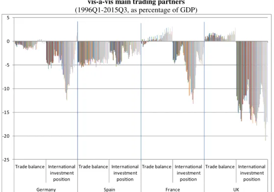
We assess the evolution of the bilateral trade balance as well as the bilateral IIP for the period 1996Q1-2015Q3. We consider the main trading partners of the Portuguese economy (Figure 8).7
In the case of Germany, there were trade balance deficits during many quarters of the period of analysis and a negative IIP. However, recently there has been equilibrium in both the trade balance and the IIP. Concerning Spain, the sum of the negative trade balance was stronger than the negative IIP.
On the other hand, the trade balance vis-à-vis France and the UK has been positive. Therefore, the negative IIP meant that France and the UK have been financial intermediaries of investments from the ROW. This conclusion is in line with Hobza &
6 We do not include the Portuguese stock market index (PSI-20) to avoid potential endogeneity with the
dependent variable.
7 In the analysis of the international investment position, we consider “Direct investment” and “Portfolio
20
Zeugner (2014). In the recent period, the main financier of the Portuguese economy has been the UK, while Germany has reduced exposure to Portuguese debt and equity.
[Figure 8]
Regarding the IIP vis-à-vis offshore financial centres, there was an increasing positive position of Portugal vis-à-vis these centres from 1996 until the financial crisis in 2009 and a reduction from thereon.
7. Conclusions
The aim of this study was to assess the sustainability of the Portuguese external accounts as well as the role of the public sector over the period 1999-2014.
The trade balance saw an increase during the EFAP from a strong deficit to a slight surplus. Concerning the bilateral trade balances, there was a persistent trade deficit vis-à-vis Spain. In the recent period, there was a trade surplus vis-à-vis France, the UK and the Portuguese-speaking African countries.
The deceleration of potential output had an impact on the decrease of the non-cyclical imports. Concerning the imported content based on the error correction model, investment was the component most dependent on imports, followed by exports, private consumption and public consumption. Additionally, we disaggregate investment between construction and non-construction as well as between public and private investment. There was evidence of higher import content in non-construction investment. This was an additional challenge to the Portuguese economy because its increase did not create a strong positive multiplier effect on the domestic economy. Furthermore, a positive evolution of the ratio between the GDP deflator and the import deflator was correlated with higher imports.
With respect to the exports variation, there was a positive impact from the economic growth of the euro area, in which the increase of the Portuguese exports was stronger than the economic growth rate of the euro area. In addition, the lagged variation of the share of the Portuguese nominal exports in the total exports of the euro area had a positive impact on the Portuguese export growth. Increases in the Portuguese market share make it easier for the country to benefit from the growth of the euro area in the future. This share recovered after 2011. Furthermore, the decomposition of the lagged ULC of the private sector presents marginal statistical significance: the growth of employees’
21
compensation and real productivity. The appreciation of the euro was statistically significant. Finally, the lagged variation of the terms of trade was beneficial to the exports in volume.
We analysed the determinants of the liabilities related to the IIP: direct investment and portfolio investment disaggregated by debt and equity. In this way, we know how net borrowing was financed. During the EFAP, the other investment instrument increased due to the external official debt from international institutions (EU/IMF).
The weight of the ratio between portfolio investment’s liabilities and direct investment’s liabilities was positively explained by the financial integration in the euro area and negatively explained by the EFAP.
The portfolio investment debt’s liabilities were positively correlated with financial integration in the euro area. However, there was a negative relationship with the degree of openness, trade balance and Portuguese 10-year sovereign yield due to the price effect and the EFAP dummy variable.
Concerning the liabilities of the direct investment equity, they were positively explained by the financial integration in the euro area as well as by the US stock market. On the other hand, there was a negative relationship with the measure of financial stress in Europe, the 3-month Euribor rate, appreciation of the euro (EUR/USD) and Portuguese 10-year sovereign yield.
Regarding the portfolio investment equity’s liabilities, there was a positive impact from the US stock market and the other investment position. However, there has been a negative effect related to the period after the financial crisis in 2009 as well as from the Portuguese 10-year sovereign yield.
There was a negative correlation between internal and external balances, i.e. when there was an internal balance (imbalance) there was an external imbalance (balance). This negative correlation was verified between private employment and trade balance. Furthermore, the output gap and unemployment rate presented a negative correlation, which is in line with the Okun's law.
In addition, there was no evidence of twin deficit during the period of analysis. The correlation between budget deficit and trade balance was weak. This conclusion is in line with the low import content of public consumption and the low level of public investment. The impact of the public sector on external accounts has the following channels: direct
22
effect through imported public consumption and investment, indirect effect through incentives and the environment for private entrepreneurship with the aim of increasing export growth, interest payments to non-resident holders related with public debt and transfers with the EU.
Finally, it is important to stress that there was a trade surplus vis-à-vis France and the UK, but there was a negative IIP, which meant that these countries were financial intermediaries between the ROW and Portugal.
8. References
Abbott, A. J., and H. R. Seddighi. “Aggregate imports and expenditure components in the UK: an empirical analysis.” Applied Economics, 1996: 1119-1125.
Afonso, António, and Jorge Silva. “Current account balance cyclicality.” Applied
Economics Letters, 2017: 911-917.
Afonso, António, Christophe Rault, and Christophe Estay. “Budgetary and External Imbalances Relationship: a Panel Data Diagnostic.” Journal of Quantitative Economics, January-July 2013: 84-110.
Bayoumi, Tamim, Richard Harmsen, and Jarkko Turunen. “Euro Area Export Performance and Competitiveness.” IMF working paper, June 2011.
Berger, Helge, and Volker Nitsch. “Wearing corset, losing shape: The euro’s effect on trade imbalances.” Journal of Policy Modeling, 2014: 136-155.
Blanchard, Olivier. “Current Account Deficits in Rich Countries.” International
Monetary Fund, 30 October 2006.
—. “Adjustment within the euro. The difficult case of Portugal.” Portuguese Economic
Journal, 2007: 6:1-21.
Chen, Ruo, Gian Maria Milesi-Ferretti, and Thierry Tressel. “Eurozone external imbalances.” Economic Policy, January 2013: 101-142.
Funke, Katja, and Christiane Nickel. “Does fiscal policy matter for the trade account? A panel cointegration study.” European Central Bank, May 2006.
Hobza, Alexandr, and Stefan Zeugner. “The ‘imbalanced balance’ and its unravelling: current accounts and bilateral financial flows in the euro area.” European Commission:
Economic Papers 520, July 2014.
Lane, Philip R., and Gian Maria Milesi-Ferretti. “External adjustment and the global crisis.” Journal of International Economics, 4 January 2012: 252-265.
23
Lebrun, Igor, and Esther Pérez. “Real Unit Labor Costs Differentials in EMU: How Big, How Benign and How Reversible?” International Monetary Fund Working Paper, May 2011.
Salto, Matteo, and Alessandro Turrini. “Comparing alternative methodologies for real exchange rate assessment.” DG ECFIN, European Commission, September 2010.
Figure 1 – Portugal: current account and non-cyclical current account (as percentage of GDP)
Source: BdP – Banco de Portugal, INE – Statistics Portugal and own calculations.
Figure 2 – Trade balance: Portugal vis-à-vis main trading partners (as percentage of GDP, moving average 4 quarters)
Source: BdP – Banco de Portugal, INE – Statistics Portugal and own calculations. In the case of OPEC, trade balance includes only goods. In this graph, Angola is included in the Portuguese-Speaking African Countries instead of the OPEC.
-15 -12 -9 -6 -3 0 3 M a r-1 9 9 6 D e c -1 9 9 6 S e p -1 9 9 7 Ju n -1 9 9 8 M a r-1 9 9 9 D e c -1 9 9 9 S e p -2 0 0 0 Ju n -2 0 0 1 M a r-2 0 0 2 D e c -2 0 0 2 S e p -2 0 0 3 Ju n -2 0 0 4 M a r-2 0 0 5 D e c -2 0 0 5 S e p -2 0 0 6 Ju n -2 0 0 7 M a r-2 0 0 8 D e c -2 0 0 8 S e p -2 0 0 9 Ju n -2 0 1 0 M a r-2 0 1 1 D e c -2 0 1 1 S e p -2 0 1 2 Ju n -2 0 1 3 M a r-2 0 1 4 D e c -2 0 1 4 S e p -2 0 1 5
Current Account (% GDP) Non-cyclical current account (% GDP)
-12 -10 -8 -6 -4 -2 0 2 D e c -1 9 9 9 Ju n -2 0 0 0 D e c -2 0 0 0 Ju n -2 0 0 1 D e c -2 0 0 1 Ju n -2 0 0 2 D e c -2 0 0 2 Ju n -2 0 0 3 D e c -2 0 0 3 Ju n -2 0 0 4 D e c -2 0 0 4 Ju n -2 0 0 5 D e c -2 0 0 5 Ju n -2 0 0 6 D e c -2 0 0 6 Ju n -2 0 0 7 D e c -2 0 0 7 Ju n -2 0 0 8 D e c -2 0 0 8 Ju n -2 0 0 9 D e c -2 0 0 9 Ju n -2 0 1 0 D e c -2 0 1 0 Ju n -2 0 1 1 D e c -2 0 1 1 Ju n -2 0 1 2 D e c -2 0 1 2 Ju n -2 0 1 3 D e c -2 0 1 3 Ju n -2 0 1 4 D e c -2 0 1 4 Ju n -2 0 1 5
Total Germany Spain France Rest of the EMU UK Portuguese-speaking African Countries Rest of the world OPEC
Total Spain
Rest of the world Rest of the EMU Germany France Portuguese Speaking African Countries OPEC UK
24
Figure 3 – Portugal: private employment and trade balance (Thousands of people and percentage of GDP)
Source: INE – Statistics Portugal and own calculations.
Figure 4 – Portugal: nominal unit labour costs of the private sector (index 1999Q4=100, moving average 4 quarters)
.
Source: INE – Statistics Portugal and own calculations. Notes: Ratio of compensation per employee in the private sector to real GVA per person employed in the private sector.
-14 -12 -10 -8 -6 -4 -2 0 2 3200 3400 3600 3800 4000 4200 4400 4600 M a r-1 9 9 8 M a r-1 9 9 9 M a r-2 0 0 0 M a r-2 0 0 1 M a r-2 0 0 2 M a r-2 0 0 3 M a r-2 0 0 4 M a r-2 0 0 5 M a r-2 0 0 6 M a r-2 0 0 7 M a r-2 0 0 8 M a r-2 0 0 9 M a r-2 0 1 0 M a r-2 0 1 1 M a r-2 0 1 2 M a r-2 0 1 3 M a r-2 0 1 4 M a r-2 0 1 5
Private employment (left) Trade balance-to-GDP (right)
80 90 100 110 120 130 140 150 D e c -1 9 9 9 S e p -2 0 0 0 Ju n -2 0 0 1 M a r-2 0 0 2 D e c -2 0 0 2 S e p -2 0 0 3 Ju n -2 0 0 4 M a r-2 0 0 5 D e c -2 0 0 5 S e p -2 0 0 6 Ju n -2 0 0 7 M a r-2 0 0 8 D e c -2 0 0 8 S e p -2 0 0 9 Ju n -2 0 1 0 M a r-2 0 1 1 D e c -2 0 1 1 S e p -2 0 1 2 Ju n -2 0 1 3 M a r-2 0 1 4 D e c -2 0 1 4 S e p -2 0 1 5
Real GVA per employment: private sector ULC nominal: private sector
25
Figure 5 – Portugal: international investment position - main items by financial instrument (end-of-period, outstanding amounts, percentage of GDP)
Source: BdP – Banco de Portugal, INE – Statistics Portugal and own calculations.
Figure 6 – Portugal: decomposition of direct and portfolio investment into equity and debt (liabilities as percentage of GDP)
Source: BdP – Banco de Portugal, INE – Statistics Portugal and own calculations. -140 -120 -100 -80 -60 -40 -20 0 20 40 M a r-1 9 9 6 D e c -1 9 9 6 S e p -1 9 9 7 Ju n -1 9 9 8 M a r-1 9 9 9 D e c -1 9 9 9 S e p -2 0 0 0 Ju n -2 0 0 1 M a r-2 0 0 2 D e c -2 0 0 2 S e p -2 0 0 3 Ju n -2 0 0 4 M a r-2 0 0 5 D e c -2 0 0 5 S e p -2 0 0 6 Ju n -2 0 0 7 M a r-2 0 0 8 D e c -2 0 0 8 S e p -2 0 0 9 Ju n -2 0 1 0 M a r-2 0 1 1 D e c -2 0 1 1 S e p -2 0 1 2 Ju n -2 0 1 3 M a r-2 0 1 4 D e c -2 0 1 4 S e p -2 0 1 5 International investment position Direct investment Portfolio investment Financial derivatives and employee stock options Other investment Reserve assets 0 20 40 60 80 100 120 M a r-1 9 9 6 De c -1 9 9 6 S e p -1 9 9 7 Ju n -1 9 9 8 M a r-1 9 9 9 De c -1 9 9 9 S e p -2 0 0 0 Ju n -2 0 0 1 M a r-2 0 0 2 De c -2 0 0 2 S e p -2 0 0 3 Ju n -2 0 0 4 M a r-2 0 0 5 De c -2 0 0 5 S e p -2 0 0 6 Ju n -2 0 0 7 M a r-2 0 0 8 De c -2 0 0 8 S e p -2 0 0 9 Ju n -2 0 1 0 M a r-2 0 1 1 De c -2 0 1 1 S e p -2 0 1 2 Ju n -2 0 1 3 M a r-2 0 1 4 De c -2 0 1 4 S e p -2 0 1 5
Direct investment - equity Direct investment - debt Portfolio investment - equity Portfolio investment - debt
26
Figure 7 – External debt: disaggregation by instrument (percentage of GDP)
Source: BdP – Banco de Portugal, INE – Statistics Portugal and own calculations.
Figure 8 – Bilateral trade balance and bilateral international investment position – Portugal vis-à-vis main trading partners
(1996Q1-2015Q3, as percentage of GDP)
Source: BdP – Banco de Portugal, INE – Statistics Portugal and own calculations. Notes: The trade balance is a flow at nominal prices, while the IPP is a stock at market value.
0 50 100 150 200 250 M a r-1 9 9 6 D e c -1 9 9 6 S e p -1 9 9 7 Ju n -1 9 9 8 M a r-1 9 9 9 D e c -1 9 9 9 S e p -2 0 0 0 Ju n -2 0 0 1 M a r-2 0 0 2 D e c -2 0 0 2 S e p -2 0 0 3 Ju n -2 0 0 4 M a r-2 0 0 5 D e c -2 0 0 5 S e p -2 0 0 6 Ju n -2 0 0 7 M a r-2 0 0 8 D e c -2 0 0 8 S e p -2 0 0 9 Ju n -2 0 1 0 M a r-2 0 1 1 D e c -2 0 1 1 S e p -2 0 1 2 Ju n -2 0 1 3 M a r-2 0 1 4 D e c -2 0 1 4 S e p -2 0 1 5
Total External Debt Direct investment Portfolio investment Other investment
-25 -20 -15 -10 -5 0 5
Trade balance International investment
position
Trade balance International investment
position
Trade balance International investment position
Trade balance International investment
position
27
Table 1 – The q-o-q quarterly change of imports in volume – short run (base year: 2011, EUR millions)
Notes: t-statistics in brackets. *, **, *** denote significance at 10, 5 and 1% levels estimation. Heteroskedasticity and Autocorrelation Consistent Covariance (HAC) or Newey-West. Estimator: Error Correction Model – two steps.
Table 2 – Estimations of the y-o-y quarterly change of exports in volume (percentage points)
Notes: t-statistics in brackets. *, **, *** denote significance at 10, 5 and 1% levels estimation. Heteroskedasticity and Autocorrelation Consistent Covariance (HAC) or Newey-West estimator. Equations were estimated by OLS.
Variable (1) (2) (3) (4) (5) constant 24.44 19.94 -17.42 45.49** -9.61 (1.1) (1) (-0.7) (2.4) (-0.6) Δ private consumption 0.44*** 0.36*** 0.39*** (4.6) (4) (7.3) Δ public consumption -0.44* -0.21 -0.01 (-1.7) (-0.6) (-0.1)
Δ public and private consumption 0.28***
(4.2) Δ investment 0.8*** 0.83*** (14.2) (13.2) Δ public investment 0.9*** (13.5) Δ private investment 0.83*** (13.7) Δ investment: construction 0.31*** (4.9)
Δ investment: non construction 1.06***
(18.5)
Δ exports 0.55*** 0.57*** 0.57*** 0.6***
(8.9) (9.3) (9.3) (12.7)
Δ global demand 0.59***
(15.8)
Δ (GDP deflator to imports deflator) 1294.70 484.49 659.77 1248.30 2456.34***
(1.4) (0,5) (0.6) (1.5) (3.6) convergence rate -0.3*** -0.25*** -0.06* -0.33*** -0.49*** (-3.8) (-4.4) (-1.7) (-5.1) (-4.4) R-square 0.90 0.89 0.82 0.92 0.94 Durbin-Watson 2.27 2.29 2.37 2.15 2.01 Observations 82 82 82 66 82 Period 1995:2-2015:3 1995:2-2015:3 1995:2-2015:3 1999:2-2015:3 1995:2-2015:3 Variable (1) (2) (3) (4) (5) constant 1.41** 1.66** 1.39** 1.44** 0.74 (2.4) (2.6) (2) (2.5) (1.5) yoy terms of trade (t-4) 0.31* 0.3* 0.36* 0.35** 0.46***
(1.9) (1.8) (1.9) (2.4) (3.1) yoy real GDP euro area 2.26*** 2.33*** 2.38*** 2.29*** 2.26***
(12) (9.9) (10.6) (9.6) (10.7) yoy nominal ULC private sector (t-1) -0.39***
(-2.7)
yoy ULC compensation per employee private sector (t-1) -0.49** -0.47** -0.37* (-2.5) (-2.4) (-1.9) yoy ULC real productivity private sector (t-1) 0.32 0.35*
(1.6) (1.9) yoy ULC nominal productivity private sector (t-1) 0.12
(0.7)
Dummy EFAP 2.67** 2.55** 3.18*** 2.58** 3.79*** (2.6) (2.4) (3.4) (2.5) (4.2) yoy Portuguese exports in the euro area exports (t-1) 0.43*** 0.42*** 0.4*** 0.51*** 0.54***
(4.1) (4.1) (3.2) (4.9) (4.6) yoy EUR/USD -0.06** -0.06*** (-2.5) (-2.8) R-square 0.83 0.84 0.83 0.84 0.84 Durbin-Watson 1.69 1.74 1.68 1.89 1.81 Observations 62 62 62 62 62 Period 2000:2-2015:3 2000:2-2015:3 2000:2-2015:3 2000:2-2015:3 2000:2-2015:3
28
Table 3 – Estimations of the of the q-o-q quarterly change of the ratio between Portfolio investment and Direct investment
(liabilities, percentage points)
Notes: t-statistics in brackets. *, **, *** denote significance at 10, 5 and 1% levels estimation. Heteroskedasticity and Autocorrelation Consistent Covariance (HAC) or Newey-West estimator. Equations were estimated by OLS.
Table 4 – Estimations of the q-o-q quarterly change of the portfolio investment: debt (liabilities, percentage points of GDP)
Notes: t-statistics in brackets. *, **, *** denote significance at 10, 5 and 1% levels estimation. Heteroskedasticity and Autocorrelation Consistent Covariance (HAC) or Newey-West estimator. Equations were estimated by OLS.
Variable (1) (2) (3)
constant 1.50 2.49** 2.24**
(1.6) (2.6) (2.1)
Δ cross holdings of government bonds 3.99** 3.63** 4.26***
(2.4) (2.7) (3) Δ degree of openness -1.37** -0.91 (-2.3) (-1.4) Δ trade balance-to-GDP -2.3* -1.84 (-1.7) (-1.6) Dummy EFAP -3.94* -3.3* -4.33** (-2) (-1.7) (-2.2)
Δ IIP balance of the Other investment-to-GDP 1.33*** 1.41***
(6.7) (7.4) R-square 0.24 0.42 0.39 Durbin-Watson 2.19 2.04 1.89 Observations 59 59 59 Period 2000:2-2014:4 2000:2-2014:4 2000:2-2014:4 Variable (1) (2) (3) constant 1.52*** 1.88*** 1.77*** (3.8) (4.9) (4.5)
Δ cross holdings of government bonds 1.38* 1.25*** 0.99**
(1.9) (2.7) (2.2) Δ degree of openness -0.75*** -0.58** -0.55** (-3.3) (-2.7) (-2.5) Δ trade balance-to-GDP -0.98* -0.82* -0.66 (-1.7) (-1.7) (-1.3) Dummy EFAP -1.82* -1.59* -1.67* (-2) (-1.9) (-1.9)
Δ IIP balance of the Other investment-to-GDP 0.48*** 0.45***
(6.4) (5.7)
Δ Portuguese sovereign yield 10 years (t-1) -0.75**
(-2)
R-square 0.36 0.55 0.57
Durbin-Watson 1.91 1.78 1.84
Observations 59 59 59
29
Table 5 – Estimations of the q-o-q quarterly change of the direct investment: equity (liabilities, percentage points of GDP)
Notes: t-statistics in brackets. *, **, *** denote significance at 10, 5 and 1% levels estimation. Heteroskedasticity and Autocorrelation Consistent Covariance (HAC) or Newey-West estimator. Equations were estimated by OLS.
Table 6 – Estimations of the q-o-q quarterly change of the portfolio investment: equity (liabilities, percentage points of GDP)
Notes: t-statistics in brackets. *, **, *** denote significance at 10, 5 and 1% levels estimation. Heteroskedasticity and Autocorrelation Consistent Covariance (HAC) or Newey-West estimator. Equations were estimated by OLS.
Variable (1) (2) (3)
constant 0.28** 0.26** 0.27**
(2.1) (2.2) (2.2)
Δ Euribor 3 month -0.76* -0.93** -0.86**
(-1.8) (-2.4) (-2.2)
Δ cross holdings of corporate bonds 0.79** 0.71** 0.67**
(2.3) (2.1) (2)
Δ CISS -5.17*** -5.38*** -4.98***
(-5.2) (-4.7) (-4.5)
q-o-q variation S&P 500 index (t-2) 0.04*** 0.04***
(2.9) (2.9)
q-o-q variation EUR/USD (t-2) -0.05** -0.06**
(-2) (-2)
Δ 10-year Portuguese sovereign yield (t-1) -0.14
(-0.8) R-square 0.26 0.35 0.36 Durbin-Watson 1.83 1.96 1.94 Observations 59 59 59 Period 2000:2-2014:4 2000:2-2014:4 2000:2-2014:4 Variable (1) (2) (3) constant 0.09 0.38** 0.27 (0.5) (2) (1.4)
Δ IIP balance of the Other investment-to-GDP 0.13** 0.13** 0.1**
(2.4) (2.6) (2.1)
q-o-q variation S&P 500 index (t-2) 0.11*** 0.12*** 0.11***
(4.9) (5.2) (5.1)
Dummy financial crisis -0.88*** -0.8**
(-2.7) (-2.6)
Δ Portuguese sovereign yield 10 years (t-4) -0.61***
(-3.3)
R-square 0.32 0.37 0.42
Durbin-Watson 1.80 1.95 2.01
Observations 78 78 78