Article
Printed in Brazil - ©2018 Sociedade Brasileira de Química
*e-mail: [email protected]
Binary
Solvent
Dispersive
Liquid-Liquid
Microextraction
for
the
Determination
of
Pesticides
in
Natural
Water
Samples
PriscilaL.S.Estevão,aPatricioPeralta-Zamora*,aandNoemiNagataa
aDepartamento de Química, Universidade Federal do Paraná,
P.O. Box 19081, 81531-990 Curitiba-PR, Brazil
A binary solvent dispersive liquid-liquid microextraction (BS-DLLME) technique was developed for simultaneous determination of diuron, teflubenzuron, atrazine, and two of its metabolites (desisopropylatrazine and desethylatrazine) in natural waters. The extraction was investigated using a three components mixture design to determine the best ratio between the extractors (dichloromethane and chloroform) and the disperser solvent (acetonitrile). According to the analysis of variance, empirical response surfaces were obtained for each analyte, correlating the absolute recovery and the mixture composition. The analysis of the overlapping surfaces allowed the detection of the best condition for the analytes extraction: 481 µL of chloroform, 56.6 µL of dichloromethane, 906 µL of acetonitrile, 5.00 mL of the aqueous sample, and 10% (m/v) of sodium chloride. The proposed method was validated and successfully applied in the analysis of surface waters, presenting suitable linearity (r > 0.9990), low limits of detection (0.015 to 0.36 µg L-1) and quantification (0.049 to 1.2 µg L-1), and relative recoveries between 84.8 and 106.1%.
Keywords: binary solvent dispersive liquid-liquid microextraction, pesticides, natural waters, mixture design
Introduction
In the last years, the focus of the environmental monitoring has been directed to a large group of organic pollutants,1 many of which can produce harmful effects
at low concentration such as endocrine disruption.2 In
the context of endocrine disrupting compounds (EDCs), it is relevant to remark the use of pesticides, herbicides, insecticides, and fungicides, in the pest control in agriculture. When applied to crops, these compounds can be transported over long distances via different mechanisms, especially precipitation, leaching, volatilization, and surface water runoff. Therefore, pesticides drift into aquatic environments contaminating ground and surface waters.3
Between 2008 and 2013, Brazil stood out as the world’s largest consumer of pesticides,4,5 due to the intensive
agricultural production, given prominence to grains crops like corn, soybeans, and wheat. Therefore, atrazine (ATZ), diuron (DIU), and carbendazim, which are allowed in these crops, are frequently among the top-ten most sold active ingredients in Brazil.6 As a consequence of the high
consumption and the inadequate use and residual disposal,
the contamination of surface and consumption waters has already been reported in several Brazilian states, especially in areas of high agricultural production.7-9
In general, these chemical species show high toxicity and persistence in the environment, which justifies the efforts dedicated to establish routines that allow their quantification in environmental matrices. Several techniques have been employed for pesticides determination in water samples,10 such as solid phase extraction (SPE),11,12
stir bar sorptive extraction (SBSE),13,14 and liquid-phase
microextraction (LPME)15 techniques, such as the
dispersive liquid-liquid microextraction (DLLME).16-19
Developed by Rezaee et al.20 in 2006, the DLLME is a
rapid extraction method that provides high recovery rates (especially for non-polar analytes), ease of operation, and also low cost, which is a feature inherent to all liquid-liquid extractions (LLE).
Several changes have been introduced to DLLME,21-27
some aiming to overcome the recovery problems in the simultaneous determination of analytes with broad polarity range. For instance, the use of two or three extractor solvents has been implemented by several authors.28-32
by employing the conventional LLE procedures because of the difficulty of finding an adequate solvent system. Wang et al.29 employed 100 µL of chloroform:undecanol
(1:1) for the determination of nicotine (log Kow 1.17) and cotinine (log Kow 0.07) in urine using DLLME with the solidification of a floating organic drop (SFO). If compared to the isolated use of the solvents, the recovery of cotinine, which is the most polar analyte in the system, was improved. Farajzadeh and Khoshmaram30 were the first to
use a ternary solvents mixture to evaluate the migration of phthalates (log Kow 1.6 to 6.6) from plastic food packaging. The extractor solvent mixture included chloroform (CLF, 404 µL), dichloromethane (DCM, 122 µL) and carbon tetrachloride (44 µL), and 2 mL of dimethylformamide as the disperser solvent. Under optimized conditions, the absolute recoveries (ARs) varied from 20-90%, for samples of mineral water, lemon juice, dough, vinegar, yogurt, and soda.
This study evaluates the potential of DLLME in the extraction of pesticides of different polarities, using a binary extractor solvent system (chloroform and dichloromethane), and acetonitrile (ACN) as a disperser solvent. The selected pesticides were: diuron (DIU, phenyl urea herbicide, log Kow 2.9), teflubenzuron (TFB, benzoylurea insecticide,
log Kow 4.3), atrazine (ATZ, triazine herbicide, log Kow 2.7)
and its two main metabolites, desisopropylatrazine (DIA, log Kow 1.1) and desethylatrazine (DEA, log Kow 1.5). The
effect of the solvent mixture composition was evaluated using a mixture design, which is a statistical tool that allows evaluating several variables simultaneously and also to investigate the interaction between them, ensuring the optimization with a smaller number of experiments.33 This
kind of experimental design allows the measurement of the effect of different mixture compositions in the response of interest. The proportions of the constituents in the mixture are mutually dependent and the sum of the components is limited to 100%. The mixture design is broadly applied in the pharmaceutical industry, in food analysis,34,35 and in the
optimization of experiments such as the solvent extraction of bioactive compounds from natural products36,37 and in
sample preparation.29,30,38
Experimental
Reagents
All standards were purchased from Sigma-Aldrich with purity higher than 96%. Stock solutions of each analyte were prepared in methanol (HPLC grade, 99.99%, J.T.Baker, Phillipsburg, USA) in a concentration of 100 mg L-1, and
were kept under refrigeration at –20 °C. From these stock
solutions, working solutions were freshly prepared by appropriate dilution of the initial mobile phase composition in ultrapure water (18.2 MΩ cm, Millipore Simplicity UV, Bedford, MA, USA). HPLC grade solvents used as extractor solvents were chloroform and dichloromethane (99.99%, Sigma-Aldrich, St. Louis, USA), and the one used as a disperser solvent was acetonitrile (99.99%, J.T.Baker, Phillipsburg, USA). Sodium chloride was puriss p.a. grade (≥ 99.8%, Sigma-Aldrich, St. Louis, USA).
Chromatographic analysis
The chromatographic analyses were carried out on a high-performance liquid chromatography (LC) Varian 920-LC (Mulgrave, Australia), equipped with an autosampler, quaternary gradient pump, diode array detector (DAD) and GALAXIE software v 1.9. The chromatography separation was carried out on a C18 analytical column (250 × 4.6 mm, 5 µm particle size, Microsorb-MV100-5) with a C18 guard column. The sample injection volume was set at 50 µL, the flow rate was 1.0 mL min-1, and the
column temperature was kept at 40 °C. The gradient elution mode was developed for the simultaneous determination of the analytes using acetonitrile:water (v/v). The initial mobile phase composition (40:60 acetonitrile:water) was kept constant for the first 8 min, then was linearly altered to 90% of acetonitrile at 15 min remaining at this composition until 20 min, and linearly returned to the initial conditions at 23 min. External analytical curves were elaborated using the mobile phase (40:60 acetonitrile:water) as solvent, in the concentration range of 2.5 to 2500 µg L-1. The DAD
monitoring wavelengths were 215 nm for DIA and DEA, 223 nm for ATZ, 254 nm for DIU, and 200 nm for TFB.
Extraction procedure
Two mixture designs were performed to evaluate the best solvents composition (CLF, DCM, ACN in percentage) for the extraction of the analytes. Due to the different densities of the solvents employed (CLF 1.48 g mL-1;
DCM 1.33 g mL-1; ACN 0.786 g mL-1), the proportions
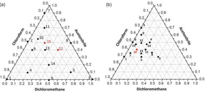
of the solvent mixtures were evaluated considering their mass and not their volume, setting 100% as 1.500 g of the extractor and disperser mixture solvents. The proportions used in each design are shown in Figure 1, and the response (absolute recovery of each analyte) was evaluated in Statistica software.39
with 30.0 µg L-1 of each analyte. These solutions were
prepared in 10% (m/v) sodium chloride to raise the ionic strength and facilitate the phase separation due to the salting-out effect.17,18 Quantities of salt higher than 10%
were not used, due to the precipitation of small crystals of NaCl in the interface between the organic and the aqueous phases after the centrifugation step.
The samples were vortexed (B. Braun Biotech International Vortex Certomat MV, Melsungen, Germany) for 30 s and then centrifuged for 6 min at 4400 rpm (Eppendorf centrifuge 5702, Hamburg, Germany). The vortex agitation was set at 30 s since the simple solvent addition with the micropipette did not present reproducible results in preliminary tests. Also, the speed and time of centrifugation were previously optimized in order to promote the complete phases separation. Afterwards, all sediment phase was collected with a glass syringe, transferred to a 2 mL vial, dried under a gentle flow of nitrogen, re-dissolved in 250 µL of mobile phase (ACN:H2O, 40:60), and analyzed by LC-DAD.
After the optimization by mixture design, the effect of the total solvent mass on the pesticides recovery was performed employing 0.800; 1.00; 1.25; 1.50; 1.75 and 2.00 g of the solvent mixture, keeping agitation, centrifugation, drying and re-dissolving conditions as previously described.
Real sample analysis
Spring water (latitude: 24°48’31.8”; longitude: 50°03’11.9”) and river sample (Iapó River, latitude 24°41’07.0”; longitude: 49°52’13.8”) were collected in Castro City (east of Paraná State, Brazil). All the samples were filtered through 0.45 µm glass fiber membrane
(Macherey-Nagel, Düren, Germany), added with 1 mL L-1
of methanol to avoid the microorganisms proliferation, and stored in brown glass bottles at 4 °C before analysis. After filtration, the soluble fractions were analyzed by the optimized method. The samples were fortified with six different levels of each analyte (0.50-100 µg L-1,
n = 3) by adding the appropriate volume of the stock solutions. The fortified samples were submitted to the binary solvent-dispersive liquid-liquid microextraction-liquid chromatography with diode array detection (BS-DLLME-LC-DAD) method in up to 48 h to perform the matrix-matched calibration. Matrix-matched calibration was performed in both real samples and in ultrapure water, at the same fortification levels.
Results and Discussion
Chromatographic analyses and standard calibration
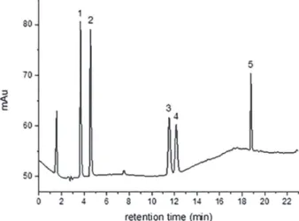
The analytes were separated by LC-DAD (Figure 2) on a C18 column under acetonitrile:water gradient elution with a suitable resolution. The quantification was performed via external standard calibration (n = 3) using independent curves prepared in the gradient initial composition (40:60, acetonitrile:water). The detectability of the chromatographic method was evaluated using the external analytical curves (Table 1). The linear range (LR) is comprised between the instrumental limit of quantification (LOQ) and the upper limit of the calibration curve. The limits of detection (LOD) and quantification (LOQ) were estimated by the ratio between the standard deviation of the intercept (s) and the slope of the analytical curves (S), being LOD equal to 3 times
and LOQ to 10 times the s/S ratio. Low instrumental limits of detection (LODi < 3.0 µg L-1) and quantification
(LOQi < 10.0 µg L-1) were achieved, similar to those
described in the literature,40-43 recalling that until then,
no preconcentration step was performed. Furthermore, suitable linearity (r > 0.9997) was obtained in the studied LR for all compounds. The analytical curves presented a random dispersion of the residuals and significant regression with the ratio of the regression sum of squares (SSR) by the sum of squared residuals (SSr) superior to the Fcritical, according to the analysis of variance (ANOVA)
with 95% of confidence level. The absolute recoveries, used as response in the DLLME method optimization, were estimated utilizing the external standardization curves.
Binary solvent dispersive liquid-liquid microextraction process
The conventional DLLME employs only one extractor solvent, what often hinders the simultaneous extraction of analytes with a wide range of polarity. Preliminary tests for the simultaneous pesticides extraction were performed
using n-octanol, toluene, cyclohexane as extractor solvents, and four other disperser solvents, acetone, acetonitrile, methanol, and ethanol. However, better recoveries for the most polar analytes, DIA and DEA, were achieved by adding a more polar solvent, dichloromethane (log Kow 1.5),
to the extractor:disperser mixture solvents, which consisted of chloroform:acetonitrile (CLF log Kow 2.0:ACN
log Kow –0.33). These tests were performed with 0.300 mL
of CLF, 0.200 mL of DCM and 1.000 mL of ACN, and absolute recoveries between 31 and 74% were obtained. Therefore, the extraction BS-DLLME routine was investigated applying a simplex design to determine the best ratio between the extractors (CLF and DCM) and the disperser (ACN) solvents.
The simplex design is a kind of mixture design in which the components of the mixture are mutually dependent and their sum is limited to 100%.44 It allows the evaluation
of the effect of different mixture compositions on the response. In the case of a three components mixture (CLF, DCM, ACN in percentage), different combinations are arranged in a triangle, whose vertices correspond to the pure components (100%), the edges represent the binary mixtures, and the points inside the triangle to the ternary mixtures. Empiric models can be built by the least squares method, making it possible to estimate the response for a given composition of the mixture, provided that it is comprised in the experimental design.
The volume of solvent was converted to mass of solvent using the values for density, and it was possible to estimate the mass as 0.444 g of CLF; 0.265 g of DCM and 0.786 g of ACN employed in the preliminary test. Therefore, the total mass of solvent used was 1.495 g, corresponding to a ratio in % (m/m) of 29.7% CLF, 17.7% DCM, and 52.6% ACN. Hence, there were two mixture designs for three variables, and the 1.500 g of mixture solvents (CLF, DCM, ACN in percentage) was fixed at 100%.
At this optimization step, the studied response was the absolute recovery (AR) of the analytes, estimated by the ratio between the observed (Co) and the expected
concentration (Ce):
Table1. Analytical parameters of external standard calibration and retention time of analytes
Analyte Retention time / min LR / (µg L-1) r Slope LOD
i / (µg L-1)
DIA (215 nm) 3.67 2.9-2500 0.9998 0.00720 0.87
DEA (215 nm) 4.58 7.9-2500 0.9999 0.00475 2.4
ATZ (223 nm) 11.59 4.9-2500 0.9996 0.00635 1.5
DIU (254 nm) 12.31 10.0-2500 0.9997 0.00277 3.0
TFB (200 nm) 18.84 7.6-2500 0.9993 0.00487 2.3
LR: linear range; r: correlation coefficient; LODi: instrumental limit of detection; DIA: desisopropylatrazine; DEA: desethylatrazine; ATZ: atrazine; DIU: diuron; TFB: teflubenzuron.
(reference 45) (1)
(2)
where FL is the concentration of the fortification level, Vs
is the volume of sample (5.00 mL), and Vr is the volume
of mobile phase redissolution (0.250 mL).
Design 1
The conditions employed in the first mixture modeling and the ARs obtained in each assay are shown in Figure 1a and described in Table 2. These compositions were selected to simultaneously evaluate the effect of the two extractors solvents without the disperser solvent (i.e., the points at the triangle vertices), the individual effect of the extractor solvent with the disperser solvent (i.e., points at the edges), and the effect of the combination of the two extractors solvents with the disperser solvent at different ratios (i.e., internal points in the diagram).
The assay 15, which has similar conditions to the preliminary test using CLF:DCM:ACN, was carried out in triplicate to estimate the variance, thus totaling 17 experiments. Phase separation was not obtained in the assay employing pure ACN.
In the absence of ACN (assay 2) it was not possible
to recover any of the analytes in concentrations above the LOQ of the chromatographic method. This result shows the importance of the disperser to the rapid establishment of an equilibrium between the solvent phases, allowing adequate recoveries in short extraction times.46 In assays
1 and 3, satisfactory recoveries were obtained (> 70%) for most analytes, in spite of the absence of the disperser. However, large quantities of CLF and DCM were employed: 1.01 and 1.13 mL, respectively. Therefore, among all experiments, assay 15 allowed good recoveries for the analytes with relatively lower consumption of chlorinated solvents. Besides, a significant improvement in the analytes extraction was observed in this assay compared to the preliminary CLF:DCM:ACN assays, where no NaCl was employed, thus evidencing the salting-out effect. Nonetheless, good recoveries were observed in assays 10 and 13, which conditions are similar to those used in assay 15, indicating that this region may present the best analyte extraction performance.
Furthermore, the difficulty of interpreting the individual results obtained in this design indicates the existence of an interaction between them. Thereby, the effect of the mixture components on the recoveries and the possibility of obtaining valid empirical models were assessed using an ANOVA with 95% of confidence level. However, valid models were not obtained due to the wide range of the mixture composition evaluated in this design. Therefore,
Table2. Conditions employed in design 1 and absolute recoveries of each pesticide
Assay % (m/m/m) Absolute recovery / %
CLFa DCMb ACNc DIAd DEAe ATZf DIUg TFBh
1 100 0.000 0.000 51.1 83.4 99.3 99.5 67.7
2 50.0 50.0 0.000 < 0.48i < 1.3i < 0.82i < 1.7i < 1.3i
3 0.000 100 0.000 48.8 78.9 96.0 96.7 82.5
4 70.0 20.0 10.0 52.3 80.1 96.9 96.3 59.6
5 20.0 70.0 10.0 28.3 43.8 52.3 53.1 33.8
6 0.000 50.0 50.0 < 0.48i < 1.3i < 0.82i < 1.7i < 1.3i
7 10.0 0.000 90.0 30.5 48.2 78.8 82.9 53.9
8 50.0 0.000 50.0 45.2 69.7 90.0 91.4 46.3
9 50.0 10.0 40.0 49.0 73.0 94.6 95.0 59.3
10 35.0 10.0 55.0 39.7 59.7 81.0 82.5 51.4
11 20.0 10.0 70.0 52.3 77.5 103.0 100.4 < 1.3i
12 20.0 40.0 40.0 39.3 ± 1.2j 104.5 ± 2.2j 83.4 ± 1.4j 91.9 ± 1.2j 45.0 ± 0.65j
13 35.0 25.0 40.0 50.8 74.6 96.0 94.0 52.7
14 40.0 40.0 20.0 51.6 78.2 94.9 94.6 62.2
15 30.0 20.0 50.0 48.8 ± 2.3k 72.7 ± 3.1k 91.7 ± 4.2k 95.1 ± 4.5k 64.3 ± 5.8k
another design was performed to obtain valid empirical models close to the optimum region, as shown in Figure 1b. The assay 10, which is displayed in red, was performed in triplicate.
Design 2
A simplex constrained mixture design was performed to evaluate in detail the best recovery sub-region, with lower and upper limits being delimited for the solvent mixture proportions. Thus, the chosen conditions were converted into pseudo-components, which simplifies the adjustment of the empirical models,44 so that the proportions
varied from 0.000 to 100%. The results for each condition (Figure 1b) are shown in Table 3.
Quadratic empirical models evaluated by ANOVA were well fitted for representing the absolute recovery rate of the analytes (DIA, DEA, ATZ, DIU, and TFB) as a function of the solvent proportions (extractor and disperser). In the case of TFB (less polar analyte), 12 assays from the design 1 were also considered to obtain the valid model. The parameters of the model are shown in Table 4.
The quadratic models obtained showed satisfactory percentage of explained variance, taking into account the percentage of maximum variance explainable by the model for all analytes. In addition, all regressions were significant at 95% of confidence level since the MSRegression/MSresidual (Fregression) ratio, where MS is the
mean square, was higher than Fcritical (3.11 to DIA, DEA,
ATZ, DIU models and 2.68 to TFB). Furthermore, no lack of fit was observed in any models, with MSlackoffit/MSpureerror(Flackoffit) lower than Fcritical (19.32 to
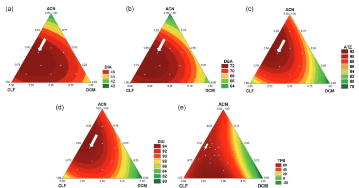
DIA, DEA, ATZ and DIU models and 4.604 to TFB). Besides, the residues produced by all empirical models were low and random, confirming the suitability of the models. Hence, response surfaces were built (Figure 3) to demonstrate the dependence of the analytes recoveries on the different proportions of solvents evaluated.
The best ratio of solvents for the simultaneous extraction of analytes can be determined by overlapping the response surfaces. This ratio is 47.5% CLF:5.00% DCM:47.5% ACN (point 15 of design 2), indicated by the white arrows in Figure 3. Under these conditions the absolute recoveries (n = 3) were 49.4 ± 1.4% for DIA, 73.2 ± 1.2% for DEA, 95.1 ± 2.4% for ATZ, 94.7 ± 2.2% for DIU and 74.9 ± 1.5% for TFB.
Total solvent weight
The influence of the amount by weight of the solvents mixture in the analytes recovery was conducted employing 0.800; 1.00; 1.25; 1.50; 1.75 and 2.00 g of mixture solvents. These assays were performed at the proportion of best performance obtained by mixture modeling (47.5% CLF, 5.00% DCM and 47.5% ACN). The absolute recoveries are shown in Figure 4.
Table3. Absolute recoveries obtained for pesticides extraction in mixture design 2
Assay % (m/m/m) Absolute recovery / %
CLF DCM ACN DIA DEA ATZ DIU TFB
1 70.0 0.000 30.0 44.6 69.6 81.1 85.0 56.7
2 50.0 20.0 30.0 46.6 71.2 87.6 90.7 60.6
3 30.0 40.0 30.0 43.5 65.6 78.5 80.8 53.4
4 30.0 20.0 50.0 46.1 69.3 86.8 89.8 58.1
5 30.0 0.000 70.0 39.8 62.5 86.1 90.7 57.3
6 50.0 0.000 50.0 46.3 70.4 91.1 93.4 61.3
7 60.0 5.00 35.0 47.1 72.3 88.3 90.3 63.8
8 35.0 30.0 35.0 44.9 68.4 83.1 85.2 61.6
9 35.0 5.00 60.0 42.7 65.9 86.2 88.4 58.2
10 50.0 10.0 40.0 48.5 ± 0.68a 74.3 ± 1.1a 91.9 ± 1.8a 95.8 ± 1.8a 61.1 ± 1.6a
11 40.0 20.0 40.0 41.9 62.8 77.7 80.3 54.7
12 40.0 10.0 50.0 48.8 74.0 92.7 97.2 61.1
13 35.0 17.5 47.5 45.4 69.4 87.1 90.6 58.8
14 47.5 17.5 35.0 47.2 72.0 89.2 91.2 73.9
15 47.5 5.00 47.5 48.1 73.4 92.3 96.1 74.1
As seen in Figure 4, no significant differences were observed in the ARs of ATZ, DIU, and TFB when the total mass of solvent was varied, although smaller amounts of mixture solvent significantly reduced the recovery of DIA and DEA, which would increase their LODs and LOQs. Furthermore, larger quantities did not provide a significant increase in the absolute recovery rates. Hence, the total
weight of 1.500 g was maintained (i.e., using 481 µL of CLF, 56.6 µL of DCM and 906 µL of ACN). In this optimized condition, the volume of the organic extract obtained was 772 ± 19 µL (n = 6), which allowed the drying time under nitrogen flow to be below 15 min in a system developed in the laboratory capable of drying 12 samples simultaneously.
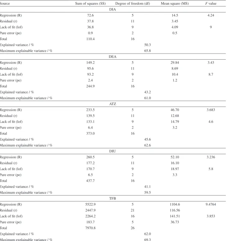
Table4. ANOVA parameters for the quadratic empirical models obtained for the analytes by mixture modeling
Source Sum of squares (SS) Degree of freedom (df) Mean square (MS) F value
DIA
Regression (R) 72.6 5 14.5 4.24
Residual (r) 37.8 11 3.45
Lack of fit (lof) 36.8 9 4.09 9
Pure error (pe) 0.9 2 0.5
Total 110.4 16
Explained variance / % 50.3
Maximum explainable variance / % 65.8
DEA
Regression (R) 149.2 5 29.84 3.43
Residual (r) 95.6 11 8.69
Lack of fit (lof) 93.2 9 10.4 8.7
Pure error (pe) 2.4 2 1.2
Total 244.9 16
Explained variance / % 43.2
Maximum explainable variance / % 61.0
ATZ
Regression (R) 233.5 5 46.70 3.683
Residual (r) 139.5 11 12.68
Lack of fit (lof) 133.1 9 14.79 4.6
Pure error (pe) 6.4 2 3.2
Total 373.0 16
Explained variance / % 45.6
Maximum explainable variance / % 62.6
DIU
Regression (R) 260.5 5 52.10 3.236
Residual (r) 177.2 11 16.10
Lack of fit (lof) 170.7 9 18.97 5.8
Pure error (pe) 6.5 2 3.3
Total 437.7 16
Explained variance / % 41.1
Maximum explainable variance / % 59.5
TFB
Regression (R) 5522.9 5 1104.6 9.4764
Residual (r) 2447.9 21 116.56
Lack of fit (lof) 2264.2 16 141.51 3.853
Pure error (pe) 183.7 5 36.73
Total 7970.8 26
Explained variance / % 62.0
Maximum explainable variance / % 69.3
Analytical performance of the method and real samples analysis
The optimal BS-DLLME conditions were applied to natural water samples collected in the state of Paraná at two different sites in the Tibagi River basin. The Tibagi River is 550 km long and limits one of the 16 hydrographic basins in the state of Paraná. Intensive agriculture represents the primary economic activity of this region, with emphasis on the crops of corn, soybeans, and wheat,47 in which the use
of ATZ, DIU, and TFB is allowed in Brazil. These crops are the main responsible for the pesticide consumption in Paraná and utilized more than 70% of the pesticides marketed in the state between 2013 and 2015.48 Therefore,
this region has a high potential for contamination of the water resources, making the monitoring of pesticides essential.
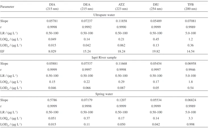
Table 5 summarizes the quantitative parameters of the BS-DLLME-LC-DAD obtained under optimized conditions in the ultrapure water and real samples (Iapó River and spring water). The enrichment factors (EFs) were estimated in ultrapure water by the ratio between the slopes of the calibration curves before (external standard calibration, Table 1) and after the BS-DLLME (matrix-matched calibration, Table 5).
The matrix-matched calibration curves were performed at six concentration levels (n = 3) and presented adequate linearity (r > 0.99) for all analytes in the respective LR. Furthermore, there were no notable differences between the curves obtained in real samples and in ultrapure water, confirming that the proposed method is not susceptible to the matrix effect in real samples.
Despite the lower EFs obtained in the BS-DLLME (8.029-19.82), this method showed LODm and LOQm values
similar to those described in the literature,12,19,49,50 as shown
in Table 6. In spite of providing high preconcentration factors, these methods have a high cost associated with the use of commercial cartridges or ionic liquids. Moreover, the method achieved LOQs similar to those obtained by GC-MS, known to be a more sensitive technique if compared to the DAD detection. In addition, the LOQ obtained for ATZ and DIU are lower than the limits established by the Brazilian legislation (2.0 and 90.0 µg L-1, respectively).51,52 Thus, the
proposed method is suitable and cheap for the determination of analytes in aqueous matrices, achieving merit parameters that are consistent with the literature.
Figure3. Level curves of the quadratic models to analytes absolute recovery as a function of solvent proportions (CLF:DCM:ACN). (a) DIA; (b) DEA; (c) ATZ; (d) DIU; (e) TFB.
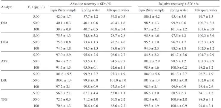
The trueness was evaluated using the absolute and relative recovery (RR) estimated by the ratio between the concentration obtained by matrix-matched calibration
(Cmm) and the concentration of the fortification level (FL),
according to equation 3, at three spiking levels performed in triplicate. These results and the respective standard
Table5. Analytical features of the matrix-matched calibration in ultrapure water and real samples
Parameter DIA
(215 nm)
DEA (215 nm)
ATZ (223 nm)
DIU (254 nm)
TFB (200 nm)
Ultrapure water
Slope 0.05781 0.07237 0.11858 0.05489 0.07081
r 0.9998 0.9992 0.9990 0.9999 0.9989
LR / (µg L-1) 0.50-100 0.50-100 0.50-100 0.50-100 5.0-100
LOQm / (µg L
-1) 0.049 0.14 0.21 0.45 1.2
LODm / (µg L-1) 0.015 0.042 0.062 0.13 0.36
EF 8.029 15.24 18.24 19.82 14.54
Iapó River sample
Slope 0.05881 0.07537 0.11668 0.05454 0.06958
r 0.9999 0.9997 0.9998 0.9997 0.9946
LR / (µg L-1) 0.50-100 0.50-100 0.50-100 0.50-100 5.0-100
LOQm / (µg L-1) 0.15 0.22 0.29 0.17 1.8
LODm / (µg L
-1) 0.046 0.066 0.087 0.05 0.54
Spring water
Slope 0.5786 0.07179 0.1207 0.05534 0.06824
r 0.9999 0.9998 0.9999 0.9999 0.9989
LR / (µg L-1) 0.50-100 0.50-100 0.50-100 0.50-100 5.0-100
LOQm / (µg L
-1) 0.051 0.37 0.17 0.14 3.3
LODm / (µg L-1) 0.015 0.11 0.050 0.042 0.998
DIA: desisopropylatrazine; DEA: desethylatrazine; ATZ: atrazine; DIU: diuron; TFB: teflubenzuron; r: correlation coefficient; LR: linear range; LOQm: limit of quantification of the method; LODm: limit of detection of the method; EF: enrichment factor.
Table6. Comparison of the proposed method with other methods
Analyte Method Sample volume / mL LODm / (µg L-1) LOQm / (µg L-1) EF Reference
DIA DEA ATZ
SPE-GC-MS 100
0.04 0.05 0.02
0.2 0.2 0.2
100 100 100
50
TFB MR-IL-DLLME-LC-UV 10 0.07 1 302 19
DIU SUPRAS-LC-DAD 10 0.13 0.43 48.5 49
DIA DEA ATZ
SPE-LC-DAD 10
0.12 0.09 0.09
0.04 0.03 0.03
25 12
DIA DEA ATZ DIU TFB
BS-DLLME-LC-DAD 5
0.015 0.042 0.062 0.13 0.36
0.049 0.14 0.21 0.45 1.2
8.029 15.24 18.24 19.82 14.54
proposed method
deviation (SD) are shown in Table 7.
(3)
The method presented satisfactory RR for all analytes in all samples, with values within the acceptable range of 70-120%. Higher SDs were also obtained in the lower concentrations, which was already expected due to the matrices complexity. However, the SDs for the determination of all analytes were lower than 6.3%. Furthermore, the similarity of the RR among the samples indicated a low matrix effect, which also indicates the stability of the method to small pH variations since the pH of the Iapó River sample (6.70) is distinct from the spring water sample (6.43).
No significant matrix effect was observed on the absolute recovery rates of the analytes. The matrix effect was verified by a one-way ANOVA using the absolute recovery means (50.0 µg L-1 of fortification level, n = 3)
of three different groups of samples: Iapó River, spring water, and ultrapure water. According to this test, there are no statistically significant differences in the ARs among the different samples at 95% of confidence level since the F values (MSbetweengroups/MSwithingroups) obtained for all
analytes were lower than the Fcritical value, which is 5.14 for
the df (degree of freedom) 2 and 6.
Although the sampling points are located in a region
of great agricultural production, in the analysis of samples without fortification (n = 3) none of the analytes were found in concentrations above the LODm. In addition,
no compounds eluted at the same retention time of the analytes in the blank samples, evidencing the selectivity of the method, as shown on the chromatograms in Figure 5.
Despite the presence of compounds eluting near the TFB, the peak is well resolved, evidencing the appropriate
Table7. Accuracy results for real samples analysis by BS-DLLME-LC-DAD method
Analyte FL / (µg L
-1) Absolute recovery ± SD
a / % Relative recovery ± SDb / %
Iapó River sample Spring water Ultrapure water Iapó River sample Spring water Ultrapure water
DIA
5.00 42.0 ± 1.7 37.7 ± 1.2 39.8 ± 0.5 106.1 ± 4.2 95.4 ± 3.0 99.7 ± 1.3
50.0 40.1 ± 0.3 40.1 ± 0.6 40.4 ± 1.6 98.5 ± 1.3 99.9 ± 0.6 100.7 ± 3.3
100 39.7 ± 0.9 40.7 ± 0.5 40.8 ± 0.4 97.3 ± 2.2 101.4 ± 1.2 101.6 ± 0.9
DEA
5.00 75.5 ± 1.3 74.8 ± 3.2 78.7 ± 2.8 95.8 ± 1.6 97.5 ± 4.2 100.3 ± 3.6
50.0 75.8 ± 0.8 73.4 ± 1.3 78.2 ± 4.6 95.5 ± 1.0 96.9 ± 1.7 102.3 ± 4.9
100 74.5 ± 1.8 74.5 ± 1.3 78.0 ± 0.9 94.0 ± 2.3 98.5 ± 1.8 102.3 ± 1.2
ATZ
5.00 97.0 ± 2.9 95.6 ± 2.5 96.6 ± 2.7 84.8 ± 3.2 101.7 ± 2.6 104.7 ± 2.9
50.0 94.9 ± 2.7 93.5 ± 1.1 94.5 ± 2.7 101.2 ± 2.9 98.5 ± 1.2 101.3 ± 2.9
100 91.7 ± 1.5 95.0 ± 0.1 92.6 ± 1.1 98.8 ± 1.6 100.0 ± 0.2 98.2 ± 1.2
DIU
5.00 101.6 ± 5.5 99.9 ± 2.7 97.3 ± 1.9 104.0 ± 5.6 101.3 ± 2.7 98.7 ± 1.9
50.0 100.0 ± 1.4 99.8 ± 0.8 101.0 ± 3.0 101.7 ± 1.4 100.1 ± 0.8 102.0 ± 3.0
100 97.2 ± 2.1 99.8 ± 0.9 97.5 ± 2.6 98.6 ± 2.1 99.9 ± 0.9 98.4 ± 2.6
TFB
5.00 56.3 ± 2.1 67.1 ± 4.4 55.0 ± 1.1 86.6 ± 3.0 88.5 ± 6.3 84.1 ± 1.5
50.0 72.5 ± 0.3 71.2 ± 2.0 70.8 ± 2.2 102.3 ± 0.4 100.9 ± 2.8 98.3 ± 3.1
100 70.6 ± 1.3 70.6 ± 0.6 68.6 ± 2.2 99.3 ± 1.9 100.4 ± 0.9 94.8 ± 3.1
aStandard deviation (n = 3) of the absolute recovery; bstandard deviation (n = 3) of the relative recovery. F
L: fortification level; DIA: desisopropylatrazine; DEA: desethylatrazine; ATZ: atrazine; DIU: diuron; TFB: teflubenzuron.
selectivity of the chromatographic method. The selectivity was also observed at 200 nm, which is the wavelength susceptible to the absorption of many organic interferents present in the sample. The DAD spectra and the retention time of the pure standards prepared in acetonitrile:water (40:60 v/v) were compared to those of the fortified real samples after the BS-DLLME. No difference between these parameters was observed, confirming the selectivity of the method.
The robustness of the proposed method was investigated using the Youden’s test,53 employing the Iapó River sample
fortified at 50.0 µg L-1. Seven parameters were evaluated
and the values for the effects of each factor in the absolute recovery are shown in Table 8.
The effects of the factors can be compared with the SD, obtained using the intermediate precision, associated with the tstudent value for the respective replicates number.
If the effects are lower than the SD × tstudent, they are not
significant.53 None of the effects obtained by the Youden’s
test (Table 8) was significant, indicating that the method is robust. Drying the extracts at 30 °C significantly reduced the time required in this step, and this condition was adopted in the optimized procedure, whereas the other conditions were maintained at the nominal levels of the Youden’s test.
Based on the outcomes of the validation tests, the developed BS-DLLME-LC-DAD method is suitable for the determination of all analytes in natural waters samples.
Conclusions
The three component mixture design allowed the development of a fast, cheap and sensitive BS-DLLME method to the determination of pesticides, including two metabolites of atrazine, with log Kow ranging between 1.1
and 4.3. The use of acetonitrile as a disperser solvent and two extractor solvents (chloroform and dichloromethane) improved the recovery of the more polar analytes, allowing suitable recoveries for the simultaneous determination of compounds with a wide range of polarity. The LOQs values of the method for ATZ (0.21 µg L-1) and DIU (0.45 µg L-1)
are, respectively, about 9.5 and 200 times lower than the limits established by the Brazilian legislation, indicating the capability of the method in detecting the pollutants in low concentrations. The method was validated and successfully applied to natural waters sampled in the state of Paraná, Brazil, without significant matrix effect.
Acknowledgments
The authors would like to express their gratitude to the CNPq (National Council for Scientific and Technological Development) and CAPES (Coordination for the Improvement of Higher Education Personnel) for their financial support and scholarship.
References
1. Jiang, J. Q.; Zhou, Z.; Sharma, V. K.; Microchem. J.2013, 110, 292.
2. Giulivo, M.; de Alda, M. L.; Capri, E.; Barceló, D.; Environ.
Res.2016, 151, 251.
3. Pal, A.; He, Y.; Jekel, M.; Reinhard, M.; Gin, K. Y. H.; Environ.
Int.2014, 71, 46.
4. Agência Nacional de Vigilância Sanitária (ANVISA);
Programa de Análise de Resíduos de Agrotóxicos em Alimentos (PARA) - Relatório de Atividades de 2011 e 2012; ANVISA: Brasília, 2013. Available at http://portal.anvisa.gov.br/ documents/111215/446359/Programa+de+An%C3%A1lise+d e+Res%C3%ADduos+de+Agrot%C3%B3xicos+-+Relat%C3
Table8. Absolute recovery effects for the parameters evaluated by the Youden’s test
Parameter Effect
DIA DEA ATZ DIU TFB
Flow (A: 1.0 mL min-1; a: 0.9 mL min-1) –3.57 –4.72 –5.97 –11.12 –6.78
Column temperature (B: 40 °C; b: 42.5 °C) –1.92 –2.98 –3.15 –0.56 –6.31
Drying temperature (C: room; c: 30 °C) 3.05 5.89 8.14 3.10 –1.89
Stirring time (D: 30 s; d: 25 s) –0.51 0.13 –2.50 –0.68 –0.42
Centrifugation time (E: 6 min; e: 5 min) –3.04 –4.64 –4.74 –4.85 3.58
Centrifugation speed (F: 4400 rpm; f: 4200 rpm) 0.08 0.14 2.15 1.19 4.83
%NaCl (G: 10% m/v; g: 9.5% m/v) 2.48 4.94 –9.49 –4.95 10.37
SD × tstudent (df = 2; 95% of confidence level) 4.29 8.66 15.3 16.5 10.5
%B3rio+2011+e+2012+%281%C2%BA+etapa%29/d5e91ef0-4235-4872-b180-99610507d8d5, accessed in April 2018. 5. Associação Brasileira de Saúde Coletiva (ABRASCO); Dossiê
ABRASCO - Um Alerta sobre os Impactos dos Agrotóxicos na Saúde; ABRASCO: Rio de Janeiro, 2012.
6. Instituto Brasileiro do Meio Ambiente e dos Recursos Naturais Renováveis (IBAMA); Boletim de Comercialização de Agrotóxicos e Afins - Histórico de Vendas - 2000 a 2012; IBAMA: Brasília, 2013.
7. Rocha, A. A.; Monteiro, S. H.; Andrade, G. C. R. M.; Vilca, F. Z.; Tornisielo, V. L.; J. Braz. Chem. Soc.2015, 26, 2269. 8. Moreira, J. C.; Peres, F.; Simões, A. C.; Pignati, W. A.; Dores,
E. C.; Vieira, S. N.; Strüssmann, C.; Mott, T.; Ciênc. Saúde Coletiva2012, 17, 1557.
9. Machado, K. C.; Grassi, M. T.; Vidal, C.; Pescara, I. C.; Jardim, W. F.; Fernandes, A. N.; Sodré, F. F.; Almeida, F. V.; Santana, J. S.; Canela, M. C.; Nunes, C. R. O.; Bichinho, K. M.; Severo, F. J. R.; Sci. Total Environ.2016, 572, 138.
10. Tankiewicz, M.; Fenik, J.; Biziuk, M.; TrAC, Trends Anal. Chem.
2010, 29, 1050.
11. Boulanouar, S.; Mezzache, S.; Combès, A.; Pichon, V.; Talanta
2018, 176, 465.
12. Cao, W.; Yang, B.; Qi, F.; Qian, L.; Li, J.; Lu, L.; Xu, Q.;
J. Chromatogr. A2017, 1491, 16.
13. Margoum, C.; Guillemain, C.; Yang, X.; Coquery, M.; Talanta
2013, 116, 1.
14. Assoumani, A.; Margoum, C.; Chataing, S.; Guillemain, C.; Coquery, M.; J. Chromatogr. A2014, 1333, 1.
15. Pinto, M. I.; Sontag, G.; Bernardino, R. J.; Noronha, J. P.;
Microchem. J.2010, 96, 225.
16. Martins, M. L.; Primel, E. G.; Caldas, S. S.; Prestes, O. D.; Adaime, M. B.; Zanella, R.; Sci. Chromatogr.2012, 4, 35. 17. Caldas, S. S.; Gonçalves, F. F.; Primel, E. G.; Prestes, O. D.;
Martins, M. L.; Zanella, R.; Quim. Nova2011, 34, 1604. 18. Nagaraju, D.; Huang, S. D.; J. Chromatogr. A2007, 1161, 89. 19. Zhang, J.; Li, M.; Yang, M.; Peng, B.; Li, Y.; Zhou, W.; Gao,
H.; Lu, R.; J. Chromatogr. A2012, 1254, 23.
20. Rezaee, M.; Assadi, Y.; Hosseini, M.-R. M.; Aghaee, E.; Ahmadi, F.; Berijani, S.; J. Chromatogr. A2006, 1116, 1. 21. Leong, M.-I.; Fuh, M.-R.; Huang, S.-D.; J. Chromatogr. A2014,
1335, 2.
22. Ahmad, W.; Al-Sibaai, A. A.; Bashammakh, A. S.; Alwael, H.; El-Shahawi, M. S.; TrAC, Trends Anal. Chem.2015, 72, 181. 23. Primel, E. G.; Caldas, S. S.; Marube, L. C.; Escarrone, A. L.
V.; Trends Environ. Anal. Chem.2017, 14, 1.
24. Trujillo-Rodríguez, M. J.; Rocío-Bautista, P.; Pino, V.; Afonso, A. M.; TrAC, Trends Anal. Chem.2013, 51, 87.
25. Gure, A.; Lara, F. J.; García-Campaña, A. M.; Megersa, N.; del Olmo-Iruela, M.; Food Chem.2015, 170, 348.
26. Hrouzková, S.; Brišová, M.; Szarka, A.; J. Chromatogr. A2017,
1506, 18.
27. Mansour, F. R.; Danielson, N. D.; Talanta2017, 170, 22. 28. Kiarostami, V.; Rouini, M.-R.; Mohammadian, R.; Lavasani,
H.; Ghazaghi, M.; Daru, J. Pharm. Sci.2014, 22, 25. 29. Wang, X.; Wang, Y.; Zou, X.; Cao, Y.; Anal. Methods2014, 6,
2384.
30. Farajzadeh, M. A.; Khoshmaram, L.; J. Chromatogr. A2015,
1379, 24.
31. Maham, M.; Karami-Osboo, R.; Kiarostami, V.; Waqif-Husain, S.; Food Anal. Methods2013, 6, 761.
32. Pastor-Belda, M.; Garrido, I.; Campillo, N.; Viñas, P.; Hellín, P.; Flores, P.; Fenoll, J.; Food Chem.2017, 233, 69.
33. Seabra, I. J.; Braga, M. E. M.; de Sousa, H. C.; J. Supercrit.
Fluids2012, 64, 9.
34. García-García, E.; Totosaus, A.; Meat Sci.2008, 78, 406. 35. Bueno, L.; Quim. Nova2008, 31, 306.
36. Handa, C. L.; de Lima, F. S.; Guelfi, M. F. G.; Georgetti, S. R.; Ida, E. I.; Food Chem.2016, 197, 175.
37. Anarjan, N.; Jouyban, A.; Food Bioprod. Process.2017, 103, 104.
38. Dorival-García, N.; Junza, A.; Zafra-Gómez, A.; Barrón, D.; Navalón, A.; Food Control2016, 60, 382.
39. Statistica, version 7.0; StatSoft, Tulsa, USA, 2004.
40. Leandro, C.; Souza, V.; Dores, E. F. G. C.; Ribeiro, M. L.;
J. Braz. Chem. Soc.2008, 19, 1111.
41. Yoon, J.-Y.; Park, J.-H.; Han, Y.; Lee, K.-S.; J. Agric. Chem. Environ.2012, 1, 10.
42. do Amaral, B.; de Araujo, J. A.; Peralta-Zamora, P. G.; Nagata, N.; Microchem. J.2014, 117, 262.
43. Santos, L. F. S.; Souza, N. R. S.; Ferreira, J. A.; Navickiene, S.; J. Food Compos. Anal.2012, 26, 183.
44. Neto, B. B.; Scarminio, I. S.; Bruns, R. E.; Como Fazer Experimentos - Pesquisa e Desenvolvimento na Ciência e na Indústria, 4a ed.; Bookman: Porto Alegre, 2010.
45. Instituto Nacional de Metrologia, Qualidade e Tecnologia (INMETRO); Orientação sobre Validação de Métodos
Analíticos, DOQ-CGCRE-008; INMETRO: Rio de Janeiro, 2010. Available at http://www.inmetro.gov.br/Sidoq/ Arquivos/CGCRE/DOQ/DOQ-CGCRE-8_03.pdf, accessed in April 2018.
46. Anthemidis, A. N.; Ioannou, K. I. G.; Talanta2009, 80, 413. 47. Secretaria de Estado do Meio Ambiente e Recursos Hídricos
(SEMA); Bacias Hidrográficas do Paraná; SEMA: Curitiba, 2010. Available at http://www.meioambiente.pr.gov.br/arquivos/ File/corh/Revista_Bacias_Hidrograficas_do_Parana.pdf, accessed in April 2018.
49. Scheel, G. L.; Tarley, C. R. T.; Microchem. J.2017, 133, 650. 50. Min, G.; Wang, S.; Zhu, H.; Fang, G.; Zhang, Y.; Sci. Total
Environ.2008, 396, 79.
51. Ministério da Saúde (MS); Portaria MS No. 2914 de 12 de dezembro de 2011, Dispõe sobre os Procedimentos de Controle e de Vigilância da Qualidade da Água para Consumo Humano e seu Padrão de Potabilidade; Brasília, DF, 2011. Available at http://bvsms.saude.gov.br/bvs/saudelegis/gm/2011/ prt2914_12_12_2011.html, accessed in April 2018.
52. Conselho Nacional do Meio Ambiente (CONAMA); Resolução No. 357, de 17 de março de 2005, Dispõe sobre a Classificação
dos Corpos de Água e Diretrizes Ambientais para o seu Enquadramento, bem como Estabelece as Condições e Padrões de Lançamento de Efluentes, e Dá Outras Providências; DOU: Brasília, Brasil, 2005. Available at http://www.mma.gov.br/port/ conama/legiabre.cfm?codlegi=459, accessed in April 2018. 53. Heyden, Y. V.; Nijhuis, A.; Smeyers-Verbeke, J.; Vandeginste,
B. G. M.; Massart, D. L.; J. Pharm. Biomed. Anal.2001, 24, 723.
Submitted: January 12, 2018 Published online: April 18, 2018