doi: 10.5540/tema.2018.019.01.0043
Different Numerical Inversion Algorithms of the Laplace Transform
for the Solution of the Advection-Diffusion Equation with
Non-local Closure in Air Pollution Modeling
†C. P. DA COSTA1*, K. RUI2and L. D. P ´EREZ-FERN ´ANDEZ1
Received on November 20, 2016 / Accepted on October 18, 2017
ABSTRACT. In this paper, a three-dimensional solution of the steady-state advection-diffusion equation is obtained applying the so-called generalized integral advection-diffusion multilayer technique, consid-ered non-local closure for turbulent flow. Two different parametrizations were considconsid-ered for the counter-gradient coefficient and three different methods of numerical inversion for inverse Laplace transform. The results were compared with the experimental data of Copenhagen experiment by an evaluation of statisti-cal indexes to analyze the solution of the equation through the methods of numeristatisti-cal inversion. Different parametrizations for the vertical turbulent eddy diffusivity and wind profile were utilized. The results show a good agreement with the experiment and the methods of numerical inversion for inverse Laplace transform show almost the same accuracy.
Keywords: Non-local closure, numerical inversion, pollutant dispersion.
1 INTRODUCTION
In the framework of pollutant dispersion modeling in the low atmosphere, Reynolds decomposi-tion applied to the equadecomposi-tion resulting from the law of conservadecomposi-tion of mass leads to an equadecomposi-tion exhibiting the so-called closure problem. In particular, it is necessary to provide constitutive relations linking pollutant concentration to the turbulent fluxes in the atmosphere. The tradi-tional approach is based on theK-theory, or gradient-transport theory, which states, in analogy to molecular diffusion, that the fluxes are proportional to the gradient of the mean pollutant concen-tration, providing the so-called local Fickian closure [32]. However, such an approach does not take into account the non-homogeneous character of turbulence in the planetary boundary layer (PBL), which occurs when convective movements are dominant. In fact,K-theory is known to
†Paper presented at the National Congress of Applied and Computational Mathematics 2016.
*Corresponding author: Camila Pinto da Costa – E-mail: [email protected].
1Departamento de Matem´atica e Estat´ıstica, DME – UFPel, Campus Universit´ario, 354, 96010-900 Pelotas, RS, Brasil. E-mail: [email protected]
fail in the presence of large-size eddies in the upper portion of the PBL, even though it has been commonly used in models that attempt to describe neutral-to-unstable atmospheric conditions [32]. Moreover, the derivation of theK-theory based on Prandtl’s mixing-length theory [26] is valid only for statically neutral situations [32]. Various approaches were developed to overcome such a situation. For instance, the nonlocal theories of spectral diffusivity [3] and transilient tur-bulence [31], which, although supported by some experimental evidence, produce results that differ from those of the statistical dispersion theory [32]. An alternative consist of considering the so-called nonlocal closure representing the counter-gradient fluxes to indicate the presence of scale eddies or nonlocal fluxes in the PBL [10, 11, 12]. In this context, one approach considers a Taylor expansion of the turbulent fluxes in the vertical direction [33, 35]. Here, we consider a linear closure for the counter-gradient term which is consistent with various experiment-based parametrizations of the counter-gradient fluxes [9, 10, 11, 12, 27].
From the methodological point of view, the boundary/initial-value problems for advection-diffusion equations with variable coefficients that model pollutant dispersion in the atmosphere are usually solved via integral transform-based methods [5, 6, 19, 20, 21, 34]. Among those meth-ods, the advection-diffusion multilayer method (ADMM) [19, 20] provides accurate analytical solutions. In fact, it was reported that the ADMM produces estimations of pollutant concentra-tions which are as accurate as other integral transform-based methods such as the generalized integral Laplace transform technique (GILTT) [21, 34] but with remarkably less computational cost [22]. This last feature is essential in real-life situations such as industrial/natural disasters which require swift (ideally real-time) and accurate estimations of the ground-level distribution and concentration of the pollutants escaped to the atmosphere.
The ADMM is based on the stepwise approximation of the continuous wind velocity profile and eddy diffusivity coefficients in the vertical direction. Such an approximation is the local aver-age of the variable coefficients over each sublayer. Then, the original problem with continuous coefficients is approximated by a problem with piecewise-constant coefficients and interlayer continuity conditions. The approximate problem is then analytically solved in the Laplace space, and the approximation of the solution of the original problem is obtained by applying the inverse Laplace transform to the analytical solution of the approximate problem in the Laplace space. For further details, see [20].
On the other hand, the GILTT relies on the Fourier method to produce an truncated eigenfunc-tion series expansion of the solueigenfunc-tion. As usual, the eigenfunceigenfunc-tions are obtained from the related Sturm-Liouville problem resulting via separation of variables. The coefficients of the series so-lution are obtained by solving an auxiliary problem for a matrix ordinary differential equation via the Laplace transform. This problem is obtained by using the orthogonality property of the eigenfunctions. Finally, the inverse Laplace transform is applied to this approximate solution in the Laplace space in order to obtain the approximation of the solution of the original problem. For further details, see [21].
closure. In particular, the GIADMT applies the GILTT in the crosswind lateral direction to the approximate problem resulting from the application of the ADMM. The resulting multilayer problem for the coefficients of the eigenfunction series expansion of the approximate solution is then solved in the Laplace space. Again, the approximation of the solution of the original problem follows by applying the inverse Laplace transform. For further details, see [6, 7].
As the solutions in the Laplace space provided by the three aforementioned methods are very complex, it is usually necessary to take a computational approach to the inversion of the Laplace transform. In models adopting the Fickian closure, we observed [28] that, when the solution is sought via the ADMM, the fixed-Talbot inversion algorithm [1] provides more accurate results than the Gaussian quadrature approach [30] and than a Fourier series-based method [8]. However, to the best of our knowledge, in models adopting non-Fickian closures, it has not been established which inversion algorithm of the Laplace transform is the most precise.
The objective of this work is twofold: to solve a steady-state three-dimensional advection-diffusion model with non-Fickian counter-gradient closure via the GIADMT, and to establish which inversion algorithm of the Laplace transform is the most accurate in this context. Here, we consider three inversion algorithms, namely, the Gaussian quadrature method [30], the fixed-Talbot method [1], and a Fourier series-based method [8]. Also, different parametrizations for the eddy diffusivities, the mean wind velocity profile, and the counter-gradient flux are considered in the numerical simulations, and the corresponding results are compared to the Copenhagen experiment dataset [15] via statistical analysis [17] in order to establish which parametrizations and inversion algorithm provide the most accurate results.
This work is organized as follows: section 2 is devoted to the derivation of the model; in section 3, the formalism of the GIADMT applied to the model is presented including the three inver-sion algorithms of the Laplace transform; the statistical validation of the model is described for various parametrizations of the coefficients and the the three inversion algorithms in section 4; the accuracy of the computational results is discussed in section 5; and concluding remarks are presented in section 6.
2 PROBLEM STATEMENT
Following [32, 36], the Eulerian approach (i.e. fixed reference system) to air pollution model-ing is based on the law of conservation of mass for one pollutant species with concentration
c(x,y,z,t):
∂c
∂t +u·∇c−D∆c=S, (2.1)
where(x,y,z)∈R+×[−Ly,Ly]×[0,h]are the spatial coordinates withLy,h>0,tis the temporal
coordinate,uis the wind velocity vector field,Dis the molecular diffusivity, andSis the pollutant source.
represent the mean and turbulent (i.e. fluctuating) parts, respectively. Such decompositions are justified by the existence of the so-called spectral gap, which is the lack of variation at temporal or spatial mesoscales and separates macroscalar mean motions from microscalar turbulent ones (for further details, see sections 2.2 and 2.3 of [32]). In addition, it is often assumed [32, 36] that an ergodic hypothesis [2] is satisfied by the turbulence (i.e. it is homogeneous and stationary, both statistically), soh(¯·)i=(¯·)andh(·)′i=0, whereh·idenotes the Reynolds average operator [32]. Also, turbulent motions smaller that the mesoscale, as the ones considered here, generally satisfy the conditions [4] for the so-called incompressibility approximation [16, 32], which produces the so-called continuity equation for turbulent fluctuations∇·u′=0, implying thatu′·∇c′=
∇·(c′u′). With such considerations, and by applying the average operator to equation (2.1), it follows that
∂c¯
∂t +u¯·∇c¯+∇· hc
′u′i −D∆c¯=hSi, (2.2)
wherehc′u′irepresents the turbulent atmospheric diffusion eddies. Also, as the dispersion effects of molecular diffusion are several orders of magnitude smaller than the ones corresponding to the turbulent diffusion eddies, it is possible to neglect termD∆c¯in equation (2.2) [32, 36].
On the other hand, observe that termhc′u′iintroduces three new unknowns, so equation (2.2) needs closure. The traditional approach is the so-calledK-theory, or gradient-transport theory, which relies on the so-called Fickian (or first-order local) closure, i.e.,hc′u′i=−K∇c¯, whereK is the second-rank tensor field of turbulent diffusion [32, 36]. However, when considering point sources in unstable atmospheric conditions, the Fickian closure presents major limitations, as its mixing-length derivation is valid only for statically neutral situations [32]. In order to overcome such a situation, we consider the nonlocal counter-gradient closurehc′u′i=−K(∇c¯−γ), where
γ is the so-called counter-gradient vector field [10, 11, 12]. With such considerations, and by assuming that the pollutant is nonreactive, sohSi=S, equation (2.2) becomes
∂c¯
∂t +u¯·∇c¯−∇·(K(∇c¯−γ)) =S. (2.3)
Further simplifications of equation (2.3) can be considered. For instance,Kis assumed to be a diagonal tensor with nonzero componentsKx,KyandKz[36]. Also, as the dominant convective
movements occur in the upward direction, the counter-gradient fieldγ is usually taken to be aligned to thez-axis, soγ= (0,0,γ)[11]. In addition, it is considered that thex-axis is aligned with the wind direction, so that ¯u= (u¯,0,0), and, in consequence, the turbulent diffusion along thex-axis is negligible in comparison to the corresponding advective transport:
¯
u∂c¯
∂x
≫
∂ ∂x
Kx
∂c¯
∂x
,
(2.4)
whereKx is the turbulent diffusivity along thex-axis. Also, in presence of a single pollutant
source in steady-state emission regime and atmospheric conditions, we have that∂c¯/∂t=0 and the source termS is treated as a boundary condition. With such considerations, equation (2.3) simplifies to
¯
u∂c¯
∂x−
∂ ∂y
Ky
∂c¯
∂y
−∂∂z
Kz
∂c¯
∂z−γ
whereKy andKz are the turbulent diffusivities along they- andz-axes, respectively. Equation
(2.5) is completed with the boundary condition accounting for the pollutant source
¯
uc¯|x=0=Qδ(z−Hs)δ(y), (2.6)
whereQis the emission rate of the pollutant source, which is located at point(0,0,Hs), andδ(·)
is Dirac’s delta function, and total reflexion conditions [36]:
Ky
∂c¯
∂y
y=±Ly
=0, (2.7)
and
Kz
∂ ¯
c
∂z−γ
z=0,h
=0. (2.8)
Finally, observe that the counter-gradient term γ is also unknown, so we propose the lin-ear closure γ =βc¯, which is consistent with various experiment-based parametrizations ofγ
[9, 10, 11, 12, 27]. Then, equations (2.5) and (2.8) become, respectively,
¯
u∂c¯
∂x−
∂ ∂y
Ky
∂c¯
∂y
−∂∂z
Kz
∂c¯
∂z
+ ∂
∂z(Kzβc¯) =0, (2.9)
and
Kz
∂ ¯
c
∂z−βc¯
z=0,h
=0. (2.10)
3 MODEL SOLUTION VIA GIADMT
The solution of problem (2.5)-(2.10) is sought via the GIADMT, which applies the GILTT in variableyto the multilayer problem resulting from the application of the ADMM. This problem for the coefficients of the eigenfunction series expansion of the approximate solution is then solved in the Laplace space. Finally, the approximation of the solution of the original problem follows by applying an inversion algorithm of the Laplace transform.
Following the formalism of the GILTT, the mean pollutant concentrationc(x,y,z)is sought as a Fourier series in terms of the eigenfunctionsψj(y), where jis the order of the corresponding
eigenvalueλj, that is,
c(x,y,z) =
∞
∑
j=0
Cj(x,z)ψj(y)
ψj , ψj 2 =
Z Ly
−Ly
ψ2j(y)dy. (3.1)
The eigenvaluesλjand the corresponding eigenfunctionsψj(y)in (3.1) are obtained by solving
the Sturm-Liouville problem
d2ψj
dy2 +λ
2
jψj(y) =0,
dψj
dy
y=
±Ly
=0, (3.2)
The coefficientsCj(x,z) of the Fourier series expansion of the mean pollutant concentration
c(x,y,z)are obtained by solving the problems resulting from the substitution of (3.1) into (2.9), (2.10) and (2.6), and considering the orthogonality of the eigenfunctions:
u∂Cj
∂x +Kyλ 2
jCj(x,z)−
∂ ∂z
Kz
∂Cj
∂z
+ ∂
∂z(KzβCj(x,z)) =0, (3.3)
Kz
∂
Cj
∂z −βCj(x,z)
z=0,h
=0, (3.4)
uCj(0,z) =
Q
p
Ly
δ(z−Hs). (3.5)
Now, we follow the formalism of the ADMM to find the solution of problem (3.3)-(3.5), that is, divide the heighthof the PBL intoNsublayers and then take the local average of coefficientsKy,
Kz,uandβin directionzover each sublayer. Explicitly, let{zn}n=0,N⊂[0,h]be a partition of the
PBL. In each sublayer(zn−1,zn),n=1,N, of thickness∆zn=zn−zn−1, consider the following
stepwise approximations ofu(z),Kτ(z),τ=y,z, andβ(z)given by
un=
1
∆zn
Z zn
zn−1
u(z)dz,Kτn=
1
∆zn
Z zn
zn−1
Kτ(z)dz,βn=
1
∆zn
Z zn
zn−1
β(z)dz.
Let Cjn(x,z) =Cj(x,z) for (x,z)∈R∗+×(zn−1,zn), n =1,N. Then, problem (3.3)-(3.5) is
approximated by the following ADMM problem:
un
∂Cjn
∂x +Kynλ 2
jCjn(x,z) =Kzn
∂2C
jn
∂z2 −Kznβn
∂Cjn
∂z ,z∈(zn−1,zn), (3.6) Cjn(x,zn) =Cj(n+1)(x,zn), (3.7)
Kzn
∂C
jn
∂z −βnCjn(x,z)
z=zn
=Kzn+1 ∂C
j(n+1)
∂z −βn+1Cj(n+1)(x,z)
z=zn
, (3.8)
Kz1 ∂C
j1
∂z −β1Cj1(x,z)
z=0
=KzN
∂C
jN
∂z −βNCjN(x,z)
z=h
=0, (3.9)
Cjn(0,z) =
Q unpLy
δ(z−Hs)δnn¯,z∈(zn−1,zn), (3.10)
in which conditions (3.7) and (3.8) follow from the continuity of the pollutant concentration and the turbulent flux in directionz, respectively, at the partition pointsz=zn,n=1,N−1. Also,δnn¯
in boundary condition (3.10) is Kronecker’s delta (δnn¯=1 ifn=n¯,δnn¯=0 ifn6=n¯), andn=n¯
By applying the Laplace transformL[·] in directionxto the ADMM problem (3.6)-(3.10), it follows, for eachs∈C, the ADMM problem in the Laplace space:
d2ζjn
dz2 −βn
dζjn
dz −
uns+Kynλ 2
j
Kzn
ζjn(s,z) =− Q Kzn
p
Ly
δ(z−Hs)δnn¯, (3.11)
ζjn(s,zn) =ζjn+1(s,zn), (3.12)
Kzn
dζ
jn
dz −βnζjn(s,z)
z=zn
=Kzn+1 dζ
jn+1
dz −βn+1ζjn+1(s,z)
z=zn
, (3.13)
Kz1 dζ
j1
dz −β1ζj1(s,z)
z=0
=KzN
dζ
jN
dz −βNζjN(s,z)
z=h
=0, (3.14)
whereζjn(s,z) =L[Cjn(x,z)]. Then, forz∈(zn−1,zn), n=1,N, the solution of the ADMM
problem in the Laplace space (3.11)-(3.14) is
ζjn(s,z) =Ajne
(Fn+Rjn)z+B jne
(Fn−Rjn)z+
+ Q
2RjnKzn
p
Ly
h
e(Fn−Rjn)(z−Hs)−e(Fn+Rjn)(z−Hs)iH(z−H
s), (3.15)
whereH(·)is Heaviside function,
Fn=−
βn
2 , Rjn=
s
β2
n
4 +
uns+Kynλ 2
j
Kzn
, (3.16)
and coefficientsAjn andBjn in (3.15) are obtained by solving the system of linear equations
resulting from the substitution of (3.15) into conditions (3.12)-(3.14).
Then, the solution of the ADMM problem (3.6)-(3.10) follows from the application of the inverse Laplace transformL−1[·]to (3.15), so the approximate solution to the original problem
(2.5)-(2.10) is, formally,
c(x,y,z) =
∞
∑
j=0
cos(λjy)
p
Ly
L−1[ζj](x,z). (3.17)
However, note that the complexity of solution (3.15) requires the numerical inversion of the Laplace transform, so the final solution is regarded as semi-analytic. In this work, three inver-sion algorithms are considered, namely, the Gaussian quadrature method [30], the fixed-Talbot method [1], and a Fourier series-based method [8], in order to establish inversion algorithm pro-vides the most accurate results. The applications of the three algorithms to (3.15) are described next:
• Gaussian quadrature method [30]:
cn(x,y,z) =
∞
∑
j=0
cos(λjy)
p
Ly
(Np
∑
k=1 pkwk
x ζjn
pk
x,z
)
, (3.18)
• Fixed-Talbot method [1]:
cn(x,y,z) =
∞
∑
j=0
cos(λjy)
p Ly r M∗ 1
2ζjn(r,z)e
rx+
+
M∗−1
∑
k=1
RehexS(θk)ζ
jn(S(θk),z)(1+iw(θk))
i #)
, (3.19)
where r is a parameter with value fixed as r=2M∗/101x, and S(θk) =rθ(cotθ+i),
ω(θk) =θk+ (θkcotθk−1)cotθk,θk=kπ/M∗,−π<θk<+π, andi2=−1.
• Fourier series-based method [8]:
cn(x,y,z) =
∞
∑
j=0
cos(λjy)
p
Ly
eαx
T
"N∗
∑
k=1 Re ζjnα+ikπ
T ,z
cos
kπx
T − −Im ζjn
α+ikπ
T ,z
sin
kπx
T
+1
2ζjn(α,z)
, (3.20)
whereα andT are free parameter taken here asα=0.0001 andT=55000.
4 MODEL VALIDATION
In order to validate the semi-analytical approach described above, parametrizations must be pro-vided for the eddy diffusivitiesKyandKz, the mean wind velocity profileu, and the
counter-gradient coefficientβ. The following parametrizations of are valid for the considered atmospheric convective conditions. ForKz:
• Pleim and Chang [25]:
Kz
w∗h=κ
z h
1−hz, (4.1)
whereκ=0.4 is von K´arm´an constant, andw∗is the convective velocity scale.
• Degrazia et al. [14]:
Kz
w∗h =0.22
z
h
1/3
1−hz1/3h1−e−4z/h−0.0003e8z/hi, (4.2)
• Degrazia et al. [13]:
Kz
w∗h=
0.09c1w/2ψ1/3(z/h)4/3
(fm∗)4w/3
Z ∞
0
sin
7.84c1/2w ψ1/3(fm∗)
2/3
w X n (z/h)2/3
(1+n′)5/3
dn′
n′ , (4.3)
whereψ=1.26 exp(−z/0.8h)is the non-dimensional molecular dissipation rate associ-ated to the plume production, cv,w=0.4, n′=nˆ(1.5z/u(fm∗)w) with frequency ˆn, X is
the non-dimensional time as it is the travel time ratex/u and the convective time scale
h/w∗, (fm∗)w =z/(λm)w is the spectral peak non-dimensional frequency, and (λm)w =
Also, forKy, we use the following parametrization:
• Degrazia et al. [14]:
Ky=
√
πσvz
16(fm)vqv
, (4.4)
with
σ2
v =
0.98cv
(fm)
2/3
v
ψ
ε
qv
2/3z
h
2/3
w2∗, (4.5)
ψε1/3=
1−z
L
2
−z L
−2/3 +0.75
1/2
, (4.6)
whereu∗is the friction velocity,Lis the Monin-Obukhov length,σv is the standard
de-viation of the longitudinal turbulent velocity,(fm)v=0.16 is the lateral wave peak,ψεis
the non-dimensional molecular dissipation rate,qv=4.16z/his the stability function, and
cv=0.4.
For the wind velocity profileu, we use the two parametrization by Panofsky and Dutton [24]:
• Power-law profile:
u=u1
z
z1
p
, (4.7)
whereuandu1are wind velocities at heightszandz1, respectively, whereaspis related to
the intensity of the turbulence [18].
• Logarithmic profile:
u=
(
(u∗/κ) [ln(z/z0)−Ψm(z/L)], z≤zb
(u∗/κ) [ln(zb/z0)−Ψm(zb/L)], z>zb
, (4.8)
wherez0is the roughness length of the terrain,zb=min[|L|,0.1h]and, with
A= [1−16(z/L)]1/4,Ψmis the stability function
Ψm=ln
1+A2
2
+ln
1+A
2 2
−2 arctanA+π
2. (4.9)
For the counter-gradient coefficientβ, we use the following two parametrization.
• Cuijpers and Holtslag [9]:
β=bw
2
∗
σ2
wh
, (4.10)
with constantband the vertical standard deviation of the turbulent velocityσw[29]:
σ2
w=1.8
z
h
2/3 1−z
h
2/3
• Roberti et al. [27]:
β=0.085qw
Ψh
h
z
2/3
, (4.12)
with non-dimensional dissipationΨ=0.913, andqwis the stability function
qw=z
h
0.594h1−e−4z/h−0.0003e8z/hi−1. (4.13)
Model validation is carried out by comparing the simulation results to the Copenhagen experi-ment observations [15]. This experiexperi-ment consisted of releasing sulfur hexafluoride (SF6) from a
source of heighth=115mand emission rateQ=100g/s. Nine experiments were carried out under moderately unstable atmospheric conditions, and data were collected at arches located at 2−6kmfrom the source. The roughness length isz0=0.6m. The comparison is performed via statistical analysis using the following indexes [17]:
• Normalized mean square error:
NMSE= (Co−Cp)2/CoCp (ideal:NMSE=0)
• Correlation coefficient:
Cor= [(Co−Co)(Cp−Cp)]/σoσp (ideal:Cor=1)
• Factor of two:
Fa2=Cp/Co∈[0.5,2] (ideal:Fa2=1)
• Fractional bias:
Fb= (Co−Cp)/(0.5(Co+Cp)) (ideal:Fb=0)
• Fractional standard deviation:
Fs= (σo−σp)/(0.5(σo+σp)) (ideal:Fs=0)
where subscripts o and p denote the experimentally observed and computationally predicted quantities, respectively,σ is the standard deviation, and the overbar represents the mean value.
5 RESULTS
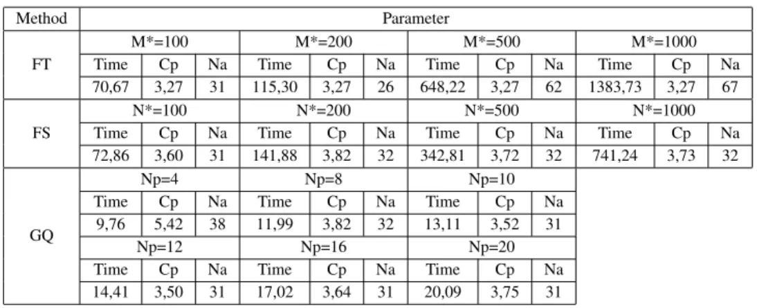
The numerical methods inversion of the Laplace transform, require parameter choices that have direct impact on the performance, e.g. the number of terms in the Fourier series (N∗), the number of terms in the Fixed-Talbot expansion (M∗), and the number of points used for the Gaussian quadrature (N p).
In order to determine the choice of such parameters was analysed of the computational cost that each method takes to determine the pollutant concentration given by the equation (3.17). For these tests, was utilized the power wind profile, diffusion coefficientKz of equation (4.3), term
3 of Copenhagen [15];y=0 andz=0. The value of the concentration observed in this arc is
Co=3.76.
Table 1 shows the time that each inversion method took to calculate the concentration, the value of the concentration obtained in each calculation and the number of eigenvalues required for GITT, and the criterion of the truncation of the sum of GITT is absolute error less than 10−2.
Table 1: Computational cost comparison of each inversion method.
Method Parameter
FT
M*=100 M*=200 M*=500 M*=1000
Time Cp Na Time Cp Na Time Cp Na Time Cp Na
70,67 3,27 31 115,30 3,27 26 648,22 3,27 62 1383,73 3,27 67
FS
N*=100 N*=200 N*=500 N*=1000
Time Cp Na Time Cp Na Time Cp Na Time Cp Na
72,86 3,60 31 141,88 3,82 32 342,81 3,72 32 741,24 3,73 32
GQ
Np=4 Np=8 Np=10
Time Cp Na Time Cp Na Time Cp Na
9,76 5,42 38 11,99 3,82 32 13,11 3,52 31
Np=12 Np=16 Np=20
Time Cp Na Time Cp Na Time Cp Na
14,41 3,50 31 17,02 3,64 31 20,09 3,75 31
Analyzing the table (1), it can be seen that the fixed-Talbot method has equal values of Cp inde-pendent of the number of expansion terms, in addition, the calculated value for Cp is very close to Co, but it is a method that takes more time to perform the calculations because it needs many eigenvalues. The higher the value ofM∗, the more eigenvalues are required. Thus, comparing accuracy/cost,M∗=100 is sufficient to calculate the concentration values.
The Fourier series-based method presents small changes in the values ofC pby increasing the number of terms in the series, moreover, the values calculated for Cp are also very close to Co. This method takes less time to perform the calculations than the fixed-Talbot method, because it does not need as many eigenvalues as the fixed-Talbot method. Thus,N∗=100 is sufficient to calculate the concentration values.
The Gaussian quadrature method is the fastest method to perform the calculations ofC p, but it is not due to the number of eigenvalues but because the number of points used in the present work is a maximum of twenty. The values calculated forC pvary according to the value ofNp
chosen, in addition, not always have values close toCo. It can be seen in Stroud-Secrest [30] that the magnitude of the real part of the root of the Gaussian quadrature scheme for the inverse Laplace transform increases withNp(the order of the approximation). Since the solution to the
concentration with the Laplace transform has exponential terms, one can readily observe that from the numerical simulation ”overflow” appears for the positive exponential argument and ”underflow” for the negative argument when Np assumes very high values. It is important to
Consequently, to avoid overflow and underflow, the values ofNpwere restricted to values around
twenty. Thus,N p=8 is sufficient to calculate the concentration values.
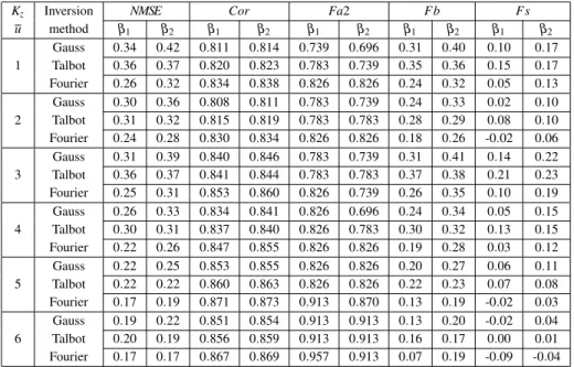
Once the parameters of each inversion method have been determined, the table (2) shows the statistical indexes of the approximate solutions (3.18), (3.19) and (3.20) considering all the parametrizations for the eddy diffusivitiesKy(equation (4.4)) andKz(equations (4.1), (4.2) and
(4.3)), the wind velocity profile (equations (4.7) and (4.8)), and the counter-gradient coefficient
β withβ1andβ2denoting the parametrizations in equations (4.10) and (4.12), respectively. The
corresponding computational experiments were performed by truncating the concentration series expansion in equations (3.18), (3.19) and (3.20) after 150 terms.
Table 2: Statistical indexes.
Kz Inversion NMSE Cor Fa2 Fb Fs
u method β1 β2 β1 β2 β1 β2 β1 β2 β1 β2
Gauss 0.34 0.42 0.811 0.814 0.739 0.696 0.31 0.40 0.10 0.17 1 Talbot 0.36 0.37 0.820 0.823 0.783 0.739 0.35 0.36 0.15 0.17 Fourier 0.26 0.32 0.834 0.838 0.826 0.826 0.24 0.32 0.05 0.13 Gauss 0.30 0.36 0.808 0.811 0.783 0.739 0.24 0.33 0.02 0.10 2 Talbot 0.31 0.32 0.815 0.819 0.783 0.783 0.28 0.29 0.08 0.10 Fourier 0.24 0.28 0.830 0.834 0.826 0.826 0.18 0.26 -0.02 0.06 Gauss 0.31 0.39 0.840 0.846 0.783 0.739 0.31 0.41 0.14 0.22 3 Talbot 0.36 0.37 0.841 0.844 0.783 0.783 0.37 0.38 0.21 0.23 Fourier 0.25 0.31 0.853 0.860 0.826 0.739 0.26 0.35 0.10 0.19 Gauss 0.26 0.33 0.834 0.841 0.826 0.696 0.24 0.34 0.05 0.15 4 Talbot 0.30 0.31 0.837 0.840 0.826 0.783 0.30 0.32 0.13 0.15 Fourier 0.22 0.26 0.847 0.855 0.826 0.826 0.19 0.28 0.03 0.12 Gauss 0.22 0.25 0.853 0.855 0.826 0.826 0.20 0.27 0.06 0.11 5 Talbot 0.22 0.22 0.860 0.863 0.826 0.826 0.22 0.23 0.07 0.08 Fourier 0.17 0.19 0.871 0.873 0.913 0.870 0.13 0.19 -0.02 0.03 Gauss 0.19 0.22 0.851 0.854 0.913 0.913 0.13 0.20 -0.02 0.04 6 Talbot 0.20 0.19 0.856 0.859 0.913 0.913 0.16 0.17 0.00 0.01 Fourier 0.17 0.17 0.867 0.869 0.957 0.913 0.07 0.19 -0.09 -0.04
logarithmicu,Kzof (4.1);2power-lawu,Kzof (4.1);3logarithmicu,Kzof (4.2);
4power-lawu,K
zof (4.2);5logarithmicu,Kzof (4.3);6power-lawu,Kzof (4.3).
It is observed in the table (2) that the three inversion algorithms studied provide results with similar precision for all parametrizations, since the values of all the statistical indices are close to the ideal values. These three methods are used to calculate the inverse of Laplace in this context of estimating the concentration of pollutants in the atmosphere. However, we can say that the Fourier series-based inversion algorithm produces better results even when comparing the computational effort with the other methods.
Figure 1 shows scatter plots of the observed pollutant concentrations(Co)from the Copenhagen
experiment versus the predicted concentrations(Cp) for the power-law wind velocity profile
computational experiment showed that the scatter plots in Figure 1 are representative of all the other parametrizations.
Cuijpers and Holtslag (1998) Roberti et al. (2004)
Figure 1: Scatter plots for power-law wind andKzof [13].
6 CONCLUSIONS
We presented the solution of the steady-state three-dimensional advection-diffusion equation with linear nonlocal closure via the GIADMT with two different parametrizations of the counter-gradient coefficient. Three numerical inversion algorithms of the Laplace transform were eval-uated: the Gaussian quadrature method, the fixed-Talbot method, and a Fourier series-based method. The use of non-local closure allowed to model satisfactorily the pollutant concentrations of the Copenhagen experiment independently of the choice of parametrizations and inversion al-gorithms. The statistical indexes showed that the accuracies of the three algorithms were similar, but the Fourier series-based method was the least expensive from the computational point of view.
ACKNOWLEDGMENTS
Financial support by FAPERGS is gratefully acknowledged.
a soluc¸˜ao da equac¸˜ao atrav´es dos m´etodos de invers˜ao num´erica. Ainda, foram utilizados diferentes parametrizac¸˜oes para o coeficiente de difus˜ao turbulento vertical e o perfil do vento. Os resultados apresentaram uma boa concordˆancia com o experimento e os m´etodos de invers˜ao num´erica para a transformada de Laplace apresentaram preaticamente a mesma precis˜ao, sendo que o m´etodo baseado na s´erie de Fourier foi o mais acurado dos trˆes algo-ritmos. Por outro lado, o m´etodo de fixed-Talbot foi o que mostrou o melhor desempenho do ponto de vista computacional.
Palavras-chave: Fechamento n˜ao-local, invers˜ao num´erica, dispers˜ao de poluentes.
REFERENCES
[1] J. Abate & P. Valk´o. Multi-precision Laplace transform inversion.Int. J. Numer. Methods Eng.,60 (2004), 979–993.
[2] M. Beran.Statistical Continuum Theories. John Wiley & Sons, New York, (1968).
[3] R. Berkowicz & L. P. Prahm. Generalization ofK-theory for turbulent diffusion. Part 1: Spectral turbulent diffusivity concept,J. Appl. Meteor.,18(3) (1976), 266–272.
[4] J. A. Businger. Equations & Concepts, in: F. T. M. Nieuwstadt, H. van Dop (Eds.) Atmospheric Turbulence and Air Pollution Modelling. Reidel, Dordrecht, (1982), 1–36.
[5] M. Cassol, S. Wortmann & U. Rizza. Analytical modeling of two-dimensional transient atmospheric pollutant dispersion by double GITT and Laplace Transform techniques,Environ. Model. Soft.,24 (2009), 144–151.
[6] C. P. Costa, M. T. Vilhena, D. M. Moreira & T. Tirabassi. Semi-analytical solution of the steady three-dimensional advection-diffusion equation in the planetary boundary layer.Atmos. Environ.,40(2006), 5659–5669.
[7] C. P. Costa, T. Tirabassi, M. T. Vilhena & D. M. Moreira. A general formulation for pollutant dispersion in the atmosphere.J. Eng. Math.,74(1) (2012), 159–173.
[8] K. S. Crump. Numerical Inversion of Laplace Transforms Using a Fourier series approximation.J. ACM,23(1) (1976), 89–96.
[9] J. W. M. Cuijpers & A. A. M. Holtslag. Impact of skewness and nonlocal effects on scalar and buoyancy fluxes in convective boundary layers,J. Atmos. Sci.,55(1998), 151–162.
[10] J. W. Deardorff. On the direction and divergence of the small-scale turbulent heat flux,J. Meteor.,18 (1961), 540–548.
[11] J. W. Deardorff. The counter-gradient heat flux in the lower atmosphere and in the laboratory,J. Atmosph. Sci.,23(1966), 503–506.
[13] G. A. Degrazia, D. M. Moreira & M. T. Vilhena. Derivation of an eddy diffusivity depending on source distance for vertically inhomogeneous turbulence in a convective boundary layer,J. Appl. Meteor., (2001), 1233–1240.
[14] G. A. Degrazia, U. Rizza, C. Mangia & T. Tirabassi. Validation of a new turbulent parameterization for dispersion models in convective conditions,Boundary-Layer Meteor.,85(2) (1997), 243–254.
[15] S. E. Gryning & E. Lyck.The Copenhagen Tracer Experiments: Reporting of Measurements. Riso National Laboratory, (2002).
[16] S. R. Hanna, G. A. Briggs & R. P. Hosker Jr.Handbook on Atmospheric Diffusion. U. S. Department of Energy, (1982).
[17] S. R. Hanna. Confidence limits for air quality models, as estimated by bootstrap and jackknife resampling methods.Atmos. Environ.,23(1989), 1385–1395.
[18] J. S. Irwin. A theoretical variation of the wind profile power-law exponent as a function of surface roughness and stability.Atmos. Environ.,13(1) (1979), 191–194.
[19] D. M. Moreira, U. Rizza, M. T. Vilhena & A. Goulart. Semi-analytical model for pollution dispersion in the planetary boundary layer.Atmos. Environ.,39(14) (2005), 2689–2697.
[20] D. M. Moreira, M. T. Vilhena, T. Tirabassi, C. P. Costa & B. Bodmann. Simulation of pollutant dis-persion in the atmosphere by the Laplace transform: The ADMM approach,Water, Air, Soil Pollut., 77(1) (2006), 411–439.
[21] D. M. Moreira, M. T. Vilhena, D. Buske & T. Tirabassi. The state-of-art of the GILTT method to simulate pollutant dispersion in the atmosphere,Atmos. Res.,92(1) (2009), 1–17.
[22] D. M. Moreira, M. T. Vilhena, T. Tirabassi, D. Buske & C. P. Costa. Comparison between analytical models to simulate pollutant dispersion in the atmosphere.Int. J. Environ. Waste Manag.,6, No. 3-4 (2010), 327–344.
[23] D. M. Moreira, A. C. Moraes, A. G. Goulart & T. T. A. Albuquerque. A contribution to solve the atmospheric diffusion equation with eddy diffusivity depending on source distance,Atmos. Environ., 83(2014), 254–259.
[24] A. H. Panofsky & A. J. Dutton.Atmospheric Turbulence, John Wiley & Sons, New York, 1984.
[25] J. Pleim & J. Chang. A non-local closure model for vertical mixing in the convective boundary layer, Atmos. Environ.,26A(6) (1992), 965–981.
[26] L. Prandtl. Bericht ¨uber Untersuchungen zur ausgebildeten Turbulenz,Z. angew. Math. Mech.,5(2) (1925), 136–139.
[27] D. R. Roberti, H. F. Campos Velho & G. A. Degrazia. Identifing counter-gradient term in atmospheric convective boundary layer.Inverse Probl. Sci. Eng.,12(3) (2004), 329–339.
[29] Z. Sorbjan.Structure of the Atmospheric Boundary Layer. Prentice Hall, (1989).
[30] A. H. Stroud & D. Secrest.Gaussian Quadrature Formulas. Prentice Hall, Inc., Englewood Cliffs, N. J., (1966).
[31] R. B. Stull. Transilient turbulence theory. Part 1: The concept of eddy mixing across finite distances, J. Atmos. Sci.,41(23) (1984), 3351–3367.
[32] R. B. Stull.An Introduction to Boundary Layer Meteorology. Kluwer Academic Publishers, Dordrecht, Holanda, (1988).
[33] H. van Dop & G. Verver. Countergradient transport revisited.J. Atmos. Sci.,58(15) (2001), 2240– 2247.
[34] S. Wortmann, M. T. Vilhena, D. M. Moreira & D. Buske. A new analytical approach to simulate the pollutant dispersion in the PBL.Atmos. Environ.,39(12) (2005), 2171–2178.
[35] J. Wyngaard & J. Weil. Transport asymmetry in skewed turbulence.Phys. Fluids A, 3(1) (1991), 155–162.