A Greedy Policy for Fleet-Level Radar Resource Management
Jinxin Zhao, Jinwoo Seok, Jhanani Selvakumar, Ricardo Bencatel,
Pierre Kabamba and Anouck Girard
Department of Aerospace Engineering
University of Michigan, Ann Arbor, Michigan 48109-2140
Email:{jinxinzh, sjinu, jhanani, bencatel, kabamba, anouck}@umich.edu
Abstract— A model for a phased-array radar in the context of a defensive Naval system has been developed using hierarchical finite state machines. This model is used to study resource management for a fleet of ships equipped with one radar unit each. This fleet is under attack from aerial enemy agents. A control algorithm formulated on this specific model is used to dynamically generate a greedy policy for radar operation. The defense system is evaluated in its capability to acquire and track those aerial threats, in two configurations -centralized and decentralized (independent). The performance is quantified on the basis of time taken to establish the threat trajectory, time to compute the policy and the number of threats the system fails to track. A comparison of performance in the two configurations is provided.
I. INTRODUCTION A. Motivation
The problem of radar resource management is significant to modern military systems. The era of fast and intelli-gent warfare necessitates use of complex radar systems with sophisticated detection and classification algorithms. A constraining factor is power utilization, particularly in offshore defense systems such as Naval vessels. In order to obtain a solution to the radar resource management problem that is feasible and matches performance standards, a radar model from the ONR has been adapted and an optimization procedure applied to it. The model is presented in this paper along with the control algorithm which generates a greedy policy for resource management.
B. Mission Overview
Consider a geographical area containing two forces: en-emy and friendly. The enen-emy force is composed of agents that pose a threat to the friendly force. The friendly force is composed of radar platforms, which are equipped to detect and track threats. The goals for the friendly force are to detect all the threats within the area, and to track all the detected threats. A practical radar model has been built and a control algorithm designed to fulfill these goals.
Jinxin Zhao, Jinwoo Seok, and Jhanani Selvakumar are graduate students, and Ricardo Bencatel is a post-doctoral research fellow, at the Department of Aerospace Engineering, University of Michigan, Ann Arbor, Michigan 48109-2140.
Pierre Kabamba and Anouck Girard are faculty at the Department of Aerospace Engineering, University of Michigan, Ann Arbor, Michigan 48109-2140.
C. Literature Review
A number of radar models exist at present. They corre-spond to different types of radars or are developed with spe-cific radar applications in consideration. One popular method of modeling radars is by Markovian processes. Visnevski et al [1] use a generalized semi-Markov process to model the emitter of a multi-function radar in application to electronic warfare. Watson and Blair [2] employ a Markov chain to mix state estimates from multiple models in their Interacting Multiple Model (IMM) algorithm. Ghosh et al [3] attempt to provide an integrated framework to optimize Quality of Service (QoS) and perform dynamic scheduling for radar systems with multiple resource constraints. A real-time dwell scheduling algorithm for a multifunction phased array radar using scheduling gain is presented by Ting et al [4]. It uses a combination of heuristics and scheduling gain. All of these papers consider a single radar unit capable of performing multiple functions simultaneously. In previous work [5], a method of building Dynamic Finite State Machines and solving the optimal policy using a Dynamic Programming method was presented.
In this paper we provide a radar model based on a hierarchical network of Finite State Machines. The principal idea of the model is that a phased array radar is an antenna that can transmit waveforms in any direction. The inputs to the model are radar pointing orientations and the amount of energy allocated to each orientation in an interval of time. The outputs are the parameters of the threats including position, velocity and heading. This radar model is subject to a scheduling control algorithm that, under power constraints, is capable of providing specific schedules for the radar, as required by the external environment.
D. Original Contributions
The original contributions of this paper are as follows: 1. A radar model that uses F inite State M achines: The use of abstract models of computation such as finite state machines makes the model amenable to studying radar configurations for fleets.
2. A control algorithm that provides a greedy policy f or operation: The control algorithm uses a step-by-step maximization algorithm applied to the finite state machine of the radar model. The output of the controller is a decision for radar orientation control and energy consumption at a particular time.
3. A comparative study of centralized and decentralized conf igurations: This paper compares these two modes of operation in the specific context of radar resource management. The comparison is facilitated by applying standard state machine composition to the radar model presented.
The modeling of fleets is relevant because employing fleets is ubiquitous in modern Naval operations. Unlike Markov process-based models, this model does not utilize probabilistic knowledge of the radars’ tracking capabilities. The control algorithm ensures that power utilization does not exceed the maximum power under any attack scenario. Also, re-evaluating the entire situation at each time step means that the radar is better equipped to handle the unpredictable nature of the threat dynamics. The comparative study provided here verifies that a centralized configuration gives the best possible performance and quantifies the difference in measure of performance between the centralized and decentralized cases. It also provides an insight into the tradeoff between the two.
E. Organization
The material in this paper is organized as follows: Section II provides background on finite state machines and the greedy algorithm. Section III presents the radar model and the control algorithm. Section IV describes in detail the problem and the specific assumptions that have been made. This is followed by the technical approach to the problem and a characterization of the decentralized and centralized modes of operation in Section V. Section VI contains simulation results that validate our method, and concluding remarks are found in Section VII.
II. THEORETICAL BACKGROUND A. Finite State Machines
To describe the battle situation, we use an FSM that con-structs the output signal one symbol at a time by observing the input signal one symbol at a time [6], [7], [8]. An FSM is a five-tuple:
F SM = (States, Inputs, Outputs, update, x0), (1)
where States, Inputs, and Outputs are sets, update is a function, and x0∈ States. The meanings of these symbols
are as follows:
1) States is the state space, 2) Inputs is the input alphabet, 3) Outputs is the output alphabet, 4) x0∈ States is the initial state,
5) update: States × Inputs → States × Outputs is the update function,
The effect of update is as follows: if x(k) ∈ States is the current state at step k, and u(k) ∈ Inputs is the current input signal, then the current output symbol y(k) and the next state x(k + 1) are given by:
(x(k + 1), y(k)) = update(x(k), u(k)) (2) and x(0) is x0.
B. Greedy Algorithm
A greedy algorithm [9] generally does not give an optimal control for a dynamic system. In this paper, we use a greedy algorithm to get the solution for the following four reasons. First, there is a curse of dimensionality. For the case of three radars, the total number of states is 287,875 and the number of inputs is the same (see Section V-B). This is computationally expensive. Second, there is no restriction on movement in the state space and third, there is no cost for switching between states. Lastly, we compute the cost function at every time step.
The greedy algorithm proceeds as follows. Let x ∈ States be the state, k be the step, u ∈ Inputs be the decision at step k and state x. Given the state transition mapping as shown in Equation (2), and the objective function,
J (x(k), u(k)) = Φ(x(k), u(k)), (3) where Φ is the transition cost, the optimal cost at step k is
J∗(x(k), u(k)) = min
u(k)∈Inputs{Φ(x(k), u(k))}. (4)
The optimal decision is then, u∗(x(k)) = arg min
u(k)∈Inputs
{Φ(x(k), u(k))}. (5) Equation (5) illustrates the greedy algorithm. Based on the cost function at the current step, the algorithm can provide the optimal input for the time step.
III. RADAR MODELING
Each radar is limited in total energy and power rate at each time step, and the power can only be parceld out in discrete amounts. The effectiveness is measured as a function of range to the fourth power. The Quality of service (QoS) of a search is a function of the range scanned, the radar cross section of any threat and the power used. Here we assume that Quality of Service is maintained at a certain desirable level. The radar sensor is required to search for, acquire, and track threats, before the threats can be discriminated. The sensor can search along the azimuth. In this paper, if a threat is detected in a sector, it is considered acquired and is regarded as being tracked. Threat discrimination is assumed to be accomplished after a threat has been tracked for some amount of time.
A. Background
We consider a radar model in a 2D space. The space is divided into sectors of aperture θ = 2πN where N is an integer. At every time, the radar can search simultaneously all sectors, allocating an amount of power nito the ithsector,
as long as
N
X
i=1
ni≤ N. (6)
Figures 1(a) and 1(b) illustrate two possible power allo-cations for the radar: searching in all sectors at short range or searching in a sector of aperture π2 at long range and all
sectors on its path. The 2D space is also divided into N annuli, as shown in Figure 1. The discretizations in sectors and annuli hence generate M = N2 sub-areas, as shown in Figure 1. Each sub-area is bounded by two radial lines and two concentric arcs of circle. In Figure 1, there is a total of 16 sub-areas.
Fig. 1. Radar Space with N = 4 θ = π2.
B. Radar FSM
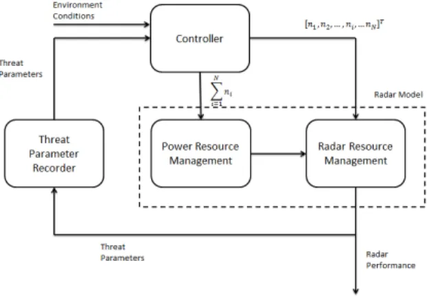
The structure of the radar system is shown in Figure 2. The radar controller decides how many power units should be allocated to the Power Resource Management (PRM) unit and also how those power units are distributed. The PRM allocates the number of power units to the Radar Resource Management (RRM) unit and RRM distributes the power units to different sectors. These power units are utilized to transmit waveforms. This results in detection of threats by the radar model, and it outputs the parameters of the threats. The Threat Parameter Recorder (TPR) records and analyzes the parameters, and then outputs the status of each threat to the controller. The controller takes in this information and generates inputs for the radar model based on the threat parameters and the environmental conditions.
The state machine TPR is the composition of several
Fig. 2. Radar Model Structure.
smaller state machines (STPR). STPR is defined as follows: Suppose the threat needs to be tracked for w time steps before being discriminated,
1) States = {undetected, tracked1, tracked2, ..., tracked(w − 1), discriminated},
2) Inputs={tracking, nottracking}×{losing, notlosing}, 3) Outputs = States,
4) x0 = {undetected},
5) update: States × Inputs → States × Outputs can be decomposed into two functions: nextState : States × Inputs → States and output : States × Inputs → Outputs, which are given as follows: ∀ x(k) ∈ States, ∀ u(k) ∈ Inputs, x(k + 1) = nextState(x(k), u(k)) =
tracked1 ⇐ x(k) = undetected, u(k) = [tracking, :]T tracked m + 1 ⇐ x(k) = tracked m and
u(k) = [:, not losing]T
discriminated ⇐ x(k) = tracked w − 1 and u(k) = [tracking, :]T
undetected ⇐ x(k) 6= discriminated and u(k) = [not tracking, losing]T undetected ⇐ x(k) = undetected and
u(k) = [not tracking, :]T discriminated ⇐ x(k) = discriminated y(k) = output(x(k), u(k)) = x(k + 1)
where tracking and not tracking indicate, respectively, whether a threat is being observed by the radar or not, and losing and not losing indicate, respectively, whether a threat will be lost by radar or not, if it is unobserved at the current time step. Considering there are S threats in this area, then TPR is obtained via side by side composition of S STPR.
The finite state machine PRM is defined as, 1) States = { 0,1,2,3, ..., N }, 2) Inputs = {u ∈ Integers| − N ≤ u ≤ N }, 3) Outputs = States, 4) x0 = 0, 5) update(x(k), u(k)) 7→ (x (k) + u (k) , x (k) + u (k)) ⇐ 0 < x (k) + u (k) < N, (N, N ) ⇐ x (k) + u (k) > N, (0, 0) ⇐ x (k) + u (k) < 0.
The finite state machine RRM is defined as follows: Define A = {a ∈ Integers | 1 ≤ a ≤ M } as the set of indices of sub-areas, and suppose S threats are detected; then B = {(s, as) | as ∈ A, s ∈ Integers and s ≤ S},
so each element in B is a tuple that indicates that the sth
threat is in sub-area as. P(A) is the power set of set A.
1) States = P(A),
2) Inputs = {[n1, n2, ..., ni, ..., nN]T},
3) Outputs = P(B), 4) x0 = ∅,
5) update:∀x(k) ∈ States, and ∀u(k) ∈ Inputs, x(k + 1) = nextState(x(k), u(k)) =
N
[
i=1 & ni>0
{i, i + N, ...i + (ni− 1)N }
where ni indicates each entry of u(k), and
y(k) = output(x(k), u(k)) = {(s, as) ∈ B|as ∈ x(k+1)},
where x(k + 1) is the set of the sub-area indices that are covered by radar waveform, while y(k) is a set of tuples that display the threats located in the sub-areas ∈ x(k + 1). For the example in Figure 1, suppose the index of the
closest northeast sub-area is ”1” and number the sub-areas counterclockwise, then the u(k) to RRM for (a) and (b) are [1 1 1 1]T and [4 0 0 0]T, respectively. For (a) and (b), the elements in x(k + 1) are {1, 2, 3, 4} and {1, 5, 9, 13}, respectively.
C. Radar Controller
The controller is built based on the analysis of each sub-area. It results in the most advantageous sub-areas at each timestep, the advantage being dictated by the cost function. Three factors are considered in the controller design.
When the radar is searching, given a certain RRM input, we assume perfect measurement for all elements in the set x(k). The appearance of a threat in sub-area aq ∈ x(k) has a/
probability Pq, that follows an exponential distribution with
respect to tq, where tq is the time elapsed since aq was last
observed. Therefore, the appearance probability of a threat in those sub-areas Pta is Pq = 1 − e−tq, (7) Pta= 1 − M Y q=1,aq∈x(k)/ (1 − Pq). (8)
When the radar is tracking, the rate at which it collects information after acquisition is modeled as
˙
I = W log2(1 +K
4
r4 ), (9)
where W is a constant determined by the radar, K is determined by the threat, and r indicates the range to the acquired threat [10].
The radar must revisit the same sub-area where a threat is located before the threat exits this area. The revisit deadline is defined as the minimum estimated time that a threat resides in a sub-area. The revisit deadline tdenters the cost function
as a parameter. Let Rv be defined as
Rv= e−td. (10)
For each state, the cost is,
T (x(k), k) = KpPta− KI v X k=1 ˙ Ik+ KRRv (11)
where KP, KI, KR are the weights of each term.
Thus, the transition cost is:
Φ(x(k), u(k), k) = T (u(k), k) − T (x(k), k), (12) with the constraint in Equation (6). Then, at each step, we employ the greedy algorithm to find the input that leads the system to the state with minimum cost value.
Three properties make greed work for our radar modeling. First, the cost function contains all of the information for the current time step and takes into account all of the decisions made at previous time steps. Thus, a given decision for the current time step will change the cost function for the next step. In addition, the threats’ action will also be taken into account by the cost function. Moreover, the states being
unions of the sub-areas that the radars can observe, there is no restriction on movement in the state space and no cost for switching between states.
IV. PROBLEM FORMULATION
The radar resource management problem has been relaxed by certain assumptions in this paper: (1) The motion of the threats and the radar waves are restricted to a horizontal plane; (2) The number of enemy threats is finite and is not capable of overwhelming the defense; (3) There is no electronic warfare, i.e., no jamming of the radars by enemy agents.
Consider a multifunction radar, that is capable of executing both search and track tasks simutaneous via intermittent irradiation. There is a rectangular area of interest A to be defended, with n ships in a linear configuration, separated from each other by a distance of d. There are s1 ballistic
threats and s2 aircraft threats, of different speeds v1 and
v2 from different distances d1 and d2, which are incumbent
upon this fleet of ships. The goal of the defense radar system is to track all these threats until they can be engaged, ensuring zero leakage. The radar has basic tracking range of r0 and a maximum tracking range of rmax. We assume for
this scenario that d ≤ 2rmax. At initial time t0, the threats
are assigned positions at random. They then start moving towards the fleet.
When the ships are under central control, there is perfect communication between the ships, i.e., what is known to one is known to all. When they are decentralized, communication between the ships is absent, i.e., there is no consolidation of the total information available from all the ships.
V. TECHNICAL APPROACH A. Decentralization
In the case of decentralization, there are distinct radar units, modeled identically and controlled by the same con-trol algorithm for each. Moreover, communication between different radar systems is not allowed. Without any commu-nication, each radar system does not know the inputs of the other radars and is only responsible for its own area. B. Centralization
In the case of centralization, the distinct units are inte-grated into one system. We develop rules for composing the state machines and the cost function to build a globally integrated state machine, which is called the Super State Machine (SSM). Consider the formation of three radars shown in Figure 3. The areas monitored by the individual radars overlap. We set a threshold that if one radar’s sub-area overlaps with τ or more of another radar’s sub-sub-area, we can assume that the two sub-areas are the same. Under this assumption, we say that the sub-areas 4A and 2B are the same, as are sub-areas 4B and 2C. These sub-areas are defined as redundant sub-areas. Then we construct a SSM for the whole system. The SSM is composed by parallel composition [7] with one limitation - each super state in the super state space does not contain more than one redundant
sub-area. This prohibits different radars from searching the same sub-area at the same time. If we limit maximum radar power to two units, the super states of the SSM in the given example have the following form:
States = {(C24)A, (C24)B, (C24)C, JA+ JB+ JC}, (13)
where it is not permissible to have 4A and 2B in the same super state and 4B and 2C in the same super state. (C24)A,
(C4
2)B and (C24)C are the two combinations of four radar
areas for the sets {1A, 2A, 3A, 4A}, {1B, 2B, 3B, 4B} and {1C, 2C, 3C, 4C} respectively, and JA, JB, JC are the cost
functions of radar A, radar B, and radar C, respectively. After the SSM is composed, we find the greedy policy by using the same controller with a new cost function, JA+ JB+ JC.
Fig. 3. Radar Formation.
VI. SIMULATION & RESULTS
In the simulation, we use the values of n = 3, d = 424, where n is the number of ships and d is the distance between them. Ballistic threats are initially located very far from the radars, and travel towards the central radar at a constant speed from different directions, while aircraft threats are initially located closer to the central radar and travel towards the radars at a constant speed, slower than that of the missiles, in different directions. The distribution of speeds and initial distances of threats are as follows: v1= 60 units/step, v2= 15 units/step, d1= 1200 units
and d2 = 600 units. In addition, θ = π2 and N = 4 as
defined in Sec. III. Thus, each radar system is capable of allocating four power units among four sectors. Moreover, the threats have to be tracked for at least three time steps before being discriminated.
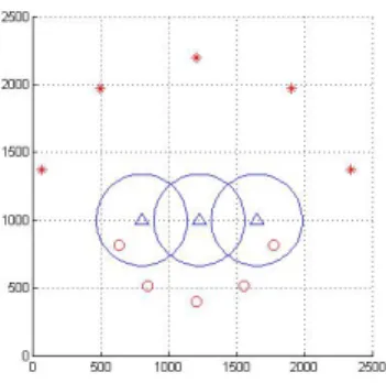
Different numbers of threats are studied to demonstrate the feasibility of the model and controller. Meanwhile, the decentralization and centralization strategies are also com-pared to examine their efficiencies. Considering a case of s1= 5 and s2= 5, the initial configuration of the simulation
is shown in Figure 4. Table I displays the inputs to the central
TABLE I
RRM INPUTS FORCENTRALRADAR
Time Step ¯ 9 10 11 12 13 14 15 16 17 18 19 20 Sector 1 ¯ 0 0 0 0 1 0 0 2 1 1 4 0 Sector 2 ¯ 0 0 0 0 0 4 3 2 0 0 0 4 Sector 3 ¯ 0 4 4 4 3 0 0 0 3 0 0 0 Sector 3 ¯ 4 0 0 0 0 0 1 0 0 3 0 0
Fig. 4. Scenario Configuration: blue triangles indicate the locations of the radars and the blue circles indicate the range of the radar, red stars indicate the ballistic threats and red small circles indicate the aircraft threats.
Fig. 5. An Example of Threat States: ”2” is ”undetected”, ”1” denotes ”tracked” and ”0” is ”discriminated.”
radar from the controller for the example scenario. The table shows how many power units are allocated in each time step, for each transmitting sector.
Figure 5 shows an example of threat states at each time step. Each threat has to be tracked for at least three time steps before being discriminated. There is no transition from a tracked to an undetected state, i.e., the radar does not lose track of a detected threat. At the last time step, all elements of the TPR state are discriminated, which means the radar system has successfully accomplished its task.
The comparison of the simulation results between decen-tralization and cendecen-tralization is shown in Figure 6, Figure 7 and Figure 8. In Figure 6, the total discrimination time indi-cates how many time steps the system takes to discriminate all the threats, i.e., the time-steps range from detecting the first threat to discriminating the last threat. Figure 7 displays the comparison of average missing detection probability Pta
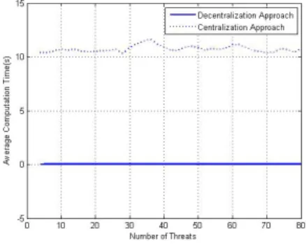
for different cases. The probability value is obtained by Equation (8), which evaluates how likely it is that the radar will miss a threat. Figure 8 shows the average computation time for each time step, which indicates how long it takes to solve for an input at one time step. Altogether, 40 cases are simulated here with s1 = s2 ranging from 1 to 40. The
total number of threats ranges from 2 to 80.
As shown in Figure 6, in all cases analyzed in this paper, the centralization approach can discriminate all the threats in fewer time steps than the decentralization approach.
Fig. 6. Comparison of Total Discrimination Time.
Fig. 7. Comparision of Missing Detection.
As shown in Figure 7, as the number of threats increases, the missing detection probability increases. In other words, the higher the number of threats , the harder it is for the radar systems to achieve zero leakage. Besides, the average value log Pta for the centralization approach is smaller than
that of the decentralization approach. This indicates that the centralization approach is capable of distributing the resources better. Additionally, the difference of missing prob-ability between two cases increases first and then decrease, as the number of threats increases. It indicates that when the number of threats exceeds a certain level, the radar operation is limited by its power limitation. So, missing detection probabilities of both approaches tend to converge to similar value.
However, as shown in Figure 8, the computation time
Fig. 8. Comparison of Average Computation Time.
of the centralization method largely exceeds that of the decentralization method, which means centralization is com-putationally expensive. Therefore, there is a trade off be-tween employing decentralization and centralization for real-time radar control. Moreover, the computation real-time mainly depends on the number of states, which is determined by the total power units. The computation time thus remains relatively flat in each case.
VII. CONCLUSIONS & FUTURE WORK In this paper, a new radar model has been proposed based on a hierarchy of finite state machines. The logical abstraction provided by this model has been shown useful to analyze different possible configurations in a fleet of radars. A control algorithm specific to this radar model has been developed for the purpose of radar resource allocation. This algorithm is based on a cost function that is dependent on the current state and decision and the threat dynamics. An instantaneous minimization of cost is carried out to yield the best decision at each time step. We have compared a centralized control structure with a decentralized (independent) mode of operation, and the results confirm that the centralized approach yields better performance.
VIII. ACKNOWLEDGMENTS
The authors thank Mr. Philippe Kirschen for constructive technical inputs. This research is supported by the Office of Naval Research, U.S Naval Surface Warfare Center, under grant number N00178-12-C-2003.
REFERENCES
[1] N. Visnevski, V. Krishnamurthy, S. Haykin, B. Currie, F. Dilkes, and P. Lavoie. Multi-function radar emitter modelling: A stochastic discrete event system approach. In Proceedings of the 42nd IEEE Conference on Decision and Control, pages 6295–6300, Dec 2003. [2] G. A. Watson and W. D. Blair. Revisit calculation and waveform
control for a multifunction radar. In Proceedings of the 32nd IEEE Conference on Decision and Control, pages 456–461, Dec 1993. [3] S. Ghosh, J. Hansen, R. Rajkumar, and J. Lehoczky. Integrated
resource management and scheduling with multi-resource constraints. In Proceedings of the 25th IEEE International Real-Time Systems Symposium, pages 12–22, Dec 2004.
[4] C. Ting, H. Zishu, and T. Ting. Dwell scheduling algorithm for multifunction phased array radars based on the scheduling gain. Journal of Systems Engineering and Electronics, 19:479–485, June 2008.
[5] J. Seok, J. Zhao, J. Selvakumar, E. Sanjaya, P. T. Kabamba, and A. Girard. Radar resource management: Dynamic programming and dynamic finite state machines. In to be presented in the ECC 2013. [6] S. S. Epp. Discrete mathematics with applications. Cengage Learning,
4th edition, 2010.
[7] C.G. Cassandras and S. Lafortune. Introduction to discrete event systems. Springer, 2nd edition, 2007.
[8] N. A. Lynch and M. R. Tuttled. An introduction to input/output automata. CWI Quarterly, 2:219–246, 1989.
[9] T. H. Cormen, C. E. Leiserson, R. L. Rivest, and C. Stein. Introduction to algorithms. MIT press, 3rd edition, 2001.
[10] B. Hyun, J. Jackson, A. Klesh, A. Girard, and P. Kabamba. Robotic exploration with non-isotropic sensors. In Proceedings of the AIAA GNC Conference, 2009.