doi: 10.1590/0101-7438.2014.034.02.0143
AN EXPERIMENTAL COMPARISON OF BIASED AND UNBIASED RANDOM-KEY GENETIC ALGORITHMS*
Jos´e Fernando Gonc¸alves
1, Mauricio G.C. Resende
2**and Rodrigo F. Toso
3Received June 3, 2014 / Accepted June 14, 2014
ABSTRACT.Random key genetic algorithms are heuristic methods for solving combinatorial optimization problems. They represent solutions as vectors of randomly generated real numbers, the so-called random keys. A deterministic algorithm, called a decoder, takes as input a vector of random keys and associates with it a feasible solution of the combinatorial optimization problem for which an objective value or fitness can be computed. We compare three types of random-key genetic algorithms: the unbiased algorithm of Bean (1994); the biased algorithm of Gonc¸alves and Resende (2010); and a greedy version of Bean’s algorithm on 12 instances from four types of covering problems: general-cost set covering, Steiner triple covering, general-cost setk-covering, and unit-cost covering by pairs. Experiments are run to construct runtime distributions for 36 heuristic/instance pairs. For all pairs of heuristics, we compute probabilities that one heuristic is faster than the other on all 12 instances. The experiments show that, in 11 of the 12 instances, the greedy version of Bean’s algorithm is faster than Bean’s original method and that the biased variant is faster than both variants of Bean’s algorithm.
Keywords: genetic algorithm, biased random-key genetic algorithm, random keys, combinatorial optimiza-tion, heuristics, metaheuristics, experimental algorithms.
1 INTRODUCTION
Genetic algorithms with random keys, or random-key genetic algorithms(RKGA), were first introduced by Bean (1994) for combinatorial optimization problems for which solutions can be represented as a permutation vector, e.g. sequencing and quadratic assignment. In a RKGA, chromosomes are represented as vectors of randomly generated real numbers in the interval [0,1). A deterministic algorithm, called adecoder, takes as input a solution vector and associates with it a feasible solution of the combinatorial optimization problem for which an objective
*Invited paper **Corresponding author
1Universidade do Porto, Rua Dr. Roberto Frias, s/n, 4200-464 Porto, Portugal. E-mail: jfgoncal@fep.up.pt 2AT&T Labs Research, 200 South Laurel Avenue, Room A5-1F34, Middletown, NJ 07748 USA. E-mail: mgcr@research.att.com
value orfitnesscan be computed. In a minimization (resp. maximization) problem, we say that solutions with smaller (resp. larger) objective function values are more fit than those with larger (resp. smaller) values.
A RKGA evolves a population of random-key vectors over a number of iterations, called gener-ations. The initial population is made up ofprealn-vectors of random keys. Each component of the solution vector is generated independently of each other at random in the real interval[0,1). After the fitness of each individual is computed by the decoder in generationk, the population is partitioned into two groups of individuals (see Fig. 1): a small group of pe eliteindividuals,
i.e. those with the best fitness values, and the remaining set of p−penon-eliteindividuals. To
evolve the population, a new generation of individuals must be produced. All elite individual of the population of generationkare copied without modification to the population of generation k+1 (see Fig. 2). Mutation, in genetic algorithms as well as in biology, is key for evolution of the population. RKGAs implement mutation by introducingmutantsinto the population. A mutant is simply a vector of random keys generated in the same way as an element of the initial population. At each generation, a small number (pm) of mutants is introduced into the population
(see Fig. 2). With thepeelite individuals and thepmmutants accounted for in populationk+1,
p−pe−pmadditional individuals need to be produced to complete thepindividuals that make
up the new population. This is done by producing p−pe−pm offspring through the process of
mating or crossover (see Fig. 3).
Figure 1–Population ofpsolutions is partitioned into a smaller set ofpeelite (most fit) solutions and a larger set ofp−penon-elite (least fit) solutions.
Figure 2– All pe elite solutions from populationkare copied unchanged to populationk+1 and pm mutant solutions are generated in populationk+1 as random-key vectors.
Figure 3– To complete populationk+1, p− pe− pm offspring are created by combining a parent selected at random from the elite set of populationkwith a parent selected at random from the non-elite set of populationk. Parents can be selected for mating more than once per generation.
partition (parent B). We say the selection isbiasedsince one parent is always an elite individual. Repetition in the selection of a mate is allowed and therefore an individual can produce more than one offspring in the same generation.Parameterized uniform crossover(Spears & DeJong, 1991) is used to implement mating in both RKGAs and BRKGAs. LetρA>0.5 be the probability that
vectorctakes on the value of thei-th componenta(i)of parent Awith probabilityρAand the
value of thei-th componentb(i) of parent B with probability 1−ρA. In this paper, we also
consider a slight variation of Bean’s algorithm, which we call RKGA∗, where once two parents are selected for mating, the best fit of the two is called parentAwhile the other is parentB.
When the next population is complete, i.e. when it haspindividuals, fitness values are computed by the decoder for all of the newly created random-key vectors and the population is partitioned into elite and non-elite individuals to start a new generation. Figure 4 shows a flow diagram of the BRKGA framework with a clear separation between the problem dependent and problem independent components of the method.
Random-key genetic algorithms search the solution space of the combinatorial optimization problem indirectly by exploring the continuousn-dimensional hypercube, using the decoder to map solutions in the hypercube to solutions in the solution space of the combinatorial optimiza-tion problem where the fitness is evaluated.
As aforementioned, the role of mutants is to help the algorithm escape from local optima. An escape occurs when a locally-optimal elite solution is combined with a mutant and the resulting offspring is better fit than both parents. Another way to avoid getting stuck in local optima is to embed the random-key genetic algorithm in a multi-start strategy. Afterir > 0 generations
without improvement in the fitness of the best solution, the best overall solution is tentatively updated with the best fit solution in the population, the population is discarded and the algorithm is restarted.
To describe a random-key genetic algorithm for a specific combinatorial optimization problem, one needs only to show how solutions are encoded as vectors of random keys and how these vectors are decoded to feasible solutions of the optimization problem. In the next section, we describe random-key genetic algorithms for the four set covering problems problems considered in this paper.
The paper is organized as follows. In Section 2 we describe the four covering problems and in Section 3 we propose random-key genetic algorithms for each problem. Experimental results comparing implementations of RKGA, RKGA∗, and BRKGA for each of the four covering prob-lems are presented in Section 4. We make concluding remarks in Section 5.
2 FOUR SET COVERING PROBLEMS
In this section, we define four set covering problems and propose random-key genetic algorithms for each.
2.1 General-cost set covering
Givennfinite sets P1,P2, . . . ,Pn, let setsI and J be defined asI = ∪nj=1Pj = {1,2, . . . ,m}
andJ= {1, . . . ,n}. Associate a costcj >0 with each element j∈ J. A subsetJ∗⊆Jis called
acoverif∪j∈J∗Pj =I. The cost of the cover is
Figure 4–Flowchart of random-key genetic algorithm with problem independent and problem dependent components.
minimum cost cover. LetAbe the binarym×nmatrix such thatAi,j =1 if and only ifi∈ Pj.
An integer programming formulation for set covering is
min{cx : Ax ≥em, x∈ {0,1}n},
whereem denotes a vector ofmones andx is a binaryn-vector such thatxj = 1 if and only
if j ∈ J∗. The set covering problem has many applications (Vemuganti, 1998) and is NP-hard (Garey & Johnson, 1979).
2.2 Unit-cost set covering
A special case of set covering is wherecj =1, for all j ∈ J. This problem is called the
unit-cost set covering problem and its objective can be thought of as finding a cover of minimum cardinality.
2.3 General-cost setk-covering
Theset k-covering problemis a generalization of the set covering problem, in which each object i ∈ I must be covered by at leastk elements of{P1, . . . ,Pn}. As before, let A be the binary
m×nmatrix such thatAi,j =1 if and only ifi ∈ Pj. An integer programming formulation for
setk-covering is
min{cx : Ax ≥km, x∈ {0,1}n},
Note that the set covering problem (Subsection 2.1) as well as the unit-cost set covering problem (Subsection 2.2) are special cases of setk-covering. In both,k=1 and, furthermore, in unit-cost set coveringcj =1 for all j ∈ J.
2.4 Covering by pairs
Let I = {1,2, . . . ,m}, J = {1,2, . . . ,n}, and associate with each element of j ∈ J a cost cj > 0. For every pair{j,k} ∈ J ×J, with j = k, letπ(j,k)be the subset of elements in I
covered by pair{j,k}. A subsetJ∗⊆ Jis a cover by pairs if
{j,k}∈J∗×J∗
π(j,k)=I.
The cost of J∗is
j∈J∗cj. Theset covering by pairs problemis to find a minimum cost cover
by pairs.
For all j ∈ J, letxj be a binary variable such thatxj =1 if and only if j ∈ J∗. For every pair {j,k} ∈ J×J with j <k, let the continuous variableyj k be such thatyj k ≤xj andyj k ≤xk.
Therefore, ifyj k >0 thenxj =xk =1. Letπ−1(i)denote the set of pairs{j,k} ∈ J×Jthat
coveri∈ I. An integer programming formulation for the covering by pairs problem is
min
j∈J
cjxj
subject to
{j,k}∈π−1(i)
yj k ≥1, ∀i ∈ I,
yj k ≤xj, ∀{j,k} ∈ J×J, (j <k),
yj k ≤xk, ∀{j,k} ∈ J×J, (j <k),
xj = {0,1}, ∀j ∈J,
0≤yj k≤1, ∀{j,k} ∈ J×J, (j <k).
3 RANDOM-KEY GENETIC ALGORITHMS FOR COVERING
Biased random-key genetic algorithms for set covering have been proposed by Resende et al. (2012), Breslau et al. (2011), and Pessoa et al. (2011). These include a BRKGA for the Steiner triple covering problem, a unit-cost set covering problem (Resende et al., 2012), BRKGA heuris-tics for the set covering and setk-covering problems (Pessoa et al., 2011), and a BRKGA for set covering by pairs (Breslau et al., 2011). We review these heuristics in the remainder of this section.
The random-key genetic algorithms for the set covering problems of Section 2 that we describe in this section all encode solutions as a|J|-vectorXof random keys. The j-th keyXjcorresponds
to the j-th element of setJ.
Xj > 1/2. If J∗ is a feasible cover, then step 2 is skipped. Otherwise, in step 2, a greedy
algorithm is used to construct a valid cover starting fromJ∗. Later in this section, we describe these greedy algorithms. Finally, in step 3, a local improvement procedure is applied to the cover. Later in this section, we describe the different local improvement procedures.
The decoder not only returns the cover J∗but also modifies the vector of random keysXsuch
that it decodes directly intoJ∗with the application of only the first phase of the decoder. To do this we resetXas follows:
Xj =
⎧ ⎪ ⎪ ⎪ ⎪ ⎪ ⎨
⎪ ⎪ ⎪ ⎪ ⎪ ⎩
Xj if Xj ≥0.5 and j ∈ J∗
1−Xj if Xj <0.5 and j∈ J∗
Xj if Xj <0.5 and j∈ J∗
1−Xj if Xj ≥0.5 and j ∈J∗.
3.1 Greedy algorithms
We use two greedy algorithms. The first is for setk-covering and its special cases, set covering and unit-cost set covering. The second one is for covering by pairs.
3.1.1 Greedy algorithm for setk-covering
A greedy algorithm for set covering (Johnson, 1974) starts from the partial cover J∗ defined byX. This greedy algorithm proceeds as follows. WhileJ∗is not a valid cover, add toJ∗the
smallest index j ∈ J\ J∗for which the inclusion of j inJ∗corresponds to the minimum ratio πj of costcj to number of yet-uncovered elements ofIthat become covered with the inclusion
of j in J∗. For the special case of unit-cost set covering, this reduces to adding the smallest index j ∈ J\J∗for which the inclusion of jinJ∗maximizes the numberπj of yet-uncovered
elements ofI that become covered with the inclusion of j in J∗. In this iterative process, we use a binary heap to store theπj values of unused columns, allowing us to retrieve a column
j with largestπj value in O(logm)-time and update theπ values of the remaining columns in
O(logn)-time after column jis added to the solution.
3.1.2 Greedy algorithm for unit-cost covering by pairs
A greedy algorithm for unit-cost covering by pairs is proposed in Breslau et al. (2011). It starts with set J∗defined byX. Then, as long asJ∗is not a valid cover, find an element j ∈ J\J∗
such thatJ∗∪{f}covers a maximum number of yet-uncovered elements ofI. Ties are broken by the index of element j. If the number of yet-uncovered elements ofI that become covered is at least one, addjtoJ∗. Otherwise, find a pair of{j1,j2} ⊆ J\J∗such thatJ∗∪ {j1}∪ {j2}covers
a maximum number of yet-uncovered elements inI. Ties are broken first by the index of j1, then
by the index of j2. If such a pair does not exist, then the problem is infeasible. Otherwise, add
3.2 Local improvement procedures
Given a cover J∗, the local improvement procedure attempts to make elementary modifications to the cover with the objective of reducing its cost. We use two types of local improvement pro-cedures: greedy uncoverand1-opt. In the decoder for setk-covering we apply greedy uncover, followed by 1-opt, followed by greedy uncover if necessary. In the special case of unit-cost set covering only greedy uncover is used. The decoder implemented for set covering by pairs does not make use of any local improvement procedure. Instead, greedy uncover is applied to each elite solution after the iterations of the genetic algorithm end. In the experiments described in Section 4, this local improvement is not activated.
3.2.1 Greedy uncover
Given a cover J∗,greedy uncoverattempts to remove superfluous elements of J∗, i.e. elements j∈ J∗such that J∗\ {j}is a cover. This is done by scanning the elements j ∈ J∗in decreasing order of costcj, removing those elements that are superfluous.
3.2.2 1-Opt
Given a cover J∗,1-Optattempts to find an element j ∈ J∗and another elementi ∈ J∗such thatci <cj andJ∗\ {j} ∪ {i}is a cover. If such a pair is found,ireplaces jinJ∗. This is done
by scanning the elements j ∈ J∗in decreasing order of costcj, searching for an elementi ∈ J∗
that covers all elements ofIleft uncovered with the removal of each j∈ J∗.
4 COMPUTATIONAL EXPERIMENTS
We report in this section computational results with the two variants of random-key genetic algorithms (the biased variant – BRKGA – and Bean’s unbiased variant – RKGA) of Section 1 as well as a variant of Bean’s algorithm which we shall refer to as RKGA*. Like Bean’s RKGA, RKGA* selects both parents at random from the entire population. This is unlike a BRKGA, where one parent is always selected from the elite partition of the population and the other from the non-elite partition. Unlike Bean’s algorithm, a RKGA* assigns the best fit of both parents as parent Aand the other asparent Bfor crossover. Ties are broken by rank in the sorted population. RKGA assigns the selected parents to the roles ofparent Aandparent Bat random.
Our goal in these experiments is to compare these three types of heuristics on different problem instances and show that the BRKGA is the most effective of the three.
scp48-7 of Pessoa et al. (2013). For unit-cost covering by pairs, we consider instances
n558-i0-m558-b140,n220-i0-m220-b220, andn190-i9-m190-b95of Breslau et al. (2011).
The experiment consists in running the three variants (BRKGA, RKGA, and RKGA*) 100 times on each of the 12 instances. Therefore, the genetic algorithms are run a total of 3600 times. Each run is independent of the other and stops when a solution with cost at least as good as a given target solution value is found. The objective of these runs is to derive empirical runtime distri-butions, or time-to-target (TTT) plots (Aiex et al., 2007) for each of the 36 instance/variant pairs and then estimate the probabilities that a variant is faster than each of the other two, using the iterative method proposed in Ribeiro et al. (2012). This way, the three variants can be compared on each instance.
Table 1 lists the instances, their dimensions, the values of the target solutions used in the experi-ments, and the best solution known to date.
Table 1–Test instances used in the computational experiments. For each instances, the table lists its class, name, dimensions, value of the target solution used in the experiments, and the value of the best solution known to date.
Problem class Instance name m n k Triples Target BKS
General set covering scp41 200 1000 1 – 429 429
scp51 200 2000 1 – 253 253
scpa1 300 3000 1 – 253 253
Steiner triple covering stn135 3015 135 1 – 103 103
stn243 9801 243 1 – 198 198
stn405 27270 405 1 – 339 335
Setk-covering scp41-2 200 1000 2 – 1148 1148
scp45-11 200 1000 11 – 188856 188856
scp48-7 200 1000 7 – 8421 8421
Covering by pairs n558-i0-m558-b140 558 140 1 1,301,314 55 50
n220-i0-m220-b220 220 220 1 289,657 62 62
n190-i9-m190-b95 190 95 1 173,030 37 37
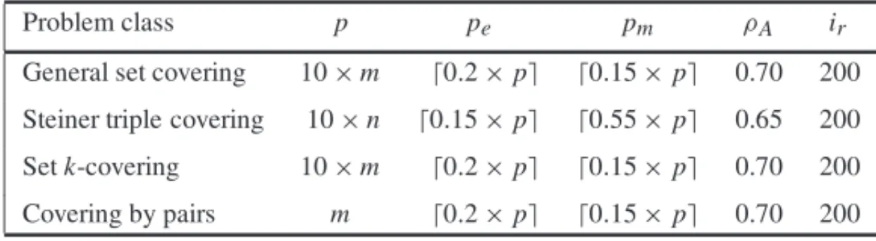
Table 2–Parameter settings used in the computational experiments. For each problem class, the table lists its name and the following parameters: size of population (p), size of elite partition (pe), size of mutant set (pm), inheritance probability (ρA), and number of iterations without improvement of incumbent that triggers a restart (ir).
Problem class p pe pm ρA ir
General set covering 10×m ⌈0.2×p⌉ ⌈0.15×p⌉ 0.70 200 Steiner triple covering 10×n ⌈0.15×p⌉ ⌈0.55×p⌉ 0.65 200
Setk-covering 10×m ⌈0.2×p⌉ ⌈0.15×p⌉ 0.70 200 Covering by pairs m ⌈0.2×p⌉ ⌈0.15×p⌉ 0.70 200
The goal of the experiment is to derive runtime distributions for the three heuristics on a set of 12 instances from the four problem classes. Runtime distributions, or time-to-target plots (Aiex et al., 2007), are useful tools for comparing running times of stochastic search algorithms. Since the experiments involve running the algorithms 3600 times, with some very long runs, we distributed the experiment over several heterogeneous computers. Since CPU speeds vary among the computers used for the experiment, instead of producing runtime distributions directly, we first derive computer-independent iteration count distributions and use them to subsequently derive runtime distributions. To do this, we multiple iteration counts for each heuristic/instance pair by their corresponding mean running time per iteration. Mean running times per iteration of each heuristic/instance pair are estimated on an 8-thread computer with an Intel Core i7-2760QM CPU running at 2.40GHz. On the 12 instances, we ran each heuristic independently 10 times for 100 generations and recorded the average running (user) time. User time is the sum of all running times on all threads and corresponds to the running time on a single processor. These times are listed in Table 3.
Figures 5 –16 show iteration count distributions for the three heuristics on each of the 12 problem instances that make up the experiment. Suppose that for a given variant, all 100 runs find a solution at least as good as the target and lett1,t2, . . . ,t100be the corresponding iteration counts
sorted from smallest to largest. Each iteration count distribution plot shows the pairs of points
{t1, .5/100},{t2,1.5/100}, . . . ,{t100,99.5/100},
connected sequentially by lines. For each heuristic/instance pair and target solution value, the point {ti, (i −0.5)/100}on the plot indicates that the probability that the heuristic will find
a solution for the instance with cost at least as good as the target solution value in at mostti
iterations is(i−0.5)/100, fori=1, . . . ,100.
For each heuristic/instance pair, let τ denote the average CPU time for one iteration of the heuristic on the instance. Then a runtime distribution plot can be derived from an iteration count distribution plot with the pairs of points
Table 3–Average CPU time per 100 generations for each problem and each algo-rithm. For each instance, the table list the CPU times (in seconds on an Intel Core i7-2760QM CPU at 2.40GHz) for 100 generations of heuristics BRKGA, RKGA, and RKGA*. Averages were computed over 10 independent runs of each heuristic.
Instance name BRKGA RKGA RKGA*
scp41 21.01 24.71 22.67
scp51 29.64 34.20 31.57
scpa1 68.30 82.82 77.73
stn135 17.61 18.05 18.43
stn243 134.67 137.99 137.20
stn405 769.87 777.37 773.80
scp41-2 43.28 50.76 47.08
scp45-11 398.94 412.35 404.60
scp48-7 211.79 231.89 218.87
n558-i0-m558-b140 318.36 426.89 386.53
n220-i0-m220-b220 34.62 43.14 39.81
n190-i9-m190-b95 12.55 15.95 14.26
For each heuristic/instance pair and target solution value, the point{τ ×ti, (i −0.5)/100}on
the plot indicates that the probability that the heuristic will find a solution for the instance with cost at least as good as the target solution value in at most timeτ ×ti is(i −0.5)/100, for
i=1, . . . ,100.
Iteration count distributions are a useful graphical tool to compare algorithms on a given in-stance. Consider, for example, the plots in Figure 5 which shows iteration count distributions for BRKGA, RKGA*, and RKGA for general-cost set covering instancescp41using the op-timal solution of 429 as the target solution. The plots in this figure clearly show an ordering of the heuristics with respect to the number of iterations needed to find an optimal solution. For example the probabilities that BRKGA, RKGA*, and RKGA will find n optimal solution in at most 2000 iterations are, respectively, 83.5%, 58.5%, and 49.5%. Similarly, with a probability of 60.5% the heuristics BRKGA, RKGA*, and RKGA will find an optimal solution in at most 1076, 2139, and 2715 iterations.
0 0.1 0.2 0.3 0.4 0.5 0.6 0.7 0.8 0.9 1
0 2000 4000 6000 8000 10000 12000 14000 16000
cumulative probability
iterations to target solution
BRKGA RKGA* RKGA
Figure 5–Iteration count distributions for BRKGA, RKGA*, and RKGA on instancescp41with target solution 429.
To produce runtime distributions we would ideally run the experiments on the same machine. Since for these experiments this was not practical, we estimate runtime distributions on a machine by computing the average time per iteration of the heuristic on the instance on the machine and then multiply the entries of the iteration count distributions by the corresponding average time per iteration.
Visual examination of time-to-target plots usually allow easy ranking of heuristics. However, we may wish to quantify these observations. To do this we rely on the iterative method described in Ribeiro et al. (2012). Their iterative method takes as input two sets ofktime-to-target values {ta1,ta2, . . . ,tak}and{tb1,tb2, . . . ,tbk}, drawn from unknown probability distributions, correspond-ing to, respectively, heuristicsa andb and estimates Pr(ta ≤ tb), the probability thatta ≤ tb,
whereta andtbare the random variables time-to-target solution of heuristicsa andb,
respec-tively. Their algorithm iterates until the error is less than 0.001. A perl language script of their method is described in Ribeiro & Rosseti (2013). Applying their program to the sets of time-to-target values collected in the experiment, we compute Pr(tBRKGA ≤tRKGA), Pr(tBRKGA≤tRKGA∗), and Pr(tRKGA∗≤tRKGA) for all 12 instances. These values are shown in Table 4.
We make the following remarks about the experiment.
random-Table 4–Probability that time-to-target solution of BRKGA (tBRKGA) will be less than that of RKGA (tRKGA) and RKGA* (tRKGA∗) and probability that time-to-target solution of RKGA* will be less than that of RKGA on an Intel Core i7-2760QM CPU at 2.40GHz. Computed for empirical runtime distri-butions of the three heuristics using the iterative method of Ribeiro et al. (2012).
Instance name Pr(tBRKGA≤tRKGA) Pr(tBRKGA≤tRKGA∗) Pr(tRKGA∗ ≤tRKGA)
scp41 0.740 0.652 0.588
scp51 0.999 0.960 0.943
scpa1 0.733 0.643 0.642
stn135 0.485 0.496 0.489
stn243 0.864 0.730 0.768
stn405 0.917 0.721 0.859
scp41-2 0.999 0.975 0.975
scp45-11 0.881 0.547 0.854
scp48-7 0.847 0.591 0.797
n558-i0-m558-b140 0.892 0.743 0.754
n220-i0-m220-b220 0.883 0.735 0.734
n190-i9-m190-b95 0.841 0.728 0.701
key genetic algorithm (Bean, 1994) – RKGA, and a slightly modified variant of RKGA – RKGA*, on four classes of combinatorial optimization problems: general-cost set cover-ing, Steiner triple covercover-ing, general-cost setk-covering, and unit-cost covering by pairs. For each of the four problem classes, runtime distributions were generated for each of the three heuristics on three problem instances.
• Since the number of runs required to carried out the experiment was large (3600) and many runs were lengthy, we distributed them on four multi-core linux computers and generated iteration count distributions for all 36 heuristic/instance pairs. Each iteration count distri-bution was produced running the particular heuristic on the instance 100 times, each using a different initial seed as input for the random number generator.
• Of the 12 instances, a target solution value equal to the best known solution was used on 10 instances while on two (stn405andn558-i0-m558-b140) larger values were used. The best known solution to this date for stn405is 435 and we used a target solution value of 439 while for n558-i0-m558-b140the best known solution is 50 and we used 55. This was done since Bean’s algorithm did not find the best known solutions for these instances after repeated attempts.
0 0.1 0.2 0.3 0.4 0.5 0.6 0.7 0.8 0.9 1
4 6 8 10 12 14 16 18 20 22
cumulative probability
iterations to target solution
BRKGA RKGA* RKGA
Figure 6–Iteration count distributions for BRKGA, RKGA*, and RKGA on instancescp51with target solution 253.
tion. On all instances BRKGA was the fastest per iteration of the three heuristics while on all but one instance (stn135), RKGA* was faster per iteration than RKGA. BRKGA was as high as 34% faster than RKGA (onn558-i0-m558-b140) to as low as 1% faster (on stn405) while it was as high as 21% faster than RKGA* (onn558-i0-m558-b140) to as low as 0.5% faster (onstn405). These differences in running times per iteration can be explained by the fact that the incomplete greedy algorithms as well as the local searches implemented in the decoders take longer to converge when starting from random vectors, i.e. vectors containing keys mostly from mutants (recent descendents of mutants). This behavior has been also observed in GRASP heuristics where variants with restricted candidate list (RCL) parameters leading to more random constructions usually take longer than those with more greedy constructions (Resende & Ribeiro, 2010). Of the three vari-ants, RKGA is the most random, while BRKGA is the least. The exception is in the Steiner triple covering class where the algorithms have parameter settings that make them near equally random. In that class, we observe the most similar running times per iteration.
0 0.1 0.2 0.3 0.4 0.5 0.6 0.7 0.8 0.9 1
0 500 1000 1500 2000 2500 3000 3500 4000 4500 5000
cumulative probability
iterations to target solution
BRKGA RKGA* RKGA
Figure 7–Iteration count distributions for BRKGA, RKGA*, and RKGA on instancescpa1with target solution 253.
0 0.1 0.2 0.3 0.4 0.5 0.6 0.7 0.8 0.9 1
0 20000 40000 60000 80000 100000 120000 140000
cumulative probability
iterations to target solution
BRKGA RKGA* RKGA
0 0.1 0.2 0.3 0.4 0.5 0.6 0.7 0.8 0.9 1
0 500 1000 1500 2000 2500 3000 3500 4000 4500
cumulative probability
iterations to target solution
BRKGA RKGA* RKGA
Figure 9–Iteration count distributions for BRKGA, RKGA*, and RKGA on instancestn243with target solution 198.
0 0.1 0.2 0.3 0.4 0.5 0.6 0.7 0.8 0.9 1
0 1000 2000 3000 4000 5000 6000 7000 8000
cumulative probability
iterations to target solution
BRKGA RKGA* RKGA
0 0.1 0.2 0.3 0.4 0.5 0.6 0.7 0.8 0.9 1
0 10 20 30 40 50 60 70
cumulative probability
iterations to target solution
BRKGA RKGA* RKGA
Figure 11–Iteration count distributions for BRKGA, RKGA*, and RKGA on instancescp41-2with target solution 1148.
0 0.1 0.2 0.3 0.4 0.5 0.6 0.7 0.8 0.9 1
0 50000 100000 150000 200000 250000 300000 350000
cumulative probability
iterations to target solution
BRKGA RKGA RKGA
0 0.1 0.2 0.3 0.4 0.5 0.6 0.7 0.8 0.9 1
0 100000 200000 300000 400000 500000 600000
cumulative probability
iterations to target solution
BRKGA RKGA* RKGA
Figure 13–Iteration count distributions for BRKGA, RKGA*, and RKGA on instancescp48-7with target solution 8421.
0 0.1 0.2 0.3 0.4 0.5 0.6 0.7 0.8 0.9 1
0 5000 10000 15000 20000 25000 30000 35000 40000
cumulative probability
iterations to target solution
BRKGA RKGA* RKGA
Figure 14 – Iteration count distributions for BRKGA, RKGA*, and RKGA on instance
0 0.1 0.2 0.3 0.4 0.5 0.6 0.7 0.8 0.9 1
0 5000 10000 15000 20000 25000 30000
cumulative probability
iterations to target solution
BRKGA RKGA* RKGA
Figure 15 – Iteration count distributions for BRKGA, RKGA*, and RKGA on instance
n220-i0-m220-b220with target solution 62.
other problems. The less random parameter settings simply did not result in BRKGAs that were as effective as the more random variant. With respect to stn135, it appears that even more randomness results in improved performance. Of the three heuristics, the most random is RKGA while the least random is BRKGA.
• Visual inspection of Figures 5 to 16 shows a clear domination of BRKGA over RKGA, with the exception of instancestn135. This is backed up by the probabilities shown in Table 4, where 0.733≤Pr(tBRKGA ≤tRKGA)≤0.999 for all but instancestn135where
Pr(tBRKGA ≤tRKGA)=0.485.
• Visual inspection of Figures 5 to 16 shows a clear domination of BRKGA over RKGA*, with the exception of instancesstn135andscp45-11. This is backed up by the prob-abilities shown in Table 4, where 0.591 ≤ Pr(tBRKGA ≤ tRKGA∗) ≤ 0.975 for all but instances instancesstn135andscp45-11, where Pr(tBRKGA ≤ tRKGA∗) =0.496 and
0.547, respectively.
• Visual inspection of Figures 5 to 16 shows a clear domination of RKGA* over RKGA, with the exception of instancescp41. This is backed up by the probabilities shown in Table 4, where 0.588 ≤ Pr(tBRKGA ≤ tRKGA) ≤ 0.975 for all but instancesscp41and
0 0.1 0.2 0.3 0.4 0.5 0.6 0.7 0.8 0.9 1
0 1000 2000 3000 4000 5000 6000 7000
cumulative probability
iterations to target solution
BRKGA RKGA* RKGA
Figure 16 – Iteration count distributions for BRKGA, RKGA*, and RKGA on instance
n190-i9-m190-b95with target solution 37.
5 CONCLUDING REMARKS
This paper studies runtime distributions for three types of random-key genetic algorithms: the algorithm of Bean (1994) – RKGA, a slight modification of Bean’s algorithm in which the best fit of the two parents selected for mating has higher probability of passing along its keys to its offspring – RKGA*, and the biased random-key genetic algorithm of Gonc¸alves & Resende (2011) – BRKGA. We use the methodology described in Aiex et al. (2007) to generate plots of iteration count distributions for BRKGA, RKGA*, and RKGA on problem instances from four classes of set covering problems: general-cost covering, Steiner triple covering, general cost set k-covering, and unit-cost covering by pairs. In each class, the experiment considers three instances. On each, the heuristics are run 100 times, independently, and stop when a given target solution value (in most cases the best known solution value) is found.
To obtain runtime distributions from the iteration count distributions we multiply iteration counts for each algorithm/instance pair by the corresponding average time per iteration obtained by running all algorithm/instance pairs 10 times for 100 iterations on the same computer.
We conclude that Bean’s algorithm (RKGA) can be improved by simply making the best fit of the two parents chosen for mating have a higher probability of passing along its keys to it offspring than the other parent. The resulting algorithm is denoted RKGA*. For 11 of the 12 instances Pr(tRKGA∗ ≤tRKGA)≥0.588, wheretAis the random variable time-to-target solution
of heuristicA. In 9 of the 12 instances Pr(tRKGA∗ ≤ tRKGA) ≥ 0.7. In 4 of the 12 instances
Pr(tRKGA∗ ≤ tRKGA) ≥ 0.854. In 2 of the 12 instances Pr(tRKGA∗ ≤ tRKGA) ≥ 0.943. The
biased random-key genetic algorithm (BRKGA) does even better. In 11 of the 12 instances Pr(tBRKGA ≤ tRKGA) ≥ 0.733. In 9 of the 12 instances Pr(tBRKGA ≤ tRKGA) ≥ 0.841. In 3
of the 12 instances Pr(tBRKGA ≤ tRKGA) ≥ 0.917. Despite the fact that BRKGA has to order
the population by fitness at each iteration, in addition to the same work done by RKGA and RKGA*, it is still faster per iteration, on average, than both RKGA and RKGA*. This is mainly due to the fact that it is not as random as RKGA and RKGA*. Combining time per iteration with number of iterations shows that BRKGA is faster than RKGA*, too. In 11 of the 12 instances Pr(tBRKGA ≤ tRKGA∗)≥0.547. In 9 of the 12 instances Pr(tBRKGA ≤ tRKGA∗)≥0.643. In 7 of the 12 instances Pr(tBRKGA ≤tRKGA∗)≥0.721. In 2 of the 12 instances Pr(tBRKGA ≤tRKGA∗)≥ 0.96.
Randomness is not always bad. On the Steiner triple covering instances, where the fitness land-scapes are flat, it pays off to be more random. In fact, for the Steiner triple covering class, the parameter setting of BRKGA was more random than usual, with pm = ⌈.55p⌉instead of the
usual⌈.15p⌉andρA=0.65 instead of the usual 0.7. BRKGA was faster than both RKGA and
RKGA* on bothstn243andstn405. Onstn135, however, both RKGA and RKGA* were slightly faster than BRKGA, with Pr(tRKGA∗ ≤ tBRKGA) = 0.504 and Pr(tRKGA ≤ tBRKGA)=
0.515.
Though we have confined this study only to set covering problems, we have observed that the described relative performances of the three variants occurs on most, if not all, other problems we have tackled with biased random-key genetic algorithms (Gonc¸alves & Resende, 2011).
ACKNOWLEDGMENT
This research has been partially supported by funds granted by the ERDF through the Pro-gramme COMPETE and by the Portuguese Government through FCT – Foundation for Science and Technology, project PTDC/EGE-GES/117692/2010.
REFERENCES
[1] AIEXRM, RESENDEMGC & RIBEIROCC. 2007. TTTPLOTS: A perl program to create time-to-target plots.Optimization Letters,1: 355–366.
[2] BEANJC. 1994. Genetic algorithms and random keys for sequencing and optimization.ORSA J. on Computing,6: 154–160.
[4] BRESLAUL, DIAKONIKOLASI, DUFFIELDN, GUY, HAJIAGHAYIM, JOHNSONDS, RESENDE MGC & SENS. 2011. Disjoint-path facility location: Theory and practice. In:ALENEX 2011: Work-shop on algorithm engineering and experiments, January.
[5] GAREY MR & JOHNSONDS. 1979. Computers and intractability. A guide to the theory of NP-completeness. W.H. Freeman and Company, San Francisco, California.
[6] GONC¸ALVESJF & RESENDEMGC. 2011. Biased random-key genetic algorithms for combinatorial optimization.J. of Heuristics,17: 487–525.
[7] JOHNSONDS. 1974. Approximation algorithms for combinatorial problems.Journal of Computer and System Sciences,9: 256–278.
[8] PESSOALS, RESENDEMGC & TOSO RF. 2011. Biased random-key genetic algorithms for set
k-covering. Technical report, AT&T Labs Research, Florham Park, New Jersey.
[9] PESSOALS, RESENDEMGC & RIBEIROCC. 2013. A hybrid Lagrangean heuristic with GRASP and path relinking for setk-covering.Computers and Operations Research,40: 3132–3146.
[10] RESENDEMGC & RIBEIROCC. 2010. Greedy randomized adaptive search procedures: Advances and applications. In: Gendreau and J.-Y. Potvin, editors, Handbook of Metaheuristics, pages 281–317. Springer, 2nd edition.
[11] RESENDEMGC, TOSORF, GONC¸ALVESJF & SILVARMA. 2012. A biased random-key genetic algorithm for the Steiner triple covering problem.Optimization Letters,6: 605–619.
[12] RIBEIROCC & ROSSETII. 2013.tttplots-compare: A perl program to compare time-to-target plots or general runtime distributions of randomized algorithms. Technical report, Department of Computer Science, Universidade Federal Fluminense, Rua Passo da P´atria 156, Niter´oi, RJ 24210-240, Brazil.
[13] RIBEIROCC, ROSSETII & VALLEJOSR. 2012. Exploiting run time distributions to compare se-quential and parallel stochastic local search algorithms.J. of Global Optimization,54: 405–429.
[14] SPEARSWM & DEJONGKA. 1991. On the virtues of parameterized uniform crossover. In: Pro-ceedings of the Fourth International Conference on Genetic Algorithms, pages 230–236.
[15] TOSORF & RESENDEMGC. 2014. A C++ application programming interface for biased random-key genetic algorithms.Optimization Methods and Software. doi: 10.1080/10556788.2014.890197.
[16] VEMUGANTI RR. 1998. Applications of set covering, set packing and set partitioning models: A survey. In: D-Z. DU & P.M. PARDALOS, editors, Handbook of Combinatorial Optimization,