doi: 10.1590/0101-7438.2018.038.01.0031
STEPWISE SELECTION OF VARIABLES IN DEA USING CONTRIBUTION LOADS
Fernando Fernandez-Palacin, Maria Auxiliadora Lopez-Sanchez
and Manuel Mu˜noz-M´arquez*
Received March 14, 2017 / Accepted September 27, 2017
ABSTRACT.In this paper, we propose a new methodology for variable selection in Data Envelopment Analysis (DEA). The methodology is based on an internal measure which evaluates the contribution of each variable in the calculation of the efficiency scores of DMUs. In order to apply the proposed method, an algorithm, known as “ADEA”, was developed and implemented in R. Step by step, the algorithm maximizes the load of the variable (input or output) which contribute least to the calculation of the efficiency scores, redistributing the weights of the variables without altering the efficiency scores of the DMUs. Once the weights have been redistributed, if the lower contribution does not reach a previously given critical value, a variable with minimum contribution will be removed from the model and, as a result, the DEA will be solved again. The algorithm will stop when all variables reach a given contribution load to the DEA or until no more variables can be removed. In this way and contrary to what is usual, the algorithm provides a clear stop rule. In both cases, the efficiencies obtained from the DEA will be considered suitable and rightly interpreted in terms of the remaining variables, indicating the load themselves; moreover, the algorithm will provide a sequence of alternative nested models – potential solutions – that could be evaluated according to external criterion. To illustrate the procedure, we have applied the methodology proposed to obtain a research ranking of Spanish public universities. In this case, at each step of the algorithm, the critical value is obtained based on a simulation study.
Keywords: DEA, linear programming, variable selection, measure variable contribution.
1 INTRODUCTION
Data Envelopment Analysis (DEA) is a methodology introduced by Charnes, Cooper and Rodes in [14], that it is used to compare the efficiencies of a set of homogeneous units (DMUs) that produces several outputs from the same set of inputs. This methodology has become very popular in several fields of mathematics and management science, including finance, banking, education, healthcare, . . . For each DMU, the DEA analysis does not only provide an efficiency score, but it
*Corresponding author.
also provides a peer set. The peer set can be used to guide those who are involved in the decision making process, leading to an optimal DMUs performance.
DEA is a non parametric method that builds and estimates the technological frontier as the region defined by the efficiency units. For each DMU, the DEA considers two sets of weights, one set for inputs and another for outputs, obtaining the efficiency scores of the DMUs from the optimization of the ratio between a combination of both sets of variables. The weights are selected in the most favourable way for the unit that has been evaluated. Thus, the initial set of variables, inputs and outputs, can lead to different ways of measuring the efficiency, so it is very important that the set is chosen correctly. Sexton [49], Smith [47] and Dyson [18] get different results regarding the sensitivity in the calculation of efficiencies dependent on variable selection.
As the selection of the variables to be included in the analysis is usually made by the decision makers and politicians, the researchers assume, a priori, that the selection is a correct one. This means that, generally, a very small attention is devoted to the selection of variables as shown in Cook & Zhu [17]. But taking into account that efficiency is measured using the variables included in the model, the inclusion in it of inappropriate or irrelevant variables may cause bias in the results. Thus, the selection of the set of variables becomes an important task.
As will be described below, the usual methods of selection of variables in DEA mainly try to preserve the efficiency scores of the initial model, so the bias remains hidden for the method. We propose a new measure that can detect such bias in the selection of variables. To resolve the procedures involved in the proposed methodology, we have developed a package in R, called aBenchmarking, which will be available in cran [43]. Currently, an interactive online application is available athttp://knuth.uca.es/DEA.
In order to apply the proposed methodology, we will obtain the efficiencies of the research activ-ity of Spanish public universities. For this purpose, we will use the same source of data used by the authors of the “Ranking 2013 de investigaci´on de las universidades p´ublicas espa˜nolas” [12], popularly known as Granada ranking. This is one of the most important rankings of Spanish uni-versities. The Granada ranking includes two rankings, one of production and one of productivity, taking into account in the latter case the human resources that each university has to obtain its scientific production. The ranking of Granada is elaborated since year 2009 with annual period-icity, see [8, 9, 10, 11, 12]. One of the objectives that we intend to address in future works, as application of the methodology proposed in this paper, is to compare the productivity results of the Granada ranking with the efficiencies obtained from a DEA model oriented to output.
2 LITERATURE REVIEW
The usual procedure of dealing with the aforementioned problem is to apply a backward/forward variable selection method, starting with a full model and dropping variables in an stepwise algo-rithm. Many of these methods are taken from classical statistics procedures. Jenkins & Anderson in [31], use the partial correlation coefficient to preserve a subset of variables that retain most of the original information. Simar & Wilson in [51] use bootstrap methods to include signifi-cant variables in a forward selection procedure. Ruggiero in [44] proposes a forward selection method in which, at each step, the entry criterion is based on the correlation of the candidate entry variables with the efficiencies obtained in the current model. Other authors, such as Wag-ner & Shimshak [56] propose similar stepwise methods but using as a criterion the minimization of the change in average efficiency scores. Norman & Stoker in [40] and Sigala et al., in [45], have proposed forward procedures taking into account the correlation between the variables not included in the model and the efficiency scores. Ueda & Hoshiai in [54] and Adler & Golany in [2, 3], developed, independently, a method based on replacing the original variables with the principal component analysis, removing the effect of the redundancy of information.
A different point of view is proposed in other papers. Pastor et al., in [42], suggest a forward model based on the marginal impact of a variable (input-output), which is estimated through an efficiency contribution measure (ECM).
Other method for the selection of variables is the one proposed by Lins & Moreira [35] that starts from a model with only one input and output, the most correlated. From here on, they include that variable that causes higher average efficiency in the DEA, regardless of how many DMUs are efficient. Soares de Mello & others [46] use a convex combination of two indicators, to take into account both the average efficiency and the number of DMUs. To give equal importance to the indicators, the coefficients of the combination are the same, unless there are reasons for not being. A variant of this method is proposed by Senra & others [1], since they begin with the combination of variables that present greater value in the previous combination, although those models that have less variables will have a lower efficiency value since it is known that by increasing the number of variables in DEA increases the average efficiency.
Madhanagopal & Chandrasekaran in [38] first sort the variables by their relevance using a ge-netic algorithm, and then they apply the method proposed by Pastor. Fanchon in [23] suggests a methodology to identify the optimal number of variables, evaluating the contribution of these in the construction of the efficiency frontier. Morita & Avkiran in [37] propose an input/output selection method that uses diagonal layout experiments to find an optimal combination. Sharma & Jin in [52] evaluated the importance of each variable using a Kruskal-Wallis test.
Finally, Sirvent et al., in [48], Adler & Yazhemsky in [6] and Nataraja & Johnson in [39], make a comparative analysis of some of the variable selection techniques proposed in the literature.
Table 1–Main contributions to the selection of variables in DEA.
Methods based on efficiency Classical statistics methods 1982 Lewin, Morey & Cook 1989 Roll, Golany & Seroussy Norman & Stoker 1991
Banker 1996
1997 Ueda & Hoshiai Lins & Moreira 1999
Simar & Wilson 2001 Adler & Golany Pastor, Ruiz & Sirvent 2002
Fanchon 2003 Jenkins & Anderson Sigala
Soares de Mello & others
2004
Ruggiero 2005 Senra & others
Wagner & Shimshak
2007
Gonz´alez-Araya & Vald´es Valenzuela 2009
2011 Kao, Lu & Chiu 2012 Bian
2013 Lin & Chiu Sharma & Yu 2015
Jitthavech Subramanyam
2016
3 METHOD FOR SELECTING VARIABLES BASED ON CONTRIBUTIONS
Our methodology proposes to establish a process of selection of variables that takes into account the contribution of the variables to the calculation of the efficiencies of the DMUs. This has led us to propose in this paper a normalized internal measure of the contribution. This measure, called load in the following, considers no external information to the procedure, how it happens with the use of regression techniques, principal components, etc.
Following the usual notation in DEA, a set ofnD DMUs is considered to be rated. Each DMU
uses different amounts ofnI inputs to producenO different outputs. Letxid the amount of the
i-th input that uses thed-th DMU fori = 1,2, . . . ,nI andd = 1,2, . . . ,nD, and let yod the
After some technical considerations, the constant return to scale,DEA-CRS, also known as DEA-CCR, model input oriented, consider for each DMU the problem:
max
nO
o=1
uoyo0
s.t.
nI
i=1
vixi0=1
nO
o=1
uoyod ≤ nI
i=1
vixid, ∀d =1,2, . . . ,nD
vi ≥0, ∀i =1,2, . . . ,nI
uo≥0, ∀o=1,2, . . . ,nO
(P0)
where the unit 0 is the unit taken into account.
The procedure solvesnDlinear programs, one for each DMU, and takes the score of each DMU
as the optimal value of the program for that unit. Note that this score is the maximum virtual output amount allowed by the model. This approach does not allow consideration of measures and conditions inter-units.
In order to allow the handling of such measures and conditions, a model which considers all DMUs simultaneously can be built. As a first step, replacing in the previous problem the DMU-0 for the DMU-dwe have the problem the (Pd) problem as:
max
nO
o=1
uoyod
s.t.
nI
i=1
vixid=1
nO
o=1
uoyoe≤ nI
i=1
vixie, ∀e=1,2, . . . ,nD
vi ≥0, ∀i =1,2, . . . ,nI
uo≥0, ∀o=1,2, . . . ,nO
In order to solve simultaneously all (Pd) for all DMUs, the second step is to merge all the (Pd)
problems into one. In order to do that, consideruodthe weight of theo-th output in(Pd)problem,
andvidthe weight of thei-th input in (Pd), and merging all together, we have:
max
nD
d=1 nO
o=1
uodyod
s.t.
nI
i=1
vidxid =1, ∀d =1,2, . . . ,nD
nO
o=1
uoeyod ≤ nI
i=1
viexid, ∀e=1, . . . ,nD,∀d =1, . . . ,nD
vid≥0, ∀i=1, . . . ,nI,∀d =1, . . . ,nD
uod ≥0, ∀o=1, . . . ,nO,∀d=1, . . . ,nD
(P)
This problem, that solves the DEA model for all DMUs at the same time, hasnD×(nI +nO)
non-negative variables andnD×(nD+1)constraints. That means that the dual program is easier
to solve than primal, but if we want to handle constraints involving weights it is preferable to stay in primal space.
As the weights are included in the objective function of the optimization problem, the variables with greater weights have a greater influence in the final calculation of the efficiencies of the DMUs. So, to compare or to measure the importance of an input or an output variables in the final DMU rating, the use of the weights may be the first choice. However the weights lack some desirable properties such as being bounded or not subject to variation under changes of scale. To address that question a new measure is introduced in the following subsection.
3.1 The load of a variable
Definition 1.For any u andvfeasible weights for(P)consider:
¯
αiI = ¯αiI(v)= nD
d=1
vidxid
nI
i=1 nD
d=1
vidxid
∀i=1,2, . . . ,nI
¯
αoO = ¯αoO(u)= nD
d=1
uodyod
nO
o=1 nD
d=1
uodyod
∀o=1,2, . . . ,nO
(1)
¯
Notice that for theo-th outputα¯oO is the ration between the contribution of that output variable to the objective function of (P), this is the part of the objective function that depends of said variable, and the total contribution of all outputs. Analogously, for thei-th input,α¯iI is the ratio between the contribution of thei-th input and all inputs. From another point of view,α¯oO is the ratio between the virtual output provided by theo-th output and the total virtual output.
One desirable property of any measure is to have a bounded range because it is thus possible to compare the value of the measure with its maximum value. The range ofα¯-ratios is established in the next property.
Property 1.For any u andvweights feasible for(P)we have:
nI
i=1 ¯
αiI =1 and 0≤ ¯αiI ≤1, ∀i =1,2, . . . ,nI
nO
o=1 ¯
αoO=1 and 0≤ ¯αoO ≤1, ∀o=1,2, . . . ,nO
(2)
The proof follows directly from the definitions ofα¯-ratios.
If all the ratios for input variables were equal then α¯iI would be 1/nI. Analogously, for the
ratios for output variablesα¯oO = 1/nO, which means that the ideal values of ratios depend on
the number of inputs and outputs. In the next definition, a standardized version ofα¯-ratios is introduced, correcting such a drawback.
Definition 2.For any u andvfeasible weights for(P)consider:
ˆ
αiI = ˆαiI(v)=nIα¯iI = nI
nD
d=1
vidxid
nI
i=1 nD
d=1
vidxid
∀i=1,2, . . . ,nI
ˆ
αoO = ˆαoO(u)=nOα¯oO = nO
nD
d=1
uodyod
nO
o=1 nD
d=1
uodyod
∀o=1,2, . . . ,nO
(3)
Property 2.For any u andvfeasible weights for(P)we have:
nI
i=1 ˆ
αiI =nI and 0≤ ˆαiI ≤nI, ∀i =1,2, . . . ,nI
nO
o=1 ˆ
αoO =nO and 0≤ ˆαoO ≤nO, ∀o=1,2, . . . ,nO
(4)
Now, in the ideal case of equal ratios, allα¯iI andα¯oOratios will be 1. In order to understand the meaning of the ratios, note that these are the quotient between the virtual output that comes from each output and the average value of all outputs. Thus, for example,αˆ1O =0.75, means that the contribution of output 1 is 75% of the average value for all outputs. The remaining 25% will go to increase the remaining output ratios.
Usually, (P) has got multiple alternate solutions that, in general, could lead to multiple values of
ˆ
α-ratios. Thus, the next task will be to fix a suitable choice for such ratios.
Following the optimistic approach of DEA methodology, the first potential approach for choosing suitableαˆ-ratios could be to increase all of them. But, as the sum ofαˆ-ratios are fixed, if we try to increase one of them, the remaining ratios will decrease.
Thus, another possible way to redistribute allαˆ-ratios is to increase the minimum value of the ratios. The newαˆ-ratios after such redistribution of ratios will be calledα-load or simply load. In this way, a low value for the load of a variable means that the contribution of such variable can not be increased without change the efficiency scores. So, the loads are very optimistic measures. This approach leads, when possible, to equal value of all loads, which means that the contribution of each variable is the same. Such choice should be made without changing the main results of DEA, i.e., without changing the efficiency score of each unit.
The next section of the paper is devoted to computing the values of these loads.
3.2 Computing the loads
In a natural way, to compute the loads we could consider, for a suitable value of ǫ, the next problem
max
nD
d=1 nO
o=1
uodyod +ǫαˆ
s.t.
nI
i=1
vidxid =1, ∀d =1,2, . . . ,nD
nO
o=1
uoeyod ≤ nI
i=1
viexid, ∀e=1, . . . ,nD,∀d =1, . . . ,nD
ˆ
αiI = nI
nD
d=1
vidxid
nI
i=1 nD
d=1
vidxid
, ∀i =1,2, . . . ,nI
ˆ
αoO = nO
nD
d=1
uodyod
nO
o=1 nD
d=1
uodyod
, ∀o=1,2, . . . ,nO
0≤ ˆα≤ ˆαiI, ∀i=1,2, . . . ,nI
0≤ ˆα≤ ˆαoO, ∀o=1,2, . . . ,nO
vid ≥0, ∀i =1, . . . ,nI,∀d =1, . . . ,nD
uod ≥0, ∀o=1, . . . ,nO,∀d=1, . . . ,nD
(Pαˆ)
But this program to compute simultaneouslyαˆ-ratios and,uandvweights, (Pαˆ), is a non-linear program.
Let us take one step back, and consider again (Pd). The value of the objective function of that
program is defined as the score of thed-th DMU, considering the following
Definition 3.Let sd,∀d =1, . . . ,nDthe score in DEA of d-th DMU, i.e.:
sd = nO
o=1
uodyod
and under (P) constraints we have:
Property 3.For any u andvfeasible weights for(P), one has
nI
i=1 nD
d=1
vidxid=nD
nO
o=1 nD
d=1
uodyod = nD
d=1
sd
(5)
Proof. From the (P) feasibility conditions foruandv, we have
nI
i=1
Thus, taking the sum overd and rearranging the sum, we have
nD
d=1 nI
i=1
vidxid= nI
i=1 nD
d=1
vidxid=nD
Analogously,
nO
o=1
uodyod =sd
Thus,
nO
o=1 nD
d=1
uodyod = nD
d=1 nO
o=1
uodyod = nD
d=1
sd
The above property and previous hypothesis allow us to use a two step procedure. In the first step, (P) is solved and scores computed. In the second step, the maximum valueαˆ-ratios are computed.
max α
s.t.
nI
i=1
vidxid =1, ∀d =1,2, . . . ,nD
nO
o=1
uoeyod ≤ nI
i=1
viexid, ∀e=1, . . . ,nD,∀d =1, . . . ,nD
nO
o=1
uodyod =sd, ∀d=1,2, . . . ,nD
0≤αiI = nI nD
nD
d=1
vidxid, ∀i=1,2, . . . ,nI
0≤αoO= nO
nD
d=1
uodyod
nD
d=1
sd
, ∀o=1,2, . . . ,nO
0≤α≤αiI, ∀i=1,2, . . . ,nI (αI)
0≤α≤αoO, ∀o=1,2, . . . ,nO (αO)
vid≥0, ∀i=1, . . . ,nI,∀d =1, . . . ,nD
uod ≥0, ∀o=1, . . . ,nO,∀d=1, . . . ,nD
(Pα)
of each DMU. So, any solution of (Pα) is a suitable choice for theαˆ-ratios and will be called the load of a variable as proposed in the following
Definition 4.Given an optimal solution of (Pα), let
αiI: the load ofi-th input variable, forifrom 1 tonI.
αoO: the load ofo-th output variable, forofrom 1 tonO.
α: the load of the model.
From the optimality condition we can say that the load,α, is well defined, i.e., the value is unique. The load of a variables in which the minimum is reached is also well established. But in all other cases the values could change, so they have no useful meaning.
If we consider that only input (or output) variables should be dropped from the model, a similar linear program can be considered removing the group of restrictionsαI (orαO) from (Pα).
The model in (Pα) is input oriented, but the output oriented DEA can be handled in very similar way.
3.3 ADEA an stepwise variables selection algorithm
The definition of the loads for input and output variables allows the generation of an alternative DEA methodology, that we have called ADEA, for the selection of variables in DEA model.
Note that, for a given model, this algorithm provides the same efficiency scores than standard DEA, but the weights are not the same.
3.3.1 ADEA Algorithms
The usual methods of selection of variables in DEA mainly deal with efficiency scores and tries to preserve the scores of the initial model. We propose a new algorithm based in the contribution load of variables. At each step the variable with lower value of its load is dropped from the model. The algorithm continues until the load of the model reaches a previous given desired load value or until no more variables can be removed. To do that, in each step of the algorithm, the problem (Pα) is solved and a variable with minimum load is dropped from the model, until one of the above mentioned condition is reached, see Table 2.
It may seem natural that successivecutoffs loadsin the stages of stepwise algorithm are increas-ing, but this is not true, as evidenced by the example of Tokyo libraries data set in Section 3.3.2.
Table 2–ADEA Stepwise Algorithm.
Inputs: xamounts of inputs required by each DMU
yamounts of outputs produced by each DMU
λ∈ [0,1]the minimun value of load required
Outputs: Scores for each DMU A reduced DEA model
Steps: 1. x=x,y=y
2. Forxas input andyas output solve (Pd) 3. Ifα > λthen stop.
Considerxandyas final input and output set.
4. Drop fromxorya variable that reach the minimum. Go to Step 2.
The previous algorithm can be modified to generate an increasing sequences of loads, see Table 3. Starting with an small value of the required load, the previous algorithm is applied by increasing the value in each step.
Table 3–ADEA Parametric Algorithm.
Inputs: xamounts of inputs required by each DMU
yamounts of outputs produced by each DMU
Outputs: A sequences of models with increasing loads
Steps: 1. x=x,y=y,λ=ǫ,ǫ >0, an small value
2. Forxas input,yas output andλ
apply ADEA stepwise algorithm and output the model
3. λ=α+ǫ
If the number of inputs or outputs is not 1 then go to step 2
3.3.2 Tokyo libraries data set
In order illustrate how both algorithms work, consider, as an example, the Tokyo libraries case (involving a set of 23 libraries in Tokyo), which has been used frequently in DEA literature, see [16, 56, 52, 15]. The Tokyo data set, has 4 input and 2 output variables. The inputs are:Area,
Books,StaffandPopulationsand outputs are:RegistrationandBorrowing. Table 4 shows the loads of the variables after solving (Pα). The load of the model is 0.41 which is reached at variableArea. This means that the contribution of the variableAreato the efficiency scores is 41% instead of 100%. If we thinks that 41% is not enough, then we can apply theADEA stepwise algorithm.
Table 4–Loads of variables Tokyo libraries data set.
Inputs Outputs
Area Books Staff Populations Registration Borrowing
Load 0.41 1.37 0.98 1.24 0.64 1.36
Table 5–Steps of ADEA stepwise algorithm.
Inputs Outputs
Step Area Books Staff Populations Registration Borrowing
1 0.41 1.37 0.98 1.24 0.64 1.36
2 1.26 0.77 0.97 0.61 1.39
3 1.20 0.90 0.90 1
4 1.24 0.76 1
5 1 1
Notice that the load of the model at step 3 is 0.9, but in step 4, the load goes down to 0.76. This means that the model in step 4 is worse than the model in step 3, because it has lower load and less variables. To avoid that, we can apply theADEA parametric algorithmthat generate a sequence of models with increasing values of loads. Table 6 shows each step of the algorithm.
Table 6–Steps of ADEA parametric algorithm.
Inputs Outputs
Steps Area Books Staff Populations Registration Borrowing
1 0.41 1.37 0.98 1.24 0.64 1.36
2 1.26 0.77 0.97 0.61 1.39
3 1.20 0.90 0.90 1
4 1 1
Previously 0.7 has been selected as minimum desired value for the load of the model. But how can we compute such value? In the next section we use a Monte Carlo method to simulate the value of the load after include a dummy variable in the model. These simulated values of the loads allow to us to established such minimum desired value.
But what would have happened if the procedure had been applied with another initial set of vari-ables? To answer this question the procedure has been applied to each model resulting from deleting one variable in the initial model. Tables from 7 to 12 show that, with only one excep-tion, in all models all variables have been deleted in the same sequence. The model without
Table 7–Steps of ADEA stepwise algorithm for Tokyo libraries withoutArea.
Inputs Outputs
Step Area Books Staff Populations Registration Borrowing
1 1.26 0.77 0.97 0.61 1.39
2 1.20 0.90 0.90 1
3 1.24 0.76 1
4 1 1
Table 8–Steps of ADEA stepwise algorithm for Tokyo libraries withoutBooks.
Inputs Outputs
Step Area Books Staff Populations Registration Borrowing
1 0.39 1.51 1.10 0.71 1.29
2 1.26 0.74 0.70 1.30
3 1.10 0.90 1
4 1 1
Table 9–Steps of ADEA stepwise algorithm for Tokyo libraries withoutStaff.
Inputs Outputs
Step Area Books Staff Populations Registration Borrowing
1 0.34 1.56 1.10 0.63 1.37
2 1.21 0.79 0.59 1.41
3 1.24 0.76 1
4 1 1
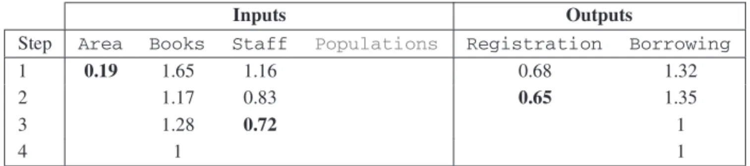
Table 10–Steps of ADEA stepwise algorithm for Tokyo libraries withoutPopulations.
Inputs Outputs
Step Area Books Staff Populations Registration Borrowing
1 0.19 1.65 1.16 0.68 1.32
2 1.17 0.83 0.65 1.35
3 1.28 0.72 1
4 1 1
Table 11–Steps of ADEA stepwise algorithm for Tokyo libraries withoutRegistration.
Inputs Outputs
Step Area Books Staff Populations Registration Borrowing
1 0.37 1.53 0.92 1.17 1
2 1.2 0.90 0.90 1
3 1.24 0.76 1
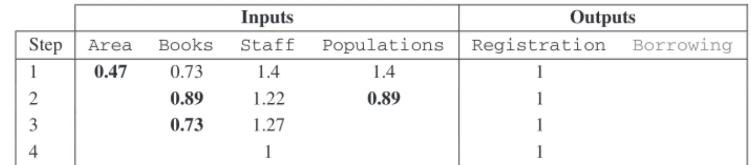
Table 12–Steps of ADEA stepwise algorithm for Tokyo libraries withoutBorrowing.
Inputs Outputs
Step Area Books Staff Populations Registration Borrowing
1 0.47 0.73 1.4 1.4 1
2 0.89 1.22 0.89 1
3 0.73 1.27 1
4 1 1
4 SELECTING A CRITICAL VALUE FOR LOADS. APPLICATION TO THE
ANALYSIS OF RESEARCH EFFICIENCY IN SPANISH UNIVERSITIES
The proposed methodology works dropping variables until some previously given value is reached by the loads. But until now, nothing is said about how such value can be selected. In this section an ad hoc Monte Carlo simulation is made in order to give a suitable value of such parameter. To do this, we will apply a DEA to obtain the research efficiency of the Spanish public universities in 2013. The data set, which has been calledSpanish University data set, has been obtained from official sources and includes one input
RP : The average number, considering the courses 2103, 2014 and 2015, of permanent research
professors from [22].
And seven outputs that measure the research production:
JCR : Number of articles published in journals indexed in the JCR. Number of published articles
indexed in “Main Collection of Web of Science (WoS)” in 2013 from [55].
RAR : Each permanent professor in Spanish universities can submit every six years his research
activity to be evaluate by the a national agency. This is the ratio between the number of positive evaluations and all the six years periods that they could submit to evaluation. Data comes from, CNEAI 2009 report [4], the report of the National Commission for the Evaluation of Research Activity.
RDP : Number of projects awarded in State Research and Development Programs, by the
Min-istry of Economy and Competitiveness in 2013) from [29, 30].
Phd : Number of doctoral thesis from database of doctoral thesis TESEO (Ministry of
Educa-tion, Culture and Sport) between 2007 and 2011 from [53].
STSR : Number of fellowships awarded for researcher training, Ministry of Education, Culture
and Sport in 2013 from [25, 26].
DE : Number of Doctorate programs with Mention towards Excellence, Ministry of Education
Culture and Sport in 2011 from [19, 20].
P : Number of patents registered between 2009 and 2013, Database of the Spanish Patent and
An output orientation is used to handle this model. The data have been obtained from the same official sources as the Granada ranking for 2013.
About output variableRARwe must say that it is a ratio and that there are many published works, as example [28, 21] disregarding the use of ratios in DEA. Also it must be said that there are many other works that use variables of type ratio as in [5, 37, 24]. In this case, the use of this variable is due to an attempt to reproduce as accurately as possible the original study with which to compare the results of the analysis.
4.1 Monte Carlo Simulation of Loads
Generally speaking, if we add a dummy, randomly generated, variable to a model and compute the load. Such load shows how much higher can be the load of a variable without meaning in the model, and a suitable quantile can be taken as lower limit for the load of the variables remaining in the model. But which distribution we can select to such dummy variable?
As a first try, we can consider the normal distribution. If we make a Shapiro-Wilk normality test to the variables in the initial Spanish universities model gets p-values from 10−7till 10−4except for one variable. A logarithmic transformation seems needed. After making that transformation all the new p-values of Shapiro-Wilk test are higher than 0.18. So a log-normal distribution is a good selection for the distribution of the dummy variable.
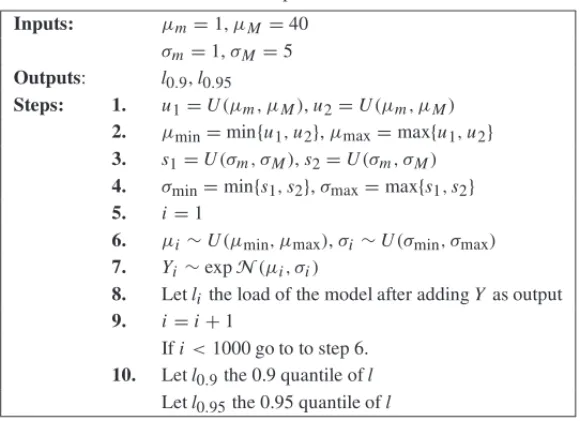
Table 13–n-th step of load simulation.
Inputs: µm=1,µM =40
σm=1,σM =5 Outputs: l0.9,l0.95
Steps: 1. u1=U(µm, µM),u2=U(µm, µM) 2. µmin=min{u1,u2},µmax=max{u1,u2} 3. s1=U(σm, σM),s2=U(σm, σM) 4. σmin=min{s1,s2},σmax=max{s1,s2} 5. i=1
6. µi ∼U(µmin, µmax),σi ∼U(σmin, σmax) 7. Yi∼expN(µi, σi)
8. Letli the load of the model after addingY as output 9. i=i+1
Ifi<1000 go to to step 6.
10. Letl0.9the 0.9 quantile ofl
Letl0.95the 0.95 quantile ofl
Table 13 shows how in each simulation two uniformly generated random values are taken from interval [1,40]. Let µmin the lower and µmax the higher. Ini-th step, from each of the one
thousand, an uniformly random generated valueµi are taken from[µmin, µmax]. Analogously,
And letσi an uniformly random generated value taken from[σmin, σmax]. The dummy variable
is generated asY ∼ exp(N(µi, σi)), added to the model and the load of it is calculated. The
0.9 and 0.95 quantiles of load are stored in a database. Taking into account that the loads are invariant by scale changes, the initial intervals chosen run through the values of the parameters that cross the sample values of the variables in the model.
Each simulation is repeated one thousand times, so 1 million of variables are generated and 1 million models are solved. The average value of 0.9 and 0.95 quantiles are 0.52 and 0.53. According to these, we must drop all variables in the model with load lower than 0.53. Table 14 shows that in first step the load ofJCRandSTSRare under 0.53.
Table 14–Stepwise ADEA for Spanish Universities data set.
Outputs
Step Model JCR RAR RDP Phd STRS DE P 1 IM 0.36 1.16 0.55 1.62 0.36 1.26 1.69 2 M1 0.35 1.04 0.60 1.52 1.10 1.39
3 M2 0.87 0.71 1.42 0.91 1.08
But if theSTFRvariable is removed from the model, a new simulation must be ran. The criterion for undoing draws is the same as previously applied. The new value for 0.9 and 0.95 quantiles are 0.55 and 0.57. And again the load ofJCRin step 2 is under this values.
A new simulation was made droppingSTSR and JCRvariables. And now the 0.9 and 0.95 quantiles are 0.54 and 0.62. But in this case the load of model in step 3, 0.71, is higher than 0.62, so no new simulation is needed.
Summarizing, 0.62 is an upper bound in 95% of cases when introducing a dummy variable in the model, thus 0.62 can be considered, with 95% of confidence, as a minimum value of the load of the variables in the model. Taking into account that the values obtained in the three simulations are around 0.6 and taking into account the meaning of the loads, we recommend this value as a general value for its use in the application of this methodology.
4.2 Variable selection
The application of the step-by-step algorithm, shown in Table 14, gives three models: the initial model that we will call IM, the resulting model of eliminating theSTSRvariable that we will call M1, and the resulting final model of eliminating the variablesSTSRandJCRthat we will call M2.
regis-Table 15–Efficiencies for some models DEA’s Spanish University.
University IM M1 M2 University IM M1 M2 A Coru˜na 2.46 2.46 2.46 Le ´on 2.13 2.13 2.13 Alcal´a 2.20 2.20 2.20 Lleida 1.59 1.59 1.59 Alicante 1.50 1.50 1.50 M´alaga 1.58 1.71 1.71 Almer´ıa 2.55 2.55 2.55 Mig. Hern´an. 1.11 1.11 1.13 Aut. Barcelona 1.12 1.12 1.12 Murcia 2.40 2.40 2.40 Aut. Madrid 1.36 1.36 1.36 Oviedo 3.05 3.05 3.05 Barcelona 1.32 1.32 1.42 Pab. Olavide 1.00 1.00 1.00 Burgos 1.23 1.23 1.23 Pa´ıs Vasco 1.57 1.57 1.57 C´adiz 1.38 1.38 1.38 Pol. Cartag. 1.28 1.28 1.28 Cantabria 1.51 1.51 1.53 Pol. Catalun. 1.00 1.00 1.00 Carlos III 1.32 1.32 1.32 Pol. Madrid 1.77 1.77 1.77 Cast. Mancha 2.20 2.20 2.20 Pol. Valencia 1.49 1.58 1.58 Comp. Madrid 2.14 2.14 2.14 Pomp. Fabra 1.00 1.00 1.00 C´ordoba 1.92 1.96 1.96 P´ub. Navarra 1.68 1.68 1.68 Extremadura 2.70 2.70 2.70 Rey J. Carlos 2.43 2.43 2.43 Girona 1.73 1.73 1.73 Rov. Virgili 1.00 1.00 1.00 Granada 1.60 1.79 1.79 Salamanca 1.82 1.82 1.82 Huelva 1.25 1.25 1.25 Santiago 1.45 1.58 1.58 Illes Balears 1.43 1.43 1.43 Sevilla 1.61 1.69 1.69 Ja´en 2.09 2.09 2.22 UNED 1.91 1.91 1.91 Jaume I 1.55 1.55 1.55 Valencia 2.63 2.66 2.66 La Laguna 3.47 3.47 3.47 Valladolid 2.36 2.54 2.54 La Rioja 1.14 1.14 1.14 Vigo 1.54 1.54 1.54 Las Palmas 3.85 3.85 3.85 Zaragoza 1.96 1.96 1.96
tered in RAR, since to obtain a six-years five articles are needed in JCR journals; for its part, the number of fellowships awarded for researcher training, collected inSTSR, depends heavily on the number of research projects, registered inRDP. We can conclude, then, that the final model hardly changes the efficiencies of the model that contains all the variables, but it is simpler and contains less redundant information.
In order to validate that the eliminated variables are indeed non-significant, the efficiencies as-sociated with each of the three models have been collected in Table 15. As can be seen in it the differences are very small and the Pearson correlation coefficient between the complete model and the other two models arerI M,M1 = 0.9993 yrI M,M2 = 0.9969, while the Spearman
co-efficients, which quantify the changes in the order, arerI M,M1 = 0.9983 yrI M,M2 =0.9918.
5 CONCLUSIONS AND FUTURE RESEARCH
We propose in this paper a new methodology for selecting variables in DEA models based on a measure of the contribution of the variables to the efficiency scores of the DMUs. A Monte Carlo simulation has been used to determine a suitable value for the minimum value that the load of the variables in the model must have. In this way a useful tool for decision makers is provided to test the role of a variable in a DEA model.
A cross-validation of the results obtained with the proposed methodology was carried out through the correlation coefficients between the different models obtained.
We have illustrated our procedure through one classical example in DEA: the Tokyo libraries data set, and using a new data set related to Spanish universities. In both cases, step by step results are provided.
At http://knuth.uca.es/shiny/DEA/an online interactive application is available. Some data example are ready to load to play with the software. Also, the user can upload its own data set and apply the algorithms proposed in this paper. It is our purpose to prepare a package for R for publication in R public repositories as free software.
As we have discussed above, we will try to compare technologies based on productivity rankings with DEA model, to compare Spanish public universities according to its research results.
The validation of the algorithms proposed through an extensive simulation and its development for other DEA models are some of the future lines of work.
REFERENCES
[1] ARAGAO DE˜ CASTROSENRALF, CESARNANCIL, SOARES DEMELLOJCCB & ANGULOMEZA L. 2007. Estudo sobre m´etodos de selec¸˜ao de vari´aveis em DEA.Pesquisa Operacional,27: 191–207.
[2] ADLERN & GOLANYB. 2001. Evaluation of deregulated airline networks using data envelopment analysis combined with principal component analysis with an application to Western Europe. Euro-pean Journal of Operational Research,132(2): 260–273.
[3] ADLERN & GOLANYB. 2002. Including principal component weights to improve discrimination in data envelopment analysis.Journal of the Operational Research Society,53(9): 985–991.
[4] AGRA¨IT N & POVES A. 2009. Informe sobre los resultados de las evaluaciones de la CNEAI. La situaci´on en 2009. http://www.mecd.gob.es/dctm/ministerio/ horizontales/ministerio/organismos/cneai/2009-info-v5.pdf?
documentId=0901e72b8008d9ff, June.
[5] AMINGR & TOLOOM. 2007. Finding the most efficient DMUs in DEA: An improved integrated model.Computers & Industrial Engineering,52: 71–77.
[6] ADLERN & YAZHEMSKYE. 2010. Improving discrimination in data envelopment analysis: PCA-DEA or variable reduction.European Journal of Operational Research,202: 273–284.
[8] BUELA-CASALG, BERMUDEZ´ MP, SIERRA JC, QUEVEDO-BLASCOR & CASTROA. 2010. Ranking de 2009 en investigaci´on de las universidades p´ublicas espa ˜nolas.Psicothema,22(2): 171– 179.
[9] BUELA-CASALG, BERMUDEZ´ MP, SIERRAJC, QUEVEDO-BLASCOR, CASTROA & GUILL´ EN-RIQUELMEA. 2011. Ranking de 2010 en producci´on y productividad en investigaci´on de las univer-sidades p´ublicas espa ˜nolas.Psicothema,23(4): 527–536.
[10] BUELA-CASALG, BERMUDEZ´ MP, SIERRAJC, QUEVEDO-BLASCOR, CASTROA & GUILL´ EN-RIQUELMEA. 2012. Ranking de 2011 en producci´on y productividad en investigaci´on de las univer-sidades p´ublicas espa ˜nolas.Psicothema,24(4): 505–515.
[11] BUELA-CASALG, BERMUDEZ´ MP, SIERRAJC, QUEVEDO-BLASCOR & GUILLEN-RIQUELME´ A. 2014. Ranking 2012 de investigaci´on de las universidades p´ublicas espa ˜nolas.Psicothema,26(2): 149–158.
[12] BUELA-CASALG, QUEVEDO-BLASCO R & GUILL´EN-RIQUELMEA. 2015. Ranking 2013 de investigaci´on de las universidades p´ublicas espa ˜nolas.Psicothema,27(4): 317–326.
[13] BIANY. 2012. A Gram–Schmidt process based approach for improving DEA discrimination in the presence of large dimensionality of data set.Expert Systems with Applications,39(3): 3793–3799.
[14] CHARNESA, COOPERWW & RHODESE. 1978. Measuring the efficiency of decision making units.
European Journal of Operational Research,2(6): 429–444.
[15] CHENY, MORITAH & ZHUJ. 2005. Context-Dependent DEA with an application to Tokyo public libraries.International Journal of Information Technology & Decision Making (IJITDM), 04(03): 385–394.
[16] COOPERWW, SEIFORDLM & TONEK. 2000.Data Envelopment Analysis: A Comprehensive Text with Models, Applications, References, and DEA-Solver Software. Kluwer Academic.
[17] COOKWD & ZHUJ. 2014. DEA Cobb-Douglas frontier and cross-efficiency.JORS,65(2): 265–268.
[18] DYSONRG, ALLEN R, CAMANHOAS, PODINOVSKIVV, SARRICO CS & SHALEEA. 2001. Pitfalls and protocols in DEA.European Journal of Operational Research,132: 245–259.
[19] BOLET´INOFICIAL DELESTADO, 20DEOCTUBRE DE2011.https://boe.es/boe/dias/
2011/10/20/pdfs/BOE-A-2011-16518.pdf.
[20] BOLET´IN OFICIAL DEL ESTADO, 30 DE JUNIO DE 2012. https://boe.es/boe/dias/
2012/06/30/pdfs/BOE-A-2012-8772.pdf.
[21] EMROUZNEJADA & AMINGR. 2009. DEA models for ratio data: Convexity consideration.Applied Mathematical Modelling,33(1): 486–498.
[22] ESTAD´ISTICA DE PERSONAL DE LAS UNIVERSIDADES. http://www. mecd.gob.es/educacion-mecd/areas-educacion/universidades/
estadisticas-informes/estadisticas/personal-universitario.html.
[23] FANCHONP. 2003. Variable selection for dynamic measures of efficiency in the computer industry.
International Advances in Economic Research,9(3): 175–188.
[25] BOLET´INOFICIAL DELESTADO, 4DESEPTIEMBRE DE2014.https://boe.es/boe/dias/ 2014/09/04/pdfs/BOE-A-2014-9081.pdf.
[26] BOLET´INOFICIAL DELESTADO, 8DEDICIEMBRE DE2014.https://boe.es/boe/dias/ 2014/12/08/pdfs/BOE-A-2014-12791.pdf.
[27] GONZALEZ-ARAYA´ MC & VALDES´ VALENZUELANG. 2009. M´etodos de seleccion de variables para mejorar la discriminacion en el analisis de eficiencia aplicando modelos DEA.Ingenieria Indus-trial,8(2): 45–56.
[28] HOLLINGSWORTH B & SMITH P. 2003. Use of ratios in data envelopment analysis. Applied Economics Letters,10(11): 733–735.
[29] PROYECTOS I+D EXCELENCIA CONCEDIDOS CONVOCATORIA. 2013. https://sede. micinn.gob.es/stfls/eSede/Ficheros/2014/Anexo_I_Ayudas_Concedidas_
Proyectos_ID_Excelencia_2013.pdf.
[30] PROYECTOSI+D+IORIENTADOS A LOS RETOS DE LA SOCIEDAD CONCEDIDOS EN LA CON-VOCATORIA. 2013.https://sede.micinn.gob.es/stfls/eSede/Ficheros/2014/ Anexo_I_Ayudas_Concedidas_Proyectos_I_D_I_Retos_2013.pdf.
[31] JENKINSL & ANDERSONM. 2003. A multivariate statistical approach to reducing the number of variables in data envelopment analysis.European Journal of Operational Research,147: 51–61.
[32] JITTHAVECHJ. 2016. Variable elimination in nested DEA models: a statistical approach.Int. J. Operational Research,27(3): 389–410.
[33] KAOL-J, LUC-J & CHIUC-C. 2011. Efficiency measurement using independent component anal-ysis and data envelopment analanal-ysis.European Journal of Operational Research,210(2): 310–317.
[34] LINTY & CHIUSH. 2013. Using independent component analysis and network DEA to improve bank performance evaluation.Economic Modelling,32: 608–616.
[35] LINSMPE & MOREIRAMCB. 1999. M´etodo I-O Stepwise para Selec¸˜ao de Vari´aveis em Modelos de An´alise Envolt´oria de Dados.Pesquisa Operacional,19(1): 39–50.
[36] LEWIN AY, MOREY RC & COOK TJ. 1982. Evaluating the administrative efficiency of courts.
Omega,10(4): 401–411.
[37] MORITAH & AVKIRANNK. 2009. Selecting inputs and outputs in data envelopment analysis by designing statistical experiments.Journal of the Operations Research Society of Japan,52(2): 163– 173.
[38] MADHANAGOPALR & CHANDRASEKARANR. 2014. Selecting Appropriate Variables for DEA Using Genetic Algorithm (GA) Search Procedure.International Journal of Data Envelopment Anal-ysis and Operations Research,1(2): 28–33.
[39] NATARAJANR & JOHNSONAL. 2011. Guidelines for using variable selection techniques in data envelopment analysis.European Journal of Operational Research,215: 662–669.
[40] NORMAN M & STOKERB. 1991.Data Envelopment Analysis: The Assessment of Performance. Wiley.
[41] BASE DE DATOS DE LA OFICINA ESPANOLA˜ DE PATENTES Y MARCAS. http: //www.oepm.es/es/sobre_oepm/actividades_estadisticas/estadisticas/
[42] PASTORJT, RUIZJL & SIRVENTI. 2002. A statistical test for nested radial DEA models.Operations Research,50(4): 728–735.
[43] R CORETEAM. 2014. R: A Language and Environment for Statistical Computing.
[44] RUGGIEROJ. 2005. Impact assesment of input omission on DEA.International Journal of Informa-tion Tchnology and Decission Making,46(3): 359–368.
[45] SIGALAM, AIREY D, JONES P & LOCKWOODA. 2004. ICT Paradox Lost? A stepwise DEA methodology to evaluate technology investments in tourism settings.Journal of Travel Research,43: 180–192, November.
[46] SOARES DEMELLOJCCB, GONC¸ALVESGOMESE, ANGULOMEZAL & ESTELLITALINSME. 2004. Selecci´on de variables para el incremento del poder de discriminaci´on de los modelos DEA.
Investigaci´on Operativa,XII(24), May.
[47] SMITHP. 1997. Model misspecification in Data Envelopment Analysis.Annals of Operations Re-search,73(0): 233–252.
[48] SIRVENTI, RUIZJL, BORRAS´ F & PASTORJT. 2005. A Monte Carlo Evaluation of several Tests for the Selection of Variables in Dea Models.International Journal of Information Technology and Decision Making,4(3): 325–344.
[49] SEXTONTR, SILKMANRH & HOGANAJ. 1986. Data Envelopment Analysis: Critique and exten-sions.New Directions for Program Evaluation,1986(32): 73–105.
[50] SUBRAMANYAMT. 2016. Selection of Input-Output Variables in Data Envelopment Analysis-Indian Commercial Banks.International Journal of Computer & Mathematical Sciencies,5(6): 51–57, June.
[51] SIMARL & WILSONPW. 2001. Testing restrictions in nonparametric efficiency models. Communi-cations in Statistics – Simulation and Computation,30(1): 159–184.
[52] SHARMAMJ & YUSJ. 2015. Stepwise regression Data Envelopment Analysis for variable reduction.
Applied Mathematics and Computation,253(0): 126–134.
[53] BASE DE DATOS DE TESIS DOCTORALES.https://www.educacion.gob.es/teseo.
[54] UEDAT & HOSHIAIY. 1997. Application of principal component analysis for parsimonious summa-rization of DEA inputs and/or outputs.Journal of the Operations Research Society of Japan,40(4): 466–478.
[55] BASES DE DATOS DE LA WEB OF SCIENCE. https://www.recursoscientificos. fecyt.es.