CENTRO DE CI ˆENCIAS EXATAS E DE TECNOLOGIA
PROGRAMA DE P ´OS-GRADUAC¸ ˜AO EM CI ˆENCIA DA COMPUTAC¸ ˜AO
BRAIN COMPUTER INTERFACE FOR
DETECTING DROWSINESS USING
INSTANCE-BASED LEARNING APPROACH
A
MIRJ
ALILIFARDO
RIENTADOR: P
ROF. D
R. E
DNALDOB
RIGANTEP
IZZOLATOS˜ao Carlos – SP
CENTRO DE CI ˆENCIAS EXATAS E DE TECNOLOGIA
PROGRAMA DE P ´OS-GRADUAC¸ ˜AO EM CI ˆENCIA DA COMPUTAC¸ ˜AO
BRAIN COMPUTER INTERFACE FOR
DETECTING DROWSINESS USING
INSTANCE-BASED LEARNING APPROACH
A
MIRJ
ALILIFARDQualificac¸˜ao apresentada ao Programa de P´os-Graduac¸˜ao em Ciˆencia da Computac¸˜ao da Univer-sidade Federal de S˜ao Carlos, como parte dos requi-sitos para a obtenc¸˜ao do t´ıtulo de Mestre em Ciˆencia da Computac¸˜ao, ´area de concentrac¸˜ao: Computation Methodologies and Techniques
Orientador: Prof. Dr. Ednaldo Brigante Pizzolato
S˜ao Carlos – SP
Uma interface cérebro-computador (ICC, BCI em inglês), também chamada interface mente-máquina (IMM), e também interface neural direta (IND), interface telepática sintética (ITS) ou interface cérebro-máquina, é um caminho comunicativo direto entre o cérebro e um dispositivo externo. Essa cria a possibilidade de usuário controlar um sistema ou um ambiente sem necessidade de usar os músculos. Além disso, a ICC possibilita a gravar e analisar as atividades neuropsicológicas de um indivíduo. Claramente a aplicação da ICC aumentou significativamente durante a década passada. Entre várias
aplicações dele, recentemente, pesquisadores tem se interessado em uso dos sinais EEGs na área de segurança ao volante. A condução sonolenta é uma das maiores causas de acidentes nas rodovias do país. Essa pesquisa tem como objetivo o desenvolvimento de um sistema de detecção de sonolência por meio de uma abordagem eficiente baseada em algoritmo K-nearest neighbors (K-NN). Na primeira fase a distribuição de energia dos sinais EEG foi obtida usando uma transformação de Fourier (STFT) e depois o valor médio de energia em períodos de tempo de 0.5 segundos, desvio padrão e entropia Shanon foram calculados para cada das sub-frequências de EEG. Por fim, 52 características foram extraídas. O
algoritmo Random Forest foi aplicado nesses dados afim de os atributos mais informativos entre os demais. Finalmente 11 características foram selecionados foram selecionados para classificar a
Brain Computer Interface (BCI) is a way to establish a communication between brain and computers. It allows the users to control a computer system and even an environment without moving a muscle or it allows the computer to record and analyze the user’s neu-ropsychological brain activities. Clearly, the range of BCI applications has increased in the past decade due to the use of modern machine learning and signal processing methods. Among various applications of BCI, lately the use of EEG records for driver safety has been considered by some researchers. Drowsy driving is a major cause of many traffic accidents. The aim of this work is to develop an automatic drowsiness detection system using an efficient k-nearest neighbors (K-NN) algorithm. First, the distribution of power in time-frequency space was obtained using short-time Fourier transform (STFT) and then, the mean value of power during time-segments of 0.5 second was calculated for each EEG sub-band. In addition, standard deviation (SD) and Shanon entropy related to each time-segment were computed from time-domain. Finally, 52 features were extracted. Random forest algorithm was applied over the extracted data, aiming to choose the most informative subset of features. A total of 11 features were selected in order to classify drowsiness and alertness. The Kd-tree algorithm was used as the nearest neighbors search algorithm so as to have a fast classifier. Our experimental results show that drowsiness can be classified efficiently with 91% accuracy using the methods and materials proposed in this paper. We also compared the classification results obtained by K-NN (as an instance-based learning algorithm) with four well-known classifiers including decision tree, support vector machine, logistic regression and naive bayes.
2.1 Cognitive electrophysiology is a field defined by a spectrum from cognitive to
electrophysiology. As soon as a researcher Knows where the working area is on
this spectrum, this will guide his experiments, hypotheses, data analysis, target
journals and conferences. (COHEN, 2014) . . . 21
2.2 A diagrammatic representation of 10-20 electrodes settings for 75 electrodes
including the reference electrodes: (a) and (b) represent the tree-dimensional
measures, and (c) indicates a two-dimensional view of the electrode setup
con-figuration(COHEN, 2014) . . . 22
2.3 A) The grand-averaged ERP waveforms for Loss 50 and Gain 50 conditions;
B) Theta bands during Loss 50 at FZ electrode and Gain 50 at CZ electrode are
shown. Alcoholics showed decreased amplitude in theta (37 Hz) band more
an-teriorly (frontal) for the loss condition and more posan-teriorly (centro-parietal) for
the gain condition. C) Topographic maps of theta (3-7 Hz) power in control and
alcoholic groups illustrating that the loss condition had an anterior topography
and the gain condition had a posterior topography. Decreased theta band power
in alcoholics in both conditions is illustrated; D) Time-frequency (TF) plots
du-ring the loss condition at the Fz electrode in the alcoholic and control groups;
and E) TF plots during the gain condition at the Cz electrode. The square box
inside TF plots marks the time-frequency region of interest, namely the time
interval of 200-500 ms across the theta frequency range 3-7 Hz for analysis.
A) EEG in different frequency bands at one location in the contralateral hand
area of motor cortex from one subject differentiates left and right movement
directions. B) Color-coded shading of average data from five subjects
illustra-tes the information about hand movement direction provided by EEG recorded
over different cortical areas. C) Colored-coded shading of average data from six
subjects illustrates the information over production of different vowels provided
by EEG recorded over different cortical areas. (LEUTHARDT et al., 2004) . . 25
2.5 The tree dimensions that show frequency, power and phase (COHEN, 2014) . . 26
2.6 Raw EEG data showing oscillation at different speeds and for different lengths
of time. Each line corresponds to a specific electrode (SAŁABUN, 2014) . . . 26
2.7 The data cube containing information over time, frequency and space. Since it
is difficult to view a 3-D cube, it is sliced in four points of view. (COHEN, 2014) 28
3.1 SVM finds the widest hyperplane. Support vectors are shown with a red border
(XU et al., 2009) . . . 34
3.2 Relationship of a dichotomous outcome variable with a continuous predictor
(PENG; LEE; INGERSOLL, 2002) . . . 37
3.3 K-nearest neighbors search using kd-trees . . . 42
4.1 EEG signals showed in two points (A and B) before and after noise eliminations.
The red signals are noisy and the blue traces indicate the EEG after processing
using an artifact removal algorithm (ZEMAN, 2012) . . . 54
5.1 The block diagram of the our method . . . 64
5.2 The mean energy of EEG sub-bands related to drowsiness and wakefulness of
11 subjects. A higher mean energy of Frequency=1 Hz is observable. . . 65
5.3 The mean energy of EEG sub-bands related to drowsiness and wakefulness of
11 subjects. A higher mean energy of Frequency=6 Hz is observable. . . 65
5.4 The mean energy of EEG sub-bands related to drowsiness and wakefulness of
11 subjects. A higher mean energy of Frequency=49 Hz is observable. . . 66
5.5 The mean energy of EEG sub-bands related to drowsiness and wakefulness of
11 subjects. A higher mean energy of Frequency=50 Hz is observable. . . 66
6.1 The classification performance of feature dimension for correctly classified
ins-tances. . . 71
6.2 The classification accuracy of mean energy, mean energy and Standard
Devia-tion, and mean energy, Standard Deviation and Entropy together. . . 72
6.3 The votes of 10 classifications during 5 seconds are gathered and the majority
vote is considered as the conciousness state during each specific time period. . . 75
6.4 K-NN classification time using linear and kd-trees search . . . 76
6.5 An accuracy comparison between five different classifiers using the data
obtai-ned through the proposed approach. . . 79
6.6 An accuracy comparison between subject-dependent and subject-independent
4.1 Karolinska sleepiness scale (KSS). . . 47
4.2 List of previous works on driver drowsiness detection using behavioral measures. 50
4.3 List of previous works on driver drowsiness detection using behavioral measures. 51
4.4 Advantages and limitations of various measures. . . 55
4.5 List of previous works on driver drowsiness detection using biosignal measures. 56
4.6 List of previous works on driver drowsiness detection using machine learning
approach and just EEG signal. . . 58
4.7 List of previous works on driver drowsiness detection using machine learning
approach and just EEG signal. . . 59
5.1 The ordered list of 11 most important features. Each feature is related to time
segments of 0.5 second . . . 69
6.1 The classification accuracy of drowsiness based on the number of features
en-gaged in classification task. . . 71
6.2 The classification accuracy and time for different values of feature dimensions,
using linear search. Letterdrepresents the feature dimension . . . 73
6.3 The classification accuracy and time for different values of feature dimensions,
using kd-trees search algorithm. Letterdrepresents the feature dimension . . . 73
6.4 The accuracy and classification time after using Random Forest and PCA . . . 74
6.5 Classification accuracy, precision and sensitivity for both drowsiness and
wake-fulness stages . . . 75
6.6 An efficiency comparison of the current approach and the preliminary proposals
known classification algorithms . . . 79
6.8 The subject-dependent classification accuracy for 11 subjects for K-NN where
ANN–Artificial Neural Network
BCI–Brain Computer Interface
BMI–Brain Machine Interface
BTLE–Bluetooth Low Energy
CCD–Charge-Coupled Device
DFS–Discrete Fourier Series
DFT–Discrete Fourier Transform
DTFT–Discrete-Time Fourier Transform
DVR–German Road Safety Council
DWT–Discrete Wavelet Transform
ECG–Electrocardiography
ECoG–Electrocorticography
EEG–Eletroencefalograma
EMG–Electromyogram
ERP–Event Related Potential
EoG–Electrooculogram
FFT–Fast Fourier Transform
FT–Fourier Transform
HF–High Frequency
KNN–K-Nearest Neighbors
KSS–Karolinska Sleepiness Scale
LDA–Linear Discriminant Analysis
LF–Low Frequency
LIBLI–A Library for Large Linear Classification
MAC–Medium Access Protocol
MANET–Mobile Ad hoc Network
MEG–MagnetoEncephaloGraphy
MI–Motor Imagery
MVC–Motor Vehicle Collision
NHTSA–National Highway Traffic Safety Administration
NREM–Non-Rapid Eye Movement
NSF–National Sleep Foundation
PERCLOS–Percentage of Eyelid Closure
PET–Positron Emission Tomography
REM–Rapid Eye Movement
SDK–Software Development Kit
SDLP–Standard Level for Normal Drivers
STFT–Short-Time Fourier Transform
SVM–Support Vector Machine
SWM–Steering Wheel Movement
SWS–Slow Wave Sleep
VLP–Variation of Lane Position
WKNN–Weighted K-Nearest Neighbors
GLOSS ´ARIO
CHAPTER 1 – INTRODUCTION 14
1.1 Summary . . . 19
CHAPTER 2 – THEORETICAL BASIS 20 2.1 What is Cognitive Electrophysiology? . . . 20
2.2 Diving into EEG . . . 21
2.2.1 Event Related Potential . . . 23
2.2.2 Image Motory . . . 24
2.2.3 EEG Processing Techniques . . . 25
2.2.4 Time-Domain . . . 26
2.2.5 Frequency-Domain and Fourier Transform . . . 27
2.2.6 Ways to view Time-Frequency Results . . . 27
2.2.7 Brain Frequency Bands . . . 28
2.3 Sleep EEG . . . 29
2.3.1 Sleep Stages . . . 29
2.4 EEG Equipments and Research Costs . . . 30
2.5 Summary . . . 31
CHAPTER 3 – CLASSIFICATION AND FEATURE SELECTION 33
3.2 Naive Bayes . . . 35
3.3 Decision tree . . . 36
3.4 Logistic regression . . . 37
3.5 Instance-based learning . . . 38
3.5.1 Flexible inductive bias . . . 38
3.5.2 Learning parameters does not need to be fixed in advance . . . 38
3.5.3 Instance-based can cover the global local spectrum . . . 39
3.5.4 K-nearest neighbors (K-NN) . . . 39
3.6 Kd-Tree . . . 41
3.7 Feature selection for demensionality reduction . . . 42
3.7.1 Principal component analysis (PCA) for feature selection . . . 42
3.7.2 Random forest algorithm for feature selection . . . 43
3.8 Summary . . . 44
CHAPTER 4 – LITERATURE REVIEW 45 4.1 Subject measures . . . 46
4.2 Vehicle-based measures . . . 48
4.2.1 Steering wheel movement (SWM) . . . 48
4.2.2 Standard Deviation of lane position (SDLP) . . . 49
4.3 Behavioral measures . . . 49
4.4 Biosignal measures . . . 53
4.5 Summary . . . 60
CHAPTER 5 – RESEARCH PROCESS 61 5.1 Goals . . . 61
5.2.2 Signal processing and feature extraction . . . 63
5.2.3 Feature selection and classification . . . 68
5.3 Summary . . . 69
CHAPTER 6 – EXPERIMENTAL RESULTS AND DISCUSSION 70 6.1 Experiment 1 - Measuring the performance of selected features for drowsiness detection . . . 70
6.1.1 Classification accuracy for distinct feature dimension . . . 70
6.1.2 The effectiveness of mean energy, Standard Deviation and entropy . . . 72
6.2 Experiment 2 - Classification results . . . 73
6.2.1 Classification performance with and without using demensionality re-duction and optimized nearest neighbors search . . . 73
6.2.2 Classification performance using the dataset provided by Random Fo-rest and PCA . . . 74
6.2.3 Alertness and drowsiness classification . . . 74
6.2.4 Drowsiness detection using the majority vote . . . 75
6.2.5 Effectiveness of proposed approach by means of accuracy and classifi-cation time . . . 76
6.3 Experiment 3 - Comparing results with others from the literature . . . 77
6.4 Experiment 4 - Comparing the classification results of K-NN with four other classification algorithms . . . 78
6.4.1 SVM . . . 79
6.4.2 Decision tree . . . 80
6.4.3 Logistic regression . . . 80
6.4.4 Naive Baye . . . 80
6.5 Experiment 5 - Classifying data of each subjects independently . . . 81
7.1 Contributions . . . 86
7.2 Publication . . . 86
7.3 Future works . . . 86
REFER ˆENCIAS 88
Chapter 1
I
NTRODUCTION
This chapter presents the general context and motivation of this research, and the goals that the current investigation aims to achieve.
Brain-computer interface (BCI) (or brain-machine interface (BMI) for some researchers)
es-tablishes a direct interface between the brain and some external device. The basic idea is to
capture the thoughts by inspecting the brain waves. There are basically two means to do so:
invasive and non-invasive. Invasive methods rely on objects (like electrodes or chips) or
subs-tances (like chemical molecules) introduced into the brain of a subject or animal. On the other
hand, non-invasive methods do not require object implantation or drug inoculation into subjects
(or animals) brain (or body). Usually, the subject interacts with the computer system through
wearable devices. The fundamental concept is that the brain signal bypasses the normal output
pathways of the body.
At the beginning, BCI researches focused on fundamental applications such as prompt
con-trol. Later on, the researches focused on applications for paralyzed patients or for cases with
locked-in syndrome. Nowadays, the area has experienced more alternative applications in
he-althy human subjects. One could point out the use of modern machine learning and signal
processing methods as the reason for the increase of BCI applications in the past decade. Some
of the main applications of this area are: communication, prosthetic control, robotics and
secu-rity.
One of the investigation areas that has always been considered by researchers is safety
related subjects where the main focus is on making the daily activities more secure, specially
in the environments that tend to involve in a greater than average number of accidents. Since
the human errors is one of the major causes of daily accidents, lately BCI researches have
human-made mistakes that may cause irreparable causalities.
A traffic collision, also known as motor vehicle collision (MVC), traffic accident or car
crash occurs when a vehicle collides with another vehicle, pedestrain, animal, road debris or
other stationary obstruction that may result in injury, death or property damage. A number
of non-human factors contribute to the risk of collision, including vehicle design, speed of
operation and road design. However, human-caused factors such as driver skill, impairment
due to alcohol or drugs, behavioral causes, the lack of concentration and drowsiness play a
significant role in road accidents (SAHAYADHAS; SUNDARAJ; MURUGAPPAN, 2012a).
Human factor in vehicle collision includes all factors related to human ability to control the
vehicle, such as visual and authority acuity, psychological behaviors, reaction speed and
deci-sion making ability. A report in 1985 relying on the British and American crush data showed
that the driver impairment contribute about 93% of vehicle crushes (LUM; REAGAN, 1995).
Driver impairment describes the factors that may prevent driving in a normal level of skills.
Common impairments include:
1. Alcohol: According to the government of Canada, coroner reports from 2008 reported
that almost 40% of fatally injured drivers had consumed some quantity of alcohol.
2. Physical Impairment: Including poor eyesight or other physical impairments that may
cause collision.
3. Drug use: Including some prescription drugs, over the counter drugs (notably
antihista-mines, opioids and muscarinic antagonists) and illegal drugs.
4. Distraction: Any external stimuli that can affect the driver’s attention, for example,
con-versation with passengers, operating the cellphone or distracting sounds are source of
distractions that can cause losing the normal driving state.
5. Drowsiness: Falling sleep suddenly as a result of sleep disorders(e.g. Narcolepsy) or
sleep deprivation can lead to losing the car control and putting the car passengers life at
risk.
6. Combination of factors: Several aforementioned causes can be combined and result in a
much worse situation.
The US National Highway Traffic Safety Administration (NHTSA), conservatively
estima-ted that a total of 100,000 vehicle crashes in each year are the direct result of driver drowsiness.
monetary losses (RAU, 2005). In 2009, the US National Sleep Foundation (NSF) reported that
54% of adult drivers have driven a vehicle while feeling drowsy, and 28% of them actually fell
asleep. The German Road Safety Council (DVR), claims that one in four highway traffic
fata-lities is due to the momentary driver drowsiness (HUSAR, 2012). These statistics suggest that
driver’s drowsiness is one of the main causes of road accidents.
A driver who falls asleep at the wheel, loses the control of the vehicle, an action which
often results in a crash with either another vehicle or stationary objects. In order to prevent
these devastating accidents, the state of drowsiness of the driver should be monitored. The
following measures have been widely used for monitoring drowsiness:
1. Vehicle-based measures: A number of metrics, including deviations from lane position,
movement of the steering wheel, pressure on the acceleration pedal, etc., are constantly
monitored and any change that crosses a specified threshold indicates a significantly
in-creased probability that the driver is drowsy (FORSMAN et al., 2013) , (LIU; HOSKING;
LENN ´E, 2009).
2. Behavioral measures: The behavior of the driver, including yawning, eye closure, eye
blinking, head pose, etc., is monitored through a camera and the driver is alerted if any of
these drowsiness symptoms are detected (FAN; YIN; SUN, 2009), (AKIN et al., 2008).
3. Biomeasures: The correlation between biological signals (electrocardiogram (ECG),
elec-tromyogram (EMG), electrooculogram (EoG) and electroencephalogram (EEG)) and
dri-ver drowsiness has been studied by many researchers (KOKONOZI et al., 2008), (KHUSHABA
et al., 2011), (YANG; LIN; BHATTACHARYA, 2010).
Other than these three, researchers have also used subjective measures, where drivers are
asked to rate their level of drowsiness either verbally or through a questionnaire. The intensity
of drowsiness is determined based on standard rating (KHUSHABA et al., 2011), (TREMAINE
et al., 2010).
Vehicles-based measures can function reliably only at particular environments and are too
dependent on the geometric characteristics of the road and to a lesser extent on the kinetic
characteristics of the vehicle (LEW et al., 2007). Furthermore, several studies showed that they
are poor predictors of performance error risk due to drowsiness (SIMONS et al., 2012), (DAS;
ZHOU; LEE, 2012) . Moreover, vehicular-based metrics are not specific to drowsiness. As an
example, standard deviation of lane position can also be caused by any type of impaired driving,
The drowsiness detection using behavioral measures have promissing results, although the
majority of researches are conducted in a controlled environments like simulations.
Unfortuna-tely, the positive detection rate is decreased significantly when the experiment was carried out
in a real environment (PHILIP et al., 2005a). Additionally, driver state cannot be correlated to
driving performance which is a major shortcoming of these measures.
Regarding the subjective measures, since the level of drowsiness is measured during long
periods of time (several minutes), sudden variations cannot be detected using this kind of
me-asures. Another limitation of using subjective ratings is that the self-introspection alerts the
driver, thereby reducing their drowsiness level (SAHAYADHAS; SUNDARAJ;
MURUGAP-PAN, 2012a).
The previously described measures become apparent only after the driver starts to sleep,
which is often too late to prevent an accident. Unlike the aformentioned measures, bio-signals
start to change in earlier stages of drowsiness. Hence, they are more adequate to detect
drowsi-ness by making it possible to alert a drowsy driver in a timely manner and thereby prevent many
road accidents. Various approaches have been selected to detect and prevent the accidents
cau-sed by drowsiness or distraction sources (KAPTEIN; THEEUWES; HORST, 1996) (KURT et
al., 2009), however emerging electroencephalogram (EEG) opened new research area in terms
of analyzing brain activity through different tasks, such as driving. Using EEG, it is possible to
investigate almost all the physical and behavioral activities. Accordingly, EEG processing can
be utilized to analyze individual’s central nervous system activity through a driving task and
evaluate the consciousness and attention level in order to predict and prevent the probable risky
situations.
Using EEG with several electrodes, has been proven that it is possible to detect and analyze
brain activity changes accurately, although the main lack of EEG equipments with many
elec-trodes is their intrusive nature. In order to make EEG equipments more applicable in day to
day life experiments, non-intrusive systems were introduced (YU, 2009) (BAEK et al., 2012).
The reliability and accuracy of driver drowsiness detection by using bio-signals is high
compa-red to other methods (SAHAYADHAS; SUNDARAJ; MURUGAPPAN, 2012b). However, the
intrusive nature of measuring bio-signals remains an issue to be addressed. This is specially
challenging because the less electrode, the less information related to brain neural activities is
obtained. Consequently, the detection accuracy may decrease significantly.
For preventing car accidents caused by sleepiness, the system should detect drowsiness
accuratly and rapidly. Thus, systems by which drowsiness is detected within long periods of
ideal system also is expected to be non-intrusive and uses less electrodes. These factors imply
that drowsiness ought to be detected based on few numbers of EEG samples, which means
finding the best possible EEG features that carry enough information about neurons activities
during somnolence.
For recognizing drowsiness stage, EEG data must be classified. Regarding the fact that
microcontroller device would be used in real experiments (because it is not realistic to use
a computer in a limited environment like car), preferably the classification algorithm ought
to be fast and easily implementable. Unlinke most learning algorithms, case-based, also
cal-led instance-based approaches do not construct an abstract hypothesis but instead base
clas-sification of test instances on similarity to specific training cases (AHA; KIBLER; ALBERT,
1991). Instance-based approach postpone generalization until a new instance must be
classi-fied. Another characteristic of this approach is that rather than estimating the target function
for the entire instance space, the target function is estimated locally and differently for each
new instance. In instance-based method, the training is typically simple and fast. Also, it has
the ability to learn complex target functions and not to lose information. However, the
perfor-mance is reduced in high dimensional case, due to the curse of dimensionality (AGGARWAL,
2014). While the aformentioned characteristics of instance-based method make it an
appro-priate candidate to be engaged in drowsiness detection task, at the same time, the decline in
performance in high demensional feature spaces makes it questionable whether it is possible to
reduce drowsiness EEG features to a number of features so that an instance-based method can
perform well.
Several studies have found evidences that neural oscillations and EEG sub-bands’ activities
have specific patterns during drowsiness and wakefulness (CANTERO et al., 1999),
(CAN-TERO; ATIENZA; SALAS, 2002). Foong et al. reported a higher Alpha and Theta band
power, specially in the frontal, central, parietal and occipital areas, during drowsiness (FOONG
et al., 2015). Based on these evidences, since the power of EEG sub-bands and other
charac-teristics of EEG activity of drowsiness differ from alertness then, each of these consciousness
stages occupies a specific area in feature space. Regarding the fact that k-nearest neighbors,
as an instance-based method, approach tends to partition the feature space into sub-spaces and
then classifies each point based on its nearest neighbors, therefore, we assume that when the
dimensionality isn’t high, K-NN along with kd-trees —as an efficient search algorithm for
pro-blems with moderate number of dimensions (SKIENA, 1998) —has the ability to classify EEG
1.1
Summary
In this capter, we introduced the state of problem and justified the general purpose of the
current work. The organization of this document is as follows: Section 2, expatiates neural
signal processing and EEG classification techniques. Section 3, reviews the related works in
BCI, and then those researches in which sleep detection using EEG techniques were considered
as the main idea. In section 4, we will talk about the classification algorithms and the way
they may classify the EEG dynamics. The proposed method for detecting and classifying low
consciousness level is discussed in Section 5. The last section is allocated to describe the
Chapter 2
T
HEORETICAL
B
ASIS
In this chapter, we will go through a number of techniques of EEG signal analysis that helps understanding how to analyse neural time-series data.
2.1
What is Cognitive Electrophysiology?
Cognitive electropsychology is the study of how cognitive functions including memory,
perception, language, social cognition, behavioral monitoring and emotions are generated by
electrical activity produced through the population of neurons.
Cognitive electropsychology is a field of a vast and fundamentally different scientific area
due to its multi-aspect essence. On one end, medical-oriented researches try to analyze cognitive
signals, understanding the physiological-related issues. For these scientists, electropsychology
is useful because it is much more precise than behavioral measures or self-reports. In these fields
of research, understanding neural mechanism is relevant, but ultimately the goal of research
is to dissect and understand the cognitive components of physical rather than psychological
properties of brain (COHEN, 2014).
On the other end, psychologists are passionate about reading the electropsychological data,
being able to find the relation between behavioral activities and brain’s neural activities. For
these group of researchers, analyzing the data provided by electropsychology can help them to
relate the external human behavior with brain neural interactions.
Engineers hold the other end of this conceptual triangle (HASSANIEN; AR, 2015). They
are interested in electropsychology in order to developing the Brain-Computer tools and
unders-tanding the neural patterns respected to psychological or physical activities. For these scientists,
using these precise data, they can link human nerobiological or neuropsychological process
to computational models. Here, analyzing the sophisticated data and interpretating
neropsy-chological signals are crucial. At this spectrum, electrical and computer engineers have their
own distinct way to analyze and extract the data they need, in order to develop their favorite
tools. Electrical engineers mostly tend to use signal processing techniques along with various
digital tools to extract the favorite features from signals. Unlike the previous group, computer
engineers incline to use basic signal processing techniques and then using machine learning
al-gorithms, with the purpose of relating extracted features from neural interactions to the external
psychological or biological phenomenons, and then using the results to develop Brain Computer
Interface (BCI) applications.
Every researcher who works in BCI related studies, may find himself somewhere between
two extremes(Figure 2.1) and it is useful for him to think where to place himself because it will
help knowing how much time should be devoted to reading cognitive psychology papers versus
neuroscience papers, and what kind of analysis should be performed on data.
Figure 2.1: Cognitive electrophysiology is a field defined by a spectrum from cognitive to elec-trophysiology. As soon as a researcher Knows where the working area is on this spectrum, this will guide his experiments, hypotheses, data analysis, target journals and conferences. (COHEN, 2014)
2.2
Diving into EEG
The brain activity provides several types of signals including magnetic, metabolic and
elec-trical. Magnetic fields can be recorded with MagnetoEncephaloGraphy (MEG); brain metabolic
activity related to blood flow can be captured with Positron Emission Tomography (PET) or
functional Magnetic Resonance Imaging (fMRI); electrical signals can be acquired through
Electro-Encephalography (EEG) (MAKEIG et al., 2012). EEG was first recorded by German
psychiatrist Hans Berger (BERGER, 1929) through the use of several electrodes attached to the
human skull. EEG is regarded to be the fastest and less expensive way to capture the brain
sig-nals and the advances in bio-sensor technologies for EEG have opened up brainwave research
and application development at an unprecedented level in recent years.
Technically speaking, the brain has several distinct areas and landmarks such as Nasion,
in order to capture the areas activities. If they are on the scalp, one can get the EEG
measu-res; if they are on the surface of the brain, it is possible to get the ECoG measures (from the
cortical surface with higher spatial resolution than EEG and less susceptible to ambient noise).
An international system called 10-20 (see 2.2) was created in order to provide a naming and
positioning scheme for EEG applications. Originally, the 10-20 system had only 19 electrodes
which were later increased to more than 70. This number can be raised up to 210 electrodes.
Figure 2.2: A diagrammatic representation of 10-20 electrodes settings for 75 electrodes including the reference electrodes: (a) and (b) represent the tree-dimensional measures, and (c) indicates a two-dimensional view of the electrode setup configuration(COHEN, 2014)
.
For each EEG recording, it is mandatory to choose a reference electrode which should
ideally, be affected by global voltage changes in the same manner as all the other electrodes.
This reference electrode allows canceling out brain unspecific activity (e.g. slow voltage shifts
bone behind the ears). It is also possible to compute the average reference when the system has
multi-channels.
2.2.1
Event Related Potential
An Event-Related Potential (ERP) is any stereotyped electrophysiological response to an
internal or external stimulus. In simple terms, it is any measured brain response that is the direct
result of a thought process or perception. This stimulus can be a specific sensory, cognitive or
motor event (LUCK, 2014). The Event Related Potential signals can be negative (e.g. N100,
N400) or positive (e.g. P300), and they are named based on the exact time in which they
appeared after an internal or external stimuli.
ERPs are measured by EEG signals and it has been found that an event related potential
across the parieto-central area of the skull is usually captured around 300ms after the target
stimulus, and it is called P300. In other words, P300 is a positive deflection in human event
related potential (PICTON, 1992). The P300 potential is characterized by a positive deflection
in the EEG amplitude at latency of approximately 300ms after the target stimulus is presented
within a random sequence of non-target stimuli. Elicitation time and amplitude are correlated
to user’s fatigue and to saliency of stimulus (color, contrast, brightness, etc.).
This potential is always presented as long as the user is attending to the process, and its
variability among users is relatively low. Also the amplitude of ERP can be different for distinct
subjects based on their psychological or physical state. For instance, P300 shows different
Figure 2.3: A) The grand-averaged ERP waveforms for Loss 50 and Gain 50 conditions; B) Theta bands during Loss 50 at FZ electrode and Gain 50 at CZ electrode are shown. Alcoholics showed decreased amplitude in theta (37 Hz) band more anteriorly (frontal) for the loss condition and more posteriorly (centro-parietal) for the gain condition. C) Topographic maps of theta (3-7 Hz) power in control and alcoholic groups illustrating that the loss condition had an anterior topography and the gain condition had a posterior topography. Decreased theta band power in alcoholics in both conditions is illustrated; D) Time-frequency (TF) plots during the loss condition at the Fz electrode in the alcoholic and control groups; and E) TF plots during the gain condition at the Cz electrode. The square box inside TF plots marks the time-frequency region of interest, namely the time interval of 200-500 ms across the theta frequency range 3-7 Hz for analysis. (CHELLA, 2012)
ERPs are typically quite small (1-30 µv) relative to the background EEG activity. As a
result in order to obtain ERP, an averaging filter should operate on EEG signals for several
times during different trials, although this can be a disadvantage for ERP due to losing the
time-locked activity during the averaging process.
2.2.2
Image Motory
Motor imagery (MI) is a dynamic state during which an action is mentally simulated without
any body movement. This technique is a multi-sensorial experience as images can include
2009). Motor imagery has been engaged vastly in BCI especially for sport training or improving
the performance of the unhealthy individuals for controlling wheelchair and so on. During the
MI process the individual imagines a movement such as moving right hand or left hand (Figure
2.4) in the various directions and the EEG signals of MI are gathered to be applied over BCI. MI
is efficient to continuous control commands such as left turn, right turn and stop. Especially for
dynamic environments MI-Based BCI has the characteristics of fast feedback and high accuracy
(CHOU et al., 2014).
Figure 2.4: Information in EEG about the direction of hand movement and imagined vowels. A) EEG in different frequency bands at one location in the contralateral hand area of motor cortex from one subject differentiates left and right movement directions. B) Color-coded shading of ave-rage data from five subjects illustrates the information about hand movement direction provided by EEG recorded over different cortical areas. C) Colored-coded shading of average data from six subjects illustrates the information over production of different vowels provided by EEG recorded over different cortical areas. (LEUTHARDT et al., 2004)
.
2.2.3
EEG Processing Techniques
When EEG raw signal is gathered through various electrodes, the so called data have to be
processed. The default EEG data are based on the changes through amplitude of oscillation of
each electrode during the time. Using the raw data, it is possible to calculate the voltage using
the coefficients, respecting to the device that was used to record EEG signals.
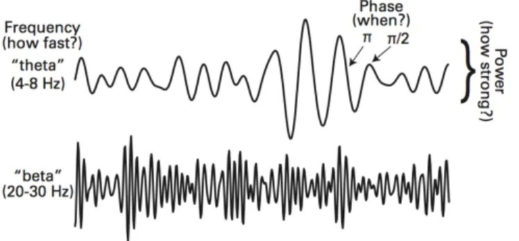
It is worth mentioning that, oscillations are defined by tree information: frequency, power
and phase. Frequency, is the speed of oscillation and its unit is Hertz (Hz), which refers to
the number of cycles per second in radian-base space. The more cycles a signal can round per
second, the faster it is. Moreover, when we are talking about the power of signal, actually,
we are talking about the amount of energy which is the squared amplitude of the oscillations.
Phase, on the other hand, means, where the signal stands in the current moment along the sin
wave (See figure 2.5).
it is possible to obtain the frequency-domain, which is another powerful mathematical tool for
analyzing data.
Figure 2.5: The tree dimensions that show frequency, power and phase (COHEN, 2014)
.
2.2.4
Time-Domain
As it was mentioned, the raw EEG data lives in time-domain, where the changes of
ampli-tude during the time is observable. Ampliampli-tude is convertible to volt (typically microvolt) which
is the measurement of EEG signals(Figure 2.6).
Figure 2.6: Raw EEG data showing oscillation at different speeds and for different lengths of time. Each line corresponds to a specific electrode (SAŁABUN, 2014)
.
There are studies in which the main focus is on time-domain, although the values in this
domain can be difficult to interpret due to the following reasons :
1. Time-domain values may differ depending on data processing and analysis decision.
2. Temporal and spatial filters will change the microvolt values.
3. The results are shown in time-domain are too complicated, not beautiful in analysis
as-pect.
4. When signal is observed in time-domain, values are not periodic. It means it is not
All the given reasons can lead us to get attracted by something more elegant and easier to
un-derstand: the so-called frequency-domain, where the clear results can offer a better environment
to analyze the data and understand the mysteries behind EEG signals.
2.2.5
Frequency-Domain and Fourier Transform
Frequency, means how fast a wave round in radian space. When signals are observed in
frequency-domain, changes in phase or amplitude are measurable. Frequency-domain provides
a better representation of signal. In order to move from time-domain to frequency-domain, a
powerful mathematical tool called Fourier Transform, is utilized. The goal of Fourier analysis
is to express signal in terms of basic sinusoidal components, sine and cosines. By doing so, the
hidden signal properties is accessible. This helps have a better understanding about the signal
(LYONS, 2010). For converting time-domain to frequency-domain, there are tree major types
of Fourier transform as follow :
1. Discrete Fourier Transform (DFT), which maps length-N signals into a set of N discrete
frequency components.
2. Discrete Fourier Series (DFS), which maps N periodic sequence into a set of N discrete
frequency components.
3. Discrete-Time Fourier Transform (DTFT), which maps infinite sequences into a space of
2π-periodic function of real-valued argument.
By sampling EEG data, we can use DFT for moving to frequency-domain. It is possible
to use another algorithm to calculate Fourier transform of a finite-length signal called,
Fast Fourier Transform (FFT), in order to have an algorithm with better performance.
Nevertheless, nowadays computers can use DFT without any problem.
2.2.6
Ways to view Time-Frequency Results
We can imagine time-frequency results as a 3-D cube in which the dimensions are begin
time, frequency and space. Then if we want a 2-D view, we can slice this cube from different
dimensions as follow:
1. Frequency slice (Figure 2.5A): In this case an specific frequency band is selected and the
2. Time slice (Figure 2.5B): What this slice carry out is to show power as a function of
frequency during a period of time.
3. Space slice(Figure 2.5C): Space slice shows data on one time-frequency point over
elec-trodes in a topographical plot.
4. Time-Frequency slice(Figure 2.5D): In time-frequency slice, time is on x-axis and
fre-quency is shown on y-axis. The colors of plot shows various features of signal as though
power,phase clustering and so on.
Figure 2.7: The data cube containing information over time, frequency and space. Since it is difficult to view a 3-D cube, it is sliced in four points of view. (COHEN, 2014)
2.2.7
Brain Frequency Bands
EEG data contains rhythmic activity that reflects neural oscillation. Even in raw EEG data,
this rhythmic activity is observable. The oscillations can be fast, slow or transient. They can also
be changed through the task events. Brain wave frequency bands include delta(2-4 Hz),
theta(4-8 Hz), alpha(theta(4-8-12 Hz), beta(15-30 Hz), lower gamma(30-theta(4-80 Hz) and upper gamma(theta(4-80-150
Hz), however, there is no specific boundary defining these bands. As you might see, theta may
refer to 3-9 Hz, or 3-7 Hz or even 4-7 Hz. Furthermore, individual differences can impact the
frequency-domain with the purpose of using signal filtering techniques to separate each band.
Analyzing the changes in frequency bands, is a way to detect different brain states, like detecting
various stages of sleep.
2.3
Sleep EEG
Sleep is the state of natural rest, which is observable in both humans and animals. It is
also, an interesting but not perfectly known psychological phenomenon. From physical view,
sleep is characterized by reduction in body movement, and decreased reaction for internal or
external stimuli. However all these characteristics are same in unconsciousness state, but they
are technically different (STERIADE, 1992). Sleep is a stage of unconsciousness by which, a
person can be aroused (e.g. sleepwalking and sexual arouse). In this stage the brain is more
responsive for the internal stimuli than external one. Therefore, sleep is distinguishable from all
the other types of deep unconsciousness like coma in which the individual cannot be aroused.
Sleep is necessary for brain to be healthy. Sleep deprivation leads to have lack of
concen-tration. It also causes developing a major decease in memory-related and calculation tasks. The
release of growth hormone in both adults and children takes place during the sleep time.
More-over the body cells show increased production and reduced breakdown during sleep. Therefore,
sleep helps maintaining optimal social and emotional functionality in human being, however,
when it doesn’t takes place in right time and right place, it may cause some problems in form
of sleep diseases and unpleasant accidents during day to day life.
2.3.1
Sleep Stages
There are two distinct states that alternate in cycles and reflect differing levels of neuronal
activity. Each state is characterized by a different type of EEG activity. Sleep consists of
non-rapid eye movement (NREM) and REM sleep ( ˇSU ˇSM ´AKOV ´A, 2004). NREM is further
subdivided into four stages of I (drowsiness), II (light sleep), III (deep sleep), and IV (very deep
sleep).
During the night, NREM and REM stages of sleep alternate. Stages I, II, III, and IV are
followed by REM sleep. A complete sleep cycle, from the beginning of stage I to the end of
REM sleep, usually takes about one and a half hours. However, generally, the ensuing sleep is
relatively short and, for most practical purposes, a duration of 10-30 minutes suffices.
cons-ciousness to unconscons-ciousness stage when the muscles begin to relax. This stage accounts for
5-10% of sleep time. An individual can be easily awaken in this sleep stage. The slow activity
increases as drowsiness get deeper. The findings show that in light drowsiness, the P300
incre-ases in latency and decreincre-ases in amplitude (KOSHINO et al., 1993). Also the interhemispheric
and intrahemispheric EEG coherence alter (WADA et al., 1996). Figure 3.1 shows the EEG
record during drowsiness.
Stage II of sleep occurs throughout the sleep period and represents 40-50% of the total
sleep time. During stage II, brain waves slow down with occasional bursts of rapid waves. Eye
movement stops during this stage. Slow frequencies ranging from 0.7 to 4 cycles/s are usually
predominant; their voltage is high, with a very prominent occipital peak in small children and
gradually fall as age increases (ACHERMANN, 2009).
In stage III, delta waves begin to appear. They are interspersed with smaller, faster waves.
Sleep spindles are still present at approximately 12-14 cycles/s but gradually disappear as the
sleep becomes deeper. In stage IV, delta waves are the primary waves recorded from the brain.
Delta or slow wave sleep (SWS) usually is not seen during routine EEG (MARTIN; MARZEC,
2003). Stages III and IV are often distinguished from each other only by the percentage of delta
activity.
REM sleep includes 20-25% of the total sleep, follows NREM sleep and occurs 45 times
during a normal 8-9 hours sleep period (SIEGEL, 2001). The EEG recorded during REM sleep
is similar to one recorded during wakefulness. Evaluation of REM sleep involves a long waiting
period since the first phase of REM does not appear before 60-90 minutes after the start of sleep.
The EEG in the REM stage shows low voltage activity with a slower rate of alpha.
In general, frequencies from 1 Hz to 16 Hz increase when approaching sleep, while
fre-quencies 17 Hz and higher decrease. This pattern continues after the onset of sleep, except
that power in the 8-11 Hz range begins to increase as well. The change in the 8-11 Hz signal
is especially noticeable in the occipital region where the signal diminishes and transitions to
the frontal lobe. Also in Stage I (that is very important for detecting drowsiness) of sleep the
amplitude of raw EEG signal is low and the signal power in higher frequencies attenuate (HAL
et al., 2014).
2.4
EEG Equipments and Research Costs
At first glimpse, it may seem that EEG research doesn’t cost a lot but this idea comes from
equipments considering EEG caps in various sizes to be used for different head sizes, electrodes
and the other accessories can cost US$ 5000. New amplifiers are expensive too. For university
researches buying the license is also mandatory and the license can coast at least US$ 1200 ,
depending on the EEG cap or headset company. By adding powerful computer, eye tracker and
electrode localization equipment, a BCI research can cost over US$ 15000.
The main problem with EEG and BCI research is that, the more the equipments are precise,
the more research becomes difficult to be implemented in the real life problems. For example,
detecting drowsiness while driving, is hardly possible to be done in a real car using a cap with
128 electrodes, and some computers connected to those electrodes. Another example is using
EEG to control a wheelchair, that can be overwhelming due to the use of too many wires, several
computers and other equipments.
Sometimes the EEG equipments need to be configured and installed by an expert that adds
the configuration and installation cost to the aforesaid equipment expenditure. Furthermore,
there is a main question that may come to mind : How can we apply the results of researches
using huge laboratory equipments, in the real life? It is clear-cut that, we can’t ask the user to
wear an elaborate EEG hat in daily life.
The fact that, elaborate EEG equipments are expensive, not easily configurable and not
possible to be applied in the daily life, imposes this idea of using some equipments that, despite
the less precise data, they are useful enough to be applied in data analysis and development of
BCI applications. This is what leads the researchers to use a new generation of EEG device
calledsingle electrode equipment. Single electrode EEG equipment, comes with lots of defects
which may not be acceptable in advanced research fields, but instead, it totally fits the idea
of having not very accurate, but, good enough data for our needs. These devices are easily
configurable, portable and handy. In the past these devices were not taken seriously, but lately
the number of investigations that use single electrode recording as their main EEG data source,
has been increased. (KATONA et al., 2014).
2.5
Summary
In this chapter, we took a look at the theorical basis of brain computer interface. Various
methods of analyzing EEG signals were reviewed. Afterwards an introduction about sleep EEG
and signals and sleep stages was presented and in the end, we had a look on EEG equipment
and research cost, and we concluded that it seems necessary to use low-cost single electrode
recognizing EEG signals related to wakefulness and drowsiness, the EEG signals should be
classified. To this end, in the next section several well-known classification and feature selection
Chapter 3
C
LASSIFICATION AND FEATURE SELECTION
In this chapter the classification and feature selection algorithms that have been studied in the current research will be explained.
In general, when we talk about classification problems, we tend to go through a decision
making process for future coming data in terms of putting them in predefined and
distinguisha-ble classes, based on already labeled data calledtrainingset. Regarding the drowsiness
detec-tion problem, some researchers have been interested in using machine learning algorithms for
drowsiness detection and several classification methods have been used such as support vector
machine (SVM) and artificial neural networks (ANN). This study, besides surveying the ability
of instance-based learning method for drowsiness detection, aims at comparing the
classifica-tion results obtained by other well-known algorithms with the one obtained by instance-based
approach. Hence, in this chapter, in addition to instance-based learning method, five common
classification algorithms and two feature selection methods are explained.
3.1
Support vector machine (SVM)
Support Vector Machine (SVM) (WESTON; WATKINS, 1998) is a promising method to
classify both linear and non-linear datasets. It uses a non-linear mapping in order to
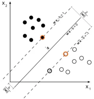
trans-form the data into a higher dimension. The idea is to find the maximum marginal hyperplanes
(MMH) or widest street (SOMAN; LOGANATHAN; AJAY, 2009) between separable areas
among infinite number of separating lines in order to minimizing the classification error. The
area between two separating lines is called plane and the term hyperplane is used to refer to
the decision boundary that we are looking for (HAN; PEI; KAMBER, 2011). The separating
is the offset parameter.
Figure 3.1: SVM finds the widest hyperplane. Support vectors are shown with a red border (XU et al., 2009)
.
Consideringb as an additional weight, the points that are above and under the separating
plane satisfy
yi(w0+w1x1+w2x2) 1,8i. (3.1)
whereyiis +1 if the point is above the hyperplane and -1 when it falls under the hyperplane.
Using Lagrangian formulation the MMH is written as a decision boundary.
d(XT) =
l
∑
i=1
yiαiXiXT +b0 (3.2)
whereXiis support vector,XT is the test tuple andyiis the class label ofith support vector.
Given the test tupleXT, the output tells in which part of the plane the test instance falls. If
the result is a black point, then it falls on the top of plane and belongs to the black class and
in case of being a white, it falls under hyperplane and belongs to white class. When instances
aren’t linearly separable, SVM transforms data to a new dimension in which instances related to
class is characterized by support vectors. Hence, SVM is less prone to over-fitting problem
(HAN; PEI; KAMBER, 2011).
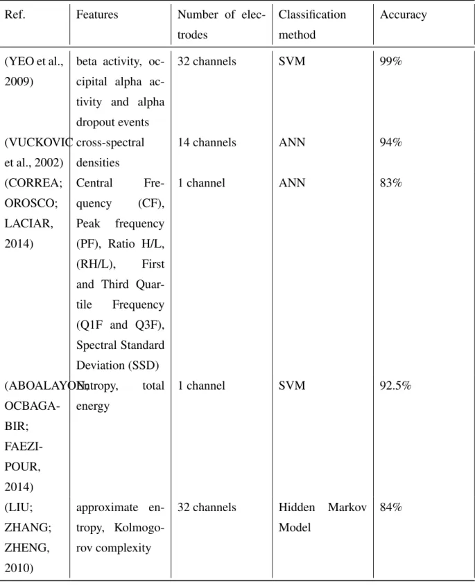
SVM has been used for drowsiness classification in several studies (ABOALAYON;
OC-BAGABIR; FAEZIPOUR, 2014), (YEO et al., 2009). In spite of the fact that SVM is one of
the most powerful classification techniques and it was successfully applied to many real world
problems (LECUN et al., 1995), it has some limitations. Perhaps the biggest problem of support
vector approach is choosing the best kernel function for the given problem (WANG, 2005). The
second drawback of SVM is the speed in both training and test phases (WANG, 2005). Burges
et al. conducted a research to improve the accuracy and speed of support vector machine and
they achieved a factor of fifty speedup in test phase (BURGES; SCHLKOPF, 1997). However,
the training speed is still an unsolved problem (WANG, 2005).
3.2
Naive Bayes
The Naive Bayes (JIAWEI; KAMBER, 2001) is based on the Bayesian theorem and is
particularly suited when the dimensionality of the inputs is high. Naive Bayes can handle an
arbitrary number of independent variables whether continuous or categorical. Given a set of
variables, X ={x1,x2,x3, ...,xd}, we want to construct the posterior probability for the event Cj among a set of possible outcomesCj={c1,c2,c3, ...,cd}. In a more familiar way, X is the predictors andCis the set of categorical levels present in the dependent variable. Using Bayes’
rule:
P(Cj|x1,x2,x3, ...,xd) =P(x1,x2,x3, ...,xn|Cj)⇥P(Cj) (3.3)
whereP(Cj|x1,x2,x3, ...,xd)is the posterior probability of class membership (i.e., the pro-bability that X belongs toCj). Since Naive Bayes assumes that the conditional probabilities of
the independent variables are statistically independent we can decompose the likelihood to a
product of terms:
P(X |Cj) = d
∏
k=1
P(Xk|Cj) (3.4)
and rewrite the posterior as:
P(Cj|X) =P(Cj) d
∏
k=1
P(Xk|Cj) (3.5)
Using the above Bayes’ rule, we label a new case X with a class levelCj that achieves the
Although the assumption that the predictor (independent) variables are independent is not
always accurate, it does simplify the classification task dramatically, because it allows the class
conditional densities P(Xk|Cj) to be calculated separately for each variable, i.e., it reduces a multidimensional task to a number of one-dimensional ones. As a matter of fact, Naive Bayes
reduces a high-dimensional density estimation task to a one-dimensional kernel density
estima-tion. Naive Bayes is simple, easy to implement, robust to noisy data and isn’t very sensitive to
over-fitting problems due to its probabilistic nature.
3.3
Decision tree
A decision tree (QUINLAN, 1987) is a flowchart like tree structure where each nonleaf
node denotes a test on an attribute and each branch represents a result of a test. Each terminal
node holds a class label. The topmost node is the root node. Given a tuple, T, for which the
class is unknown, the attribute values of tuple are tested against the decision tree. The path is
followed from node to leafs where the class prediction for tuple is held. A decision tree works
on two different kind of attributes namely numerical and non-numerical. In case of numeric
attributes, decision trees can be geometrically interpreted as a collection of hyperplanes, each
orthogonal to one of the axes.
Iterative Dichotomiser 3 (ID3) (QUINLAN, 1986) is an algorithm used to generate a
de-cision tree from a dataset. The main choice in ID3 is selecting which attribute to test at each
node in the tree. The idea is to select the attribute that is most useful for classifying instances.
It defines a statistical property calledInformation gainthat measures how well a given attribute
separates the training examples according to their target class. In order to define the
informa-tion gain, it uses a measure of informainforma-tion theory called Entropy. ID3 uses this information
gain measure to select among the candidate attributes at each step while growing the tree.
In general, for constructing a decision tree no knowledge about domain or no parameter
setting is required. Therefore, it is appropriate for exploratory knowledge discovery (HAN; PEI;
KAMBER, 2011). Decision tree can handle high dimensional data. Also, since it represents
the data in tree-like construction, it is appropriate to be assimilated by humans. In general, not
only the learning and classification steps of decision tree induction are simple and fast, also it
has good accuracy. Nevertheless, overfitting is a significant practical difficulty for decision tree
3.4
Logistic regression
The general form of regression, called generalized linear regression (YAN, 2009), assumes
that the data points are coming from a distribution that has a mean that comes from a monotonic
nonlinear transformation of a linear function of the predictors. If we can call this transformation
g, the equation can be written as:
y=g(α+β⇤x) +ε (3.6)
whereα is a constant, sometimes also denoted asb0,β is a vector of the same size as our input
variablexand where the error term isε.
Although the linear regression model is simple and used frequently its not adequate for
some purposes. For example, imagine the response variableY to be a probability that takes on
values between 0 and 1. A linear model has no bounds on what values the response variable
can take, and henceY can take on arbitrary large or small values. However, it is desirable to
bound the response to values between 0 and 1. Also, for linear regression it is hard to describe a
dichotomy outcome with two parallel lines (see Figure 3.2). For this we would need something
more powerful than linear regression.
Figure 3.2: Relationship of a dichotomous outcome variable with a continuous predictor (PENG; LEE; INGERSOLL, 2002)
.
Logistic regression (WALKER; DUNCAN, 1967) solves these kinds of problems using
logit transformation —natural logarithm of odds ratio —to the dependent variable, where odds
logit(Y) =ln(odds) =ln 0
@
eα+βx
1+eα+βx
1 (1+eαe+αβ+xβx)
1
A (3.7)
whereα is theY intercept andβ is the regression coefficient.
Logistic regression is intrinsically simple, it has low variance and so is less prone to
over-fitting. It is also fast and reliable when the dimension gets large (TU, 1996). Another advantage
is that it is easy to inspect.
3.5
Instance-based learning
Instance-based learning (STANFILL; WALTZ, 1986), (ATKESON, 1989) and (MARON;
MOORE, 1993) is an approach including several algorithms that explicitly remembers all the
data that they recieve. They usually have no training time and the computation is performed at
prediction time. This is what seperate this approach from other conventional machine learning
methods where training step occurs between data reception and prediction phases. During the
classification process, this group of methods takes a query point and perform a search on the
database to locate the similar datapoints. Then, it creates a local model such as local average
or local regression so as to predict the output value. There are three main reasons that cause
instance-based approach be prefered over other methods (DENG; MOORE, 1995). These
rea-sons are: a) flexible inductive bias; b) learning parameters does not need to be fixed in advance;
c) instance-based can cover the global local spectrum.
3.5.1
Flexible inductive bias
When the size of instances is little, an algorithm like K-nearest neighbors yields unreliable
prediction, however, as the size of dataset is increased, so the complexity of function that nearest
neighbor can approximate. This is a characteristic with which the approximation power is
increased locally acording to amount of data, that is not observable, for example, by default in
multi-layer neural network.
3.5.2
Learning parameters does not need to be fixed in advance
There are several learning parameters to be configured in instance-based learning. One
suitability. Other parameters include a distance metric (to determine the similarity between
existing datapoints in dataset and a query instance), decision of relevant attributes, decision
about neighbors range and the importance of datapoints based on their approximity to a query
point. Although all of these parameters are configurable, instance-based methods do not need
to decide on them in advance. Hence, they can decide to use a desired default parameter for
one prediction and another different set of parameters for other one. This can be a very useful
feature in autonomous system where it can predict online and at the same time tune the learning
parameters for new coming data (MOORE; HILL; JOHNSON, 1992). In contrast, for
non-instance-based approaches, setting parameters in order to train is necessary. In case of any need
to change one or more parameters, the training phase must be repeated.
3.5.3
Instance-based can cover the global local spectrum
For instance-based methods, it is not necessary to use all the datapoints in feature space to
form a prediction (MOORE; HILL; JOHNSON, 1992). This is specially crucial for noisy
sys-tems where the underlying function is non-linear but generally smooth. In this case,
instance-based methods may use a percentage of nearest datapoints to the query point to form its
predic-tion.
These characteristics make this approach desireable. K-nearest neighbors classification
algorithm is a classical example of instance-based method, in which the k nearest neighbors
of a classifier are used in order to create a local model for the test instance. This algorithm
has been successfully applied to many classification problem (EBRAHIMPOUR; KOUZANI,
2007), (SHI et al., 2011), (DEOLE; LONGADGE, 2014). In the following, this algorithm is
described.
3.5.4
K-nearest neighbors (K-NN)
K-nearest neighbors, also known as proximity search, similarity search or closest point
se-arch, is the most basic instance-based learning algorithm which can be used for both continuous
and discrete values. It assumes that all the instances correspond to a point in the n-dimensional
feature space. This algorithm also considers that if two instances are near to each other, then,
they belong to a same class. For example, if x is an arbitrary instance defined by feature vector
as below:
wherear(x)indicates the value ofrth attribute of x. Therefore the distance is calculated by d(xi, xj) where:
d(xi,xj) = s
n
∑
r=1
(ar(xi) ar(xj))2 (3.9)
Giving labeled training dataset and the above formula, it partitions the feature space to
polygonal-like sections where each polygon contains all the nearest neighbors to a specific
point in feature space.
This algorithm can be refined by giving a weight coefficient based on the distance of each
points to the new instance. Dudani (DUDANI, 1976), first introduced a weighted voting method
for KNN, called the distance-weighted k-nearest neighbor rule (WKNN). In WKNN, the closer
neighbors are weighted more heavily than the farther ones, using the distance-weighted
func-tion. Consequently a neighbor with smaller distance is weighted more heavily than one with
greater.
The K-nearest neighbor algorithm is easily adapted to approximating continuous-valued
target functions. To accomplish this, there is an approach that considers the mean value of the
k nearest training examples rather than calculate their most common value.
In comparison with some classifiers like Support Vector Machine (SVM) and Neural Network
(NN), K-nearest neighbors is simple and easy to implement. Therefore this classifier has been
considered interesting for some researchers who wanted to classify EEG data. Le. et. al. (LI
et al., 2012) used EEG signals to find the study effectiveness in students. They applied Naive
Bayes and K-nearest neighbors to the features extracted from EEG data to find out a
combi-nation, which may mostly contribute to reflect learner’s affect, for example, Attention. They
intended to find a relationship between emotional state and characteristic of brain activity.
Du-ring this investigation they reached the classification rate of 57% using KNN (K=5). They
mentioned that attaining to 57% of correctly classified instances was a good result since they
could find a correlation between emotional state and brain activity while studying. (LI et al.,
2012)
K-NN is a type of instance-based learning algorithm where the function is only locally
approximated. As it was explained, it is the simplest classification algorithm when there is
little or no knowledge about the distribution of data (DEVROYE, 1981). Unlike ANN and
SVM, K-NN has a very fast training, although, its main drawback is running slowly when the
size or dimension of dataset is large. This is because all computation is deferred until
classi-fication which is referred as laziness problem (BHATIA et al., 2010). This algorithm usually