Evaluation of mathematical equations for estimating leaf area in
rapeseed
1Avaliação de equações matemáticas para estimar a área foliar de canola
Genei Antonio Dalmago2*, Cleusa Adriane Menegassi Bianchi3, Samuel Kovaleski4 and Elizandro Fochesatto5
ABSTRACT - The aim of this study was to evaluate estimations of leaf area in rapeseed (Brassica napus L.) and the potential
for application to different genotypes, environmental conditions and types of crop management. In experiments conducted during 2013, 2014, 2016 and 2017, three genotypes of rapeseed, five doses of nitrogen and three sowing dates were used. Leaves were randomly collected from different plants and positions on the plants. The leaf area (LA), and maximum width (W) and length (L) were determined for each leaf, and the product of L and W (LxW) was calculated. Fifty-six equations for estimating LA in rapeseed, where the independent variables were W, L or LxW, were compiled from the bibliography and evaluated in this work. The evaluation was made using the following statistics: significance of the linear (a) and angular (b) coefficients of the regression around the 1:1 line, concordance index (d), bias index (BIAS), mean absolute error (MAE), mean relative error (MRE), random mean squared error (MSEr) and systematic mean squared error (MSEs). Only 11 equations showed the a and b coefficients as not being different from 0 and 1 respectively. However, only 10 were suitable, as they displayed the lowest values for d, BIAS, MAE and RME, and the MSEs was smaller than the MSEr. The MAE ranged from 5.4 cm² to 16.2 cm², well within the error range for generating the equations. LA in rapeseed can be estimated by general biometric equations without considering the specificity of the genotype or the morphological type of the leaf.
Key words: Brassica napus. Colza. Modelling. Leaf area index.
RESUMO - Objetivou-se avaliar a estimativa da área foliar de canola (Brassica napus L.) com potencial de aplicação para
distintos genótipos, condições ambientais e de manejo da cultura. Em experimentos conduzidos em 2013; 2014; 2016 e 2017, utilizou-se três genótipos de canola, cinco doses de nitrogênio e três datas de semeadura. Foram coletadas, aleatoriamente, folhas em diferentes plantas e posições na planta. Em cada folha foi determinada a área foliar (AF), a largura (L) e o comprimento (C) máximos e foi calculado o produto de C e L (CxL). Na bibliografia foram compiladas 56 equações de estimativa da AF para canola, cujas variáveis independentes eram L, C ou CxL, as quais foram avaliadas neste trabalho. A avaliação foi feita pelas estatísticas: significância dos coeficientes linear (a) e angular (b) da regressão em torno da linha 1:1, índice de concordância (d), índice BIAS (BIAS), erro médio absoluto (MAE), erro médio relativo (EMR), erro quadrático médio aleatório (MSEa) e erro quadrático médio sistemático (MSEs). Apenas 11 equações apresentaram os coeficientes a e b não diferentes de 0 e 1, respectivamente. Entretanto, apenas 10 foram adequadas, por apresentarem os menores valores de d, BIAS, MAE, EMR e o MSEs foi menor do que o MSEa. O MAE variou de 5,4 cm² a 16,2 cm², dentro da faixa dos erros da geração das equações. A AF de canola pode ser estimada por equações biométricos gerais sem considerar especificidade de genótipo e/ou tipo morfológico de folha.
Palavras-chave: Brassica napus. Colza. Modelagem. Índice de área foliar.
DOI: 10.5935/1806-6690.20190050 *Author for correspondence
Received for publication 31/07/2018; approved on 17/10/2018
1Pesquisa financiada pela Embrapa, com apoio da FAPERGS, CNPQ e CAPES
2Embrapa Trigo, Rodovia BR 285, km 194, Caixa Postal, 3081, Passo Fundo-RS, Brasil, [email protected] (ORCID ID 0000-0003-0102-3733)
3Departamento de Estudos Agrários, Universidade Regional do Noroeste do Estado do Rio Grande do Sul, Rua do Comércio, 3000, Bairro Universitário, Ijuí-RS, Brasil, [email protected] (ORCID ID 0000-0003-2016-9412)
4Programa de Pós-Graduação em Agronomia, Universidade Federal de Santa Maria, Av. Roraima, 1000, Camobi, Santa Maria-RS, Brasil, [email protected] (ORCID ID 0000-0002-6915-9808)
5Faculdades Integradas do Vale do Iguaçu, Rua Padre Saporiti, 717, União da Vitória-PR, Brasil [email protected] (ORCID ID 0000-0003-0085-034X)
INTRODUCTION
Leaf area (LA) is the principal structure involved in the interception of solar radiation, photosynthesis, evapotranspiration and other plant processes, and has an effect on grain yield (KIRKEGAARD et al., 2012). A precise estimation of LA is therefore fundamental for understanding responses to the environment and to crop management, particularly in rapeseed, since the plant transfers part of the functions of the leaf to the siliquae at the start of the reproductive period (FOCHESATTO
et al., 2016).
Mathematical equations are currently important tools for estimating LA. In general, they relate LA to the dimensional variables of the leaves, such as length (L) and width (W) (LIMA et al., 2012; RICHTER, et al., 2014). There are various equations for estimating LA from the L and W of the leaf, and from the product of these dimensions (CARGNELUTTI FILHO et al., 2015, CHAVARRIA et al., 2011; TARTAGLIA et al., 2016); however, these relationships are not always consistent, neither do they maintain the same response pattern, due to changes that occur in the leaf morphology of rapeseed as a result of such environmental factors as air temperature (STELANOWSKA et al., 1999). This points to the need to evaluate estimating equations for LA in rapeseed, considering the variability of different environments and strategies of crop management.
The representativeness of LA estimates from mathematical equations is another important aspect. According to Chavarria et al. (2011), LA in rapeseed was best estimated from leaf W, but the proposed equation has a relatively low coefficient of determination (R2), which may
lead to imprecise estimates (TARTAGLIA et al., 2016). On the other hand, for Cargnelutti Filho et al. (2015), the best estimate of LA in rapeseed was from leaf L; this was also verified by Tartaglia et al. (2016). However, these authors did not explore the interannual variability of rapeseed growth and development and/or different crop management strategies. In addition, the work of Cargnelutti Filho et al. (2015) and Tartaglia et al. (2016) were carried out in the southern half of the State of Rio Grande do Sul (RS), a region not traditionally used for cultivating rapeseed. As such, there is a need for broader assessments, which would consider the variability of different environmental conditions and types of crop management, applied to the region of greater cultivation, i.e. the north of Rio Grande do Sul.
Furthermore, Cargnelutti Filho et al. (2015) state that specific equations should be sought for each genotype. This contradicts the biological nature of rapeseed: high plasticity with a great ability to compensate for area, and adaptation to different environments (JULLIEN et al., 2011;
KRÜGER et al., 2016). In this context, the hypothesis is that it is possible to find general equations for estimating LA in rapeseed from linear dimensions, including the biological nature and new genotypes that are launched for cultivation in the market (TARTAGLIA et al., 2016).
The aim of this study, therefore, was to evaluate equations for estimating LA in rapeseed with the potential for application to different genotypes, environmental conditions and types of crop management.
MATERIAL AND METHODS
The study was carried out with data collected in the field during 2013, 2014, 2016 and 2017, in the experimental area of Embrapa Trigo, Passo Fundo, RS (28°11’40” S, 52°19’20” W, at an altitude of 713 m). According to the Köppen classification, the region has a type Cfa climate (ALVARES et al., 2013), with soil classified as a humic Dystrophic Red Latosol (STRECK et al., 2008).
The experiments were set up in a randomised block design with four replications, except for 2013, when there were five replications. In 2013 and 2014, the treatments consisted of nitrogen doses (N) of 10, 20, 40, 80 and 160 kg ha-1 as cover fertiliser, using the Hyola
61 genotype, with sowing on 22 April 2013 and 29 April 2014 respectively. For the other years, the experiments were factorial: sowing dates and rapeseed genotypes. There were three sowing dates each year: 18 May 2016, 3 June 2016 and 15 June 2016, and 8 April 2017, 22 May 2017 and 16 June 2017, using the Hyola 61, Diamond and ALHTM6 genotypes.
In 2013 and 2014, sowing was by seeder-fertiliser coupled to a tractor; in 2016 and 2017 sowing was manual with only the base fertiliser added to the soil. The spacing between rows was 34 cm, at a plant density of 40 plants per m2. The base fertilisation and N treatments in the form
of urea, are described in Fochesatto et al. (2016) and Pinto
et al. (2017) for 2013 and 2014. In 2016 and 2017, base
fertilisation followed the same suggestions of Fochesatto
et al. (2016) and Pinto et al. (2017), with 80 kg N ha-1
as cover fertiliser. The other cropping treatments were carried out according to the need of the crop and following suggestions for each specific situation.
LA, W and L were determined during the vegetative phase of the rapeseed, between the end of rosette formation and the end of main stem elongation, from a random sampling of leaves from different plants in the plot and different positions on the plants. In 2013, two leaves were sampled per plot, giving a total of 50 leaves; in 2014 nine leaves were sampled per plot, totalling 180 leaves, and in 2016 and 2017 four and five leaves were sampled per plot,
for a total of 144 and 180 leaves respectively. Nine leaves were discarded due to damage during the transportation and handling of the plant material. This generated a series of 546 independent observations representative of the main causes of variability in the rapeseed canopy.
A LICOR model 3100-L optical planimeter was used to determine the individual LA of each leaf. The maximum linear dimensions for leaf L and W were determined by ruler. The L was measured along the central vein, starting from the insertion of the petiole in the plant to the apex of the leaf, and the maximum W was measured across the central part of the leaf blade. The product LxW was then calculated.
The data were evaluated using descriptive statistics: minimum, mean, median, maximum, standard deviation, coefficient of variation (CV), kurtosis and asymmetry, with data normality verified by means of the Kolmogorov-Smirnov test (KS). In addition, LA dispersion profiles were generated as a function of L, W and LxW to verify the distribution pattern of the data.
The equations for estimating LA in the rapeseed were compiled from Chavarria et al. (2011), Cargnelutti Filho et al. (2015) and Tartaglia et al. (2016), for the Hyola 61, Hyola 433, Hyola 76, Hyola 411 and Hyola 420 genotypes. In all, 56 equations were studied, being at present the only equations available for the growing conditions in the south of Brazil. The equations under study were generated based on linear, quadratic and power models.
To meet the objectives of the study, the data for LA, W, L and LxW were grouped into six distinct sets of data, representing the six distinct conditions for variability. The first set involved all the data from the experiments in 2013, 2014, 2016 and 2017, irrespective of genotype and N treatment (TD). The second was composed of all the TD, but minus the extreme N treatments (10, 20 and 160 kg ha-1) of
2013 and 2014 (TDMN), i.e. keeping only treatments within the range normally used for N as cover fertiliser in rapeseed (between 40 and 80 kg N ha-1). The third, fourth, fifth and
sixth sets of data comprised the following: H61 - all the data for the Hyola 61 genotype from the four experiments; H61MN – the same data as H61, but minus the extreme N treatments (10, 20 and 160 kg ha-1); Diam - data for the
Diamond genotype from the 2016 and 2017 experiments; and M6 – data for the ALHTM6 genotype from 2016 and 2017.
The performance of the equations for accuracy and precision of the estimates was evaluated by different statistics (WILLMOTT et al., 1985), assuming that to be considered suitable, the equations should meet the criteria of all the statistics used. First, data dispersion around the 1:1 line was evaluated, considering the observed
(measured) values along the ordinate and the simulated (estimated) values along the abscissa (PIÑEIRO et al., 2008), as per equation 1.
Oi = a + bSi (1) where: Oi is the observed (measured) value, Si is the value simulated by the model as a function of the leaf dimensions (W, L and LxW), and a and b are the angular and linear coefficients of the regression line respectively. The coefficients, a and b, were tested by t-test at 5% probability of error as to the significance of their variation relative to 0 and 1 respectively. The ideal model is one in which coefficient a does not differ from 0 and coefficient
b does not differ from 1 (SMITH; ROSE, 1995).
Data dispersion around the 1:1 line was complemented (PIÑEIRO et al., 2008) by the following statistics: concordance index (d), BIAS index, mean absolute error (MAE), mean relative error (MRE), random mean squared error (MSEr) and systematic mean squared error (MSEs).
For the bias index, which is the mean value of the deviations of the simulated values in relation to the observed values, the calculation was adapted from Leite and Andrade (2002) as per equation 2:
BIAS = (ƩSi - ƩOi)/ƩOi (2) where: Oi is the observed (measured) value and Si is the value simulated by the model as a function of the leaf dimensions (W, L and LxW). The bias index shows the trend of the model, where the closer the value is to zero, the lower the trend and the better the model.
The concordance index d is the statistic that evaluates the degree to which the simulations are free of error, and represents the accuracy of the model. This varies from 0, where there is no agreement, to 1, where there is perfect agreement between the observed and simulated values; d was calculated as perWillmott et al. (1985), from equation 3:
(3) where: Si is the simulated value, Oi is the observed value and ō is the mean of the observed values.
The MAE, which is the mean of the absolute values of the errors was calculated as per Willmott and Matsuura (2005), with equation 4:
MAE = [Σ(|Oi - Si|)]/n (4) where: Oi is the observed value, Si is the simulated value and n is the number of observations. The MAE considers
the magnitude of the errors, assigning the same weight to all the residuals, and is considered a robust indicator (FOX, 1981), as it is less affected by outliers and is recommended for evaluating equations (WILLMOTT; MATSUURA, 2005).
For the MRE, which is used to verify the margin of error in estimating the model, Equation 5 was used: MRE = 100{Σ[|Oi - Si|)/Oi]}/n (5) where: Oi is the observed value, Si is the simulated value and n is the number of observations. The coefficient 100 transforms the values into a percentage.
The random (MSEr) and systematic (MSEs) parts of the mean squared error were calculated from equations 6 and 7 respectively, as per Willmott (1982):
MSEr = [Σ(Ŝi - Si)2]/n (6)
MSES = [Σ(Ŝi- Oi)2]/n (7) where:
Ŝi = a + bOi (8) with a and b the linear and angular coefficients of the regression line equation between the simulated and observed values. MSEr represents the random variations of the measurements and is due to uncontrolled factors affecting each measurement differently, whereas MSEs represents the difference between the measured value and the true value, and is the same for the total measurement.
The calculations were carried out on spreadsheets using the Excel® software. For the statistical analysis, the
R software (R CORE TEAM, 2018) was used.
RESULTS AND DISCUSSION
In general, the values for the leaf dimensions L and W varied between 3.6 and 46.5 cm and between 2.0 and 20.5 cm respectively, while the product LxW and LA varied between 7.2 and 672.4 and between 3.7 and 461.1 respectively (Table 1). These limits are within or fairly close to those presented by Chavarria et al. (2011), Cargnelutti Filho et al. (2015) and Tartaglia et al. (2016) for obtaining the equations. Variations in the limits of the independent variables (L, W, LxW) and in LA were found between the sets of data, and were due to variability between genotypes and the effect of nitrogen fertilisation. On average, the H61 and H61MN genotype had longer and wider leaves than Diam and M6. A rise in N cover fertilisation increased this difference (Table 1). It is therefore evident that variations in sowing
times (NANDA; BHARGAVA; RAWSON, 1995), environmental conditions (STELANOWSKA et al., 1999) and N fertilisation (BOUCHET et al., 2016) affect the leaf morphology in rapeseed.
The experimental strategy adopted, involving some of the main factors of rapeseed management, different environmental conditions (different years of cultivation) and genotypes of a different genetic base, guaranteed the desired variability, necessary for evaluating the equations (Table 1). The CV ranged from 21.1% to 114.6%, being approximately twice as much for LxW and LA as for leaf L and W, as found by Cargnelutti Filho et al. (2015). Among the sets of data, the CV was higher in M6, not only for all the independent variables, but also for LA, whereas for the H61, H61MN and Diam data sets, the values for CV were close (Table 1). This is an indicator that justifies the search for more robust equations which consider variability in the LA of the crop (Table 1).
In the data set for most of the variables (L, W, LxW and LA), asymmetry and kurtosis were not significant. Leaf W showed more situations with significant asymmetry. However, as the significant values for asymmetry were low (≤ 0.73) and positive, similar to those found by Cargnelutti Filho et al. (2015), this indicates a slight departure from normality. In the vast majority of the situations under study, the p-values of the KS-test were less than p = 0.05, proving this slight departure from normality. However, the statistical indices together (kurtosis, asymmetry and p-value) indicate a small departure from normality for L and W, compared to LxW and LA, as found by Cargnelutti Filho
et al. (2015), particularly for TD, TDMN, H61 and H61MN, in contrast to a greater departure for M6. This response is also verified by the magnitude of the difference between the mean and the median, which is lower for L and W than for LxW and LA in each of the experimental situations (Table 1). According to Cargnelutti Filho et al. (2015), such statistical characteristics are suitable for validating equations.
The data dispersion (Figure 1) indicated patterns already expected for rapeseed (CARGNELUTTI FILHO
et al., 2015; CHAVARRIA et al., 2011; TARTAGLIA et al., 2016), where LA has a non-linear relationship to
the leaf L and W (Figures 1a to 1f) and a linear pattern for LxW (Figures 1g to 1i). This was also found in other species, such as the jack bean (TOEBE et al., 2012) and the forage turnip (CARGNELUTTI FILHO et al., 2012). The dispersion was greater when LA was a function of L, followed by LxW and W (Figure 1), indicating a probable better response for equations using W as an independent variable.
An analysis of the significance of the a and b coefficients of the regression between the measured and
Table 1 - Number of leaves (n), values: minimum (Mn), mean (M), median (MD), maximum (Mx), standard deviation (SD), coefficient
of variation (CV), kurtosis (K), asymmetry (A) and p-value in the Kolmogorov-Smirnov test [KS(p)] for length (L), width (W), the product of length x width (LxW) of the leaf blade, and leaf area (LA) in three rapeseed (Brassica napus L.) genotypes and/or for different years of evaluation and for the complete set of data
*Kurtosis or asymmetry differ from zero by t-test at 5% probability of error.nsKurtosis or asymmetry differ from zero by t-test at 5% probability of error
Data set Statistic
n Mn M MD Mx SD CV(%) K A KS(p)
L – Length of the leaf blade (cm)
TD 546 3.6 18.2 17.5 46.5 7.7 42.2 -0.41ns 0.40ns 0.028 TDMN 408 3.6 17.0 15.9 46.5 7.7 45.4 0.05ns 0.65ns 0.006 H61 336 3.6 20.3 20.2 37.0 7.1 35.1 -0.76ns 0.10ns 0.273 H61MN 198 3.6 19.1 18.5 37.0 7.4 38.9 -0.67ns 0.27ns 0.329 Diam 105 4.0 14.9 14.0 29.0 5.7 37.8 -0.53ns 0.41ns 0.422 M6 105 4.3 15.0 12.5 46.5 8.9 59.6 1.36ns 1.28ns 0.040
W – Width of the leaf blade (cm)
TD 546 2.0 8.4 7.7 20.5 3.6 42.3 -0.11ns 0.58 <0.001 TDMN 408 2.0 7.7 7.0 20.5 3.3 43.5 0.71* 0.82* 0.007 H61 336 2.0 9.5 9.2 20.5 3.6 37.8 -0.28ns 0.43* 0.024 H61MN 198 2.0 8.6 8.2 20.5 3.5 41.0 0.54* 0.73* 0.010 Diam 105 2.1 6.9 6.8 14.5 2.5 35.5 0.18ns 0.57* 0.669 M6 105 2.1 6.6 6.0 15.3 3.2 48.3 -0.02ns 0.83* 0.118
LxW – Product of the length and width of the leaf blade (cm²)
TD 546 7.2 178.0 136.2 672.4 137.5 77.3 0.57ns 1.06ns <0.001 TDMN 408 7.2 153.0 114.2 672.4 129.2 84.4 0.73ns 1.08ns <0.001 H61 336 7.2 214.0 185.0 672.4 140.1 65.5 -0.11ns 0.76ns 0.003 H61MN 198 7.2 187.8 148.0 672.4 137.8 73.4 0.73ns 1.08ns 0.007 Diam 105 8.4 116.2 93.8 420.5 81.2 69.9 1.23ns 1.15ns 0.010 M6 105 11.4 124.3 71.4 660.3 135.1 108.7 3.58ns 1.91ns <0.001 LA – Leaf area (cm²) TD 546 3.7 90.6 66.8 461.1 75.0 82.8 2.05ns 1.35ns <0.001 TDMN 408 3.7 76.1 54.6 461.1 69.2 91.0 3.75ns 1.67ns <0.001 H61 336 4.2 214.0 185.0 461.1 140.1 65.5 -0.11ns 0.76ns 0.001 H61MN 198 4.2 95.9 75.5 461.1 79.8 83.2 3.75ns 1.67ns 0.003 Diam 105 3.7 58.1 45.3 214.6 42.4 73.0 1.49ns 1.21ns 0.066 M6 105 4.9 56.8 35.1 260.5 58.7 103.4 2.64ns 1.73ns <0.001
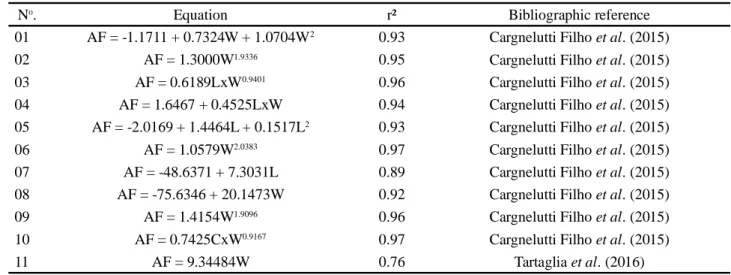
estimated LA revealed the high accuracy for estimating LA in rapeseed of equations 01, 02, 03, 04, 05, 06, 07, 08, 09, 10 and 11 (Table 2) for at least one of the sets of data. These equations met the desired statistical assumption, which is to show, at the same time, the a and
b coefficients as not different from 0 or 1 respectively
(Table 3), demonstrating a broad and more general application potential. The selected equations were obtained by Cargnelutti Filho et al. (2015) specifically
for the Hyola 61 (4 equations), Hyola 76 (3 equations) and Hyola 433 (2 equations) genotypes. Only one of the equations obtained by Tartaglia et al. (2016) was suitable, being generated for the set of oval-shaped leaves collected from the Hyola 61, Hyola, 433, Hyola 420 and Hyola 411 hybrids and represented by the number 11 (Table 3). The other equations generated by Cargnelutti Filho et al. (2015) and Tartaglia et al. (2016), and those generated by Chavarria et al. (2011), showed the a and b coefficients as
Figure 1 - Leaf area dispersion in rapeseed (Brassica napus L.) as a function of length and width, and the product of length x
width, in leaves of the Hyola 61 (H61 and H61MN), Diamond (Diam) and ALHTM6 (M6) genotypes and for the complete set of data (TD and TDMN). (NOTE: MN in subscript means no extreme doses of nitrogen as cover fertiliser in the T1, T2 and T5 treatments for 2013 and 2014)
Table 2 - Equations for estimating leaf area (LA) from leaf length (L) and width (W), and the product of length x width (LxW)
in rapeseed (Brassica napus L.), with the respective coefficients of determination (r²) and the bibliographic reference to where the equation was obtained
No. Equation r² Bibliographic reference
01 AF = -1.1711 + 0.7324W + 1.0704W2 0.93 Cargnelutti Filho et al. (2015)
02 AF = 1.3000W1.9336 0.95 Cargnelutti Filho et al. (2015)
03 AF = 0.6189LxW0.9401 0.96 Cargnelutti Filho et al. (2015)
04 AF = 1.6467 + 0.4525LxW 0.94 Cargnelutti Filho et al. (2015) 05 AF = -2.0169 + 1.4464L + 0.1517L2 0.93 Cargnelutti Filho et al. (2015)
06 AF = 1.0579W2.0383 0.97 Cargnelutti Filho et al. (2015)
07 AF = -48.6371 + 7.3031L 0.89 Cargnelutti Filho et al. (2015) 08 AF = -75.6346 + 20.1473W 0.92 Cargnelutti Filho et al. (2015)
09 AF = 1.4154W1.9096 0.96 Cargnelutti Filho et al. (2015)
10 AF = 0.7425CxW0.9167 0.97 Cargnelutti Filho et al. (2015)
Table 3 - Linear (a) and angular (b) coefficients of the regression equation between the measured leaf area and that estimated by the
equations for six sets of data: the complete set of data (TD), the complete set of data minus the data from the extreme N treatments (10, 20 and 160 kg ha-1) in 2013 and 2014 (TD
MN), all the Hyola 61 (H61) genotype data, all the Hyola 61 genotype data, minus the
data from the extreme nitrogen treatments (10, 20 and 160 kg ha-1) in 2013 and 2014 (H61
MN), the Diamond (Diam) genotype and the
ALHTM6 (M6) genotype Equation Number Data set TD TDMN H61 H61MN Diam M6 Linear coefficient - a 01 -0.19ns -1.92ns 2.03ns -0.16ns -1.55ns -4.45* 02 -1.37ns -3.03* 0.59ns -1.57ns -2.25ns -5.17* 03 -8.41* -7.79* -12.45* -14.48* -5.59* 0.07ns 04 -5.16* -5.01* -8.14* -10.73* -3.96* 1.96ns 05 -3.56ns -2.92ns -8.22ns -11.54* -7.31* 4.53ns 06 3.37* 1.46ns 6.19* 3.87* 1.01ns -2.07ns 07 -8.01* -5.03ns -18.48* -16.92* -0.48ns 4.28ns 08 -3.98* -1.45ns -12.06* -9.58* 5.41* 7.40* 09 -2.52* -4.12* -0.77ns -2.89ns -3.05ns -5.93* 10 -10.64* -9.81* -15.17* -16.97* -7.12* -1.44ns 11 7.04ns -2.71ns 31.62* 7.02ns 20.53ns -7.60ns Angular coefficient - b 01 0.96ns 0.99* 0.95ns 0.98* 0.97* 1.02* 02 0.99* 1.02* 0.98* 1.01* 0.99* 1.04ns 03 1.25ns 1.22ns 1.30ns 1.32ns 1.19ns 1.01* 04 1.24ns 1.22ns 1.29ns 1.31ns 1.22ns 1.01* 05 1.12ns 1.05* 1.22ns 1.21ns 1.12ns 0.80ns 06 0.90ns 0.93ns 0.89ns 0.91ns 0.92ns 0.97* 07 1.17ns 1.08ns 1.30ns 1.24ns 0.97* 0.87ns 08 1.01* 0.99* 1.08ns 1.07ns 0.83ns 0.88ns 09 0.98ns 1.00* 0.97ns 0.99* 0.97* 1.02* 10 1.21ns 1.18ns 1.27ns 1.28ns 1.14ns 0.98* 11 1.07* 1.08* 0.90* 1.07* 0.58ns 1.05*
nsLinear coefficient does not differ from 0 by t-test at 5% probability of error;*Angular coefficient does not differ from 1 by t-test at 5% probability of error
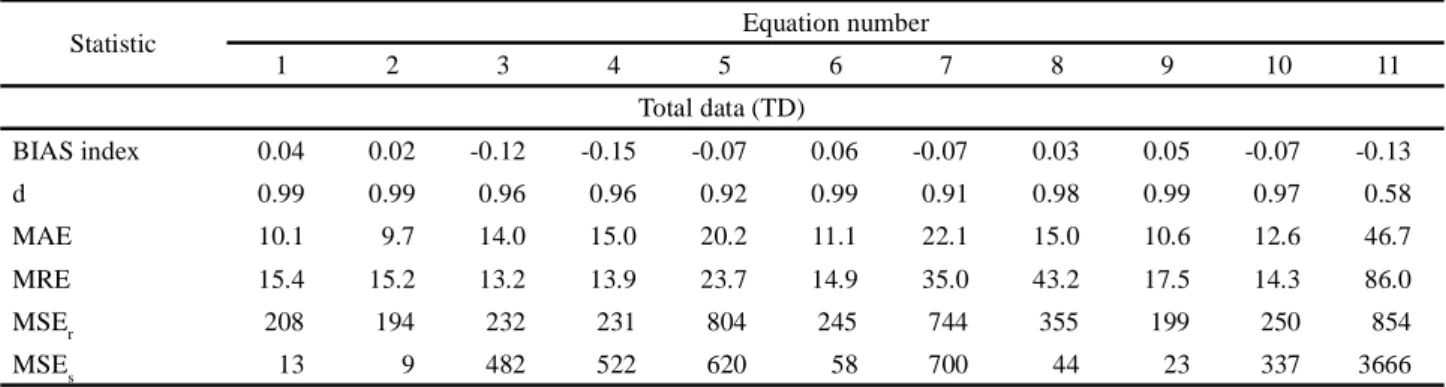
Table 4 - Bias Index (BIAS), concordance index (d), mean absolute error (MAE), mean relative error (MRE), random mean squared
error (MSEr) and systematic mean squared error (MSEs) associated with evaluation of the equations for estimating leaf area in rapeseed (Brassica napus L.) for six sets of data of differing variability
Statistic Equation number
1 2 3 4 5 6 7 8 9 10 11 Total data (TD) BIAS index 0.04 0.02 -0.12 -0.15 -0.07 0.06 -0.07 0.03 0.05 -0.07 -0.13 d 0.99 0.99 0.96 0.96 0.92 0.99 0.91 0.98 0.99 0.97 0.58 MAE 10.1 9.7 14.0 15.0 20.2 11.1 22.1 15.0 10.6 12.6 46.7 MRE 15.4 15.2 13.2 13.9 23.7 14.9 35.0 43.2 17.5 14.3 86.0 MSEr 208 194 232 231 804 245 744 355 199 250 854 MSEs 13 9 482 522 620 58 700 44 23 337 3666
significantly different from 0 and 1 (data not shown), and were therefore not suitable.
Most of the selected equations (Table 3) have W as an independent variable, while the others have LxW (2 equations) or L (2 equations). These results indicate that W is the most suitable variable for estimating LA in rapeseed, and equations that use this independent variable therefore tend to have better performance, as previously pointed out by Cargnelutti Filho et al. (2015) and Tartaglia
et al. (2016). Leaf W was also the best performing variable
in estimating LA in the sunflower (MALDANER et al., 2009), Bergenia purpurascens (ZHANG; LIU, 2010) and Italian courgette (FIALHO et al., 2011), possibly because W maintains constant shape during LA growth and development (MISLE et al., 2013).
Another important aspect found in evaluating the
a and b coefficients was the suitability of the equations
for the Diamond and ALHTM6 genotypes, despite having TD minus the extreme nitrogen treatment (TDMN)
BIAS index 0.04 0.02 -0.10 -0.12 -0.01 0.06 -0.01 0.03 0.05 -0.04 -0.20 d 0.99 0.99 0.96 0.96 0.93 0.99 0.92 0.98 0.99 0.97 0.50 MAE 9.2 9.0 10.7 11.5 16.2 9.6 18.3 15.1 9.8 10.1 46.8 MRE 17.3 17.2 12.7 13.1 24.6 16.2 38.6 52.9 19.8 14.9 101.4 MSEr 176 164 211 207 761 205 728 384 169 229 1170 MSEs 11 16 323 351 342 25 394 32 24 225 3811
Data for the Hyola 61 genotype (H61)
BIAS index 0.03 0.01 -0.15 -0.17 -0.12 0.06 -0.10 0.03 0.04 -0.10 -0.21 d 0.99 0.99 0.94 0.94 0.88 0.99 0.87 0.98 0.99 0.95 0.52 MAE 11.8 11.3 18.8 20.0 26.2 13.4 28.4 15.5 12.1 16.7 55.2 MRE 13.1 12.7 14.1 15.0 23.5 13.4 30.0 28.6 14.4 14.2 66.3 MSEr 272 253 274 275 843 323 759 337 258 294 964 MSEs 14 5 822 869 1236 93 1412 121 21 605 5066
H61 minus the extreme nitrogen treatment (H61MN)
BIAS index 0.02 0.01 -0.13 -0.15 -0.07 0.05 -0.05 0.02 0.04 -0.08 -0.39 d 0.99 0.99 0.95 0.95 0.89 0.99 0.88 0.98 0.99 0.96 0.48 MAE 11.1 10.9 15.5 16.3 22.3 12.0 25.0 16.0 11.6 14.3 61.3 MRE 15.3 15.1 13.7 14.0 25.1 15.0 33.9 38.4 17.1 15.2 84.3 MSEr 255 237 267 260 853 302 837 401 242 290 1764 MSEs 8 15 725 756 1018 40 1177 133 19 554 6262
Diamond genotype (Diam)
BIAS index 0.06 0.05 -0.08 -0.12 0.00 0.06 0.04 0.10 0.09 -0.02 0.10 d 0.99 0.99 0.98 0.98 0.97 0.98 0.97 0.97 0.98 0.99 0.52 MAE 6.9 6.6 6.9 8.1 8.5 7.0 10.6 12.5 7.6 5.9 32.2 MRE 16.8 16.7 12.4 13.5 19.8 15.6 32.5 46.5 19.8 13.6 110.2 MSEr 92 87 27 25 110 104 188 177 90 30 537 MSEs 13 11 79 117 61 15 18 60 26 38 1255 ALHTM6 genotype (M6) BIAS index 0.06 0.05 -0.01 -0.04 0.15 0.07 0.07 -0.01 0.08 0.05 0.06 d 0.98 0.98 0.99 0.98 0.95 0.98 0.96 0.95 0.98 0.99 0.52 MAE 7.9 7.9 5.4 5.7 12.5 7.5 13.5 15.9 8.7 6.2 35.2 MRE 21.4 21.5 10.9 10.9 28.3 19.0 53.6 86.6 25.1 15.5 122.2 MSEr 107 103 92 101 444 115 326 368 109 96 675 MSEs 20 26 6 10 141 15 28 4 31 8 1828 Continued Table 4
been obtained for the Hyola 61, Hyola 76 and Hyola 433 genotypes, or even for oval-shaped leaves (Table 3). In the case of the ALHTM6 genotype, the number of suitable equations was greater than for the other genotypes, or when all the data were used together. However, for the Diamond genotype, the number of equations was equal to that of the Hyola 61 genotype, with most of the equations being the same (equations 02, 05 and 09). Furthermore, it was found that for the TDMN and H61MN data sets, the number of equations was higher than for TD and H61 (Table 3). This response indicates that management factors may affect the estimation of LA in rapeseed, as they affect leaf morphology. On the other hand, since there were equations that fit each set of data (TD, TDMN, H61, H61MN, Diam and M6), they prove the hypothesis of more general equations for estimating LA in rapeseed, without the specificity indicated by Cargnelutti Filho et al. (2015) and/or by Tartaglia et al. (2016) being necessary.
Additional analysis for data dispersion relative to the 1:1 line suggested by Piñeiro et al. (2008), was only carried out for equations that met the significance of the a and b coefficients (01, 02, 03, 04, 05, 06, 07, 08, 09, 10 and 11) for at least one set of evaluated data (Table 4). This strategy was adopted, since the other equations are susceptible to significant error.
In general, the selected equations also presented other favourable evaluation statistics, except for equation 11, which had the most distant values in relation to the other equations (Table 4). This equation will be presented and discussed separately.
Equations 01, 02, 03, 04, 05, 06, 07, 08, 09 and 10 presented values for BIAS close to zero in the different sets of data under evaluation (-0.04 ≤ BIAS ≤ 0.09), indicating that there were no under or overestimates. The accuracy of these equations is also confirmed by the d index, where the majority had a value equal to 0.99 (0.93 ≤ d ≤ 0.99). Such a condition indicates good similarity between the measured and estimated values for LA (Table 4).
The MAE associated with the LA estimates ranged from 5.4 cm2 to 16.2 cm2, and were within the range of
errors found by Cargnelutti Filho et al. (2015) and Tartaglia
et al. (2016) when obtaining the equations for other
environments, management conditions and/or genotypes. The similarity of the values for MAE in the present study, in relation to those found by Cargnelutti Filho et al. (2015) and Tartaglia et al. (2016), is another good indicator of the estimating power of the selected equations for LA in rapeseed under different environmental and management conditions. When the analysis was carried out by comparing the sets of data, it was found that although the number of equations was greater for the TDMN and H61MN data sets, on average, the MAE increased (TDMN) or did
not change (H61MN) in relation to the TD and H61 data sets respectively. Overall, however, the MRE increased by 16.4 and 3.1 percentage points respectively under this condition (Table 4).
Another important aspect to be noted in this study is the suitability of the equations for the Diamond and ALHTM6 genotypes (Table 4). In addition to there being a greater number of suitable equations for these two genotypes compared to the other sets of data, the values for MAE were generally less than those seen for H61, H61MN, TD and TDMN (5.4 ≤ MAE ≤ 11.6). On the other hand, the mean value for MRE among the equations for the Diamond and ALHTM6 genotypes increased in relation to the equations evaluated for the TD TDMN, H61 and H61MN sets of data (Table 4), but not so as to compromise their application. The suitability of the equations generated for genotypes with a different genetic base (Diamond and ALHTM6) is a robust indicator, which helps in proving the hypothesis of this work.
A breakdown of the errors associated with the estimations made by the equations (01, 02, 03, 04, 05, 06, 07, 08, 09, 10) also corroborates their indication as the most suitable for estimating LA in rapeseed using L and W, or LxW (Table 4). As can be seen, all the selected equations showed the MSEs as less than the MSEr. This is a desired condition when evaluating equations, as it shows that the equation is free from any bias associated with the measured data and/or generation of the equations (WILLMOTT et al., 1985).
In relation to equation 11, despite the a and b coefficients not being different to 0 and 1 respectively (Table 3), the equation did not meet the other statistics of performance evaluation (Table 4). This equation had the largest deviations between the selected equations for each data set to which it was applied, with the exception of M6. In addition, the d index was one of the lowest among all the equations (Table 4), with the MAE and MRE being among the highest. However, the statistic that made equation 11 unsuitable for estimating LA in rapeseed was the MSEs, which was higher than the MSEr for each set of data (Table 4). As such, the equations presented by Tartaglia et al. (2016) were not sufficiently suitable for estimating LA in rapeseed from the leaf dimensions of W and L or LxW, outside the conditions in which they were obtained.
In general, equations 02, 05 and 09 proved to be more suitable for estimating LA in rapeseed, and should be used, as they deal with variability related to genetic diversity and factors of crop management. As such, the hypothesis that LA in rapeseed can be estimated by general equations is confirmed, where the linear dimensions of W and L or LxW are taken as independent variables.
CONCLUSION
Leaf area in rapeseed is adequately estimated by general biometric equations for different genotypes, conditions of nitrogen cover and sowing times, as they do not maintain any specificity regarding genotype and/or leaf morphology.
ACKNOWLEDGEMENTS
The authors wish to thank the agricultural technician of Embrapa Trigo, Elisson Stephanio Savi Pauletti, and field assistant, Cristian Maicol Plentz, for their help in collecting the data. Thanks also go to the Fundação de Amparo à Pesquisa do Rio Grande do Sul (FAPERGS), to the Conselho Nacional Desenvolvimento Científico e Tecnológico (CNPq) and the Coordenação de Aperfeiçoamento de Pessoas de Nível Superior (CAPES) for the master’s and research productivity scholarships.
REFERENCES
ALVARES, C. A. et al. Köppen’s climate classification map for Brazil. Meteorologische Zeitschrift, v. 22, n. 6, p. 711-728, 2013.
BOUCHET, A. S. et al. Nitrogen use efficiency in rapeseed: a review. Agronomy for Sustainable Development, v. 36, n. 38, p. 1-20, 2016.
CARGNELUTTI FILHO, A. et al. Estimação da área foliar de canola por dimensões foliares. Bragantia, v. 74, n. 2, p. 139-148, 2015.
CARGNELUTTI FILHO, A. et al. Estimativa da área foliar de nabo forrageiro em função de dimensões foliares. Bragantia, v. 71, n. 1, p. 47-51, 2012.
CHAVARRIA, G. et al. Índice de área foliar em canola cultivada sob variações de espaçamento e de densidade de semeadura.
Ciência Rural, v. 41, n. 12, p. 2084-2089, 2011.
FIALHO, G. S. et al. Predição da área foliar em abobrinha-italiana: um método não destrutivo, exato, simples, rápido e prático. Revista Brasileira de Agropecuária Sustentável, v. 1, n. 2, p. 59-63, 2011.
FOCHESATTO, E. et al. Interception of solar radiation by the reproductive structures of canola hybrids. Ciência Rural, v. 46, n. 10, p. 1790-1796, 2016.
FOX, D. G. Judging air quality model performance. Bulletin of
the American Meteorological Society, v. 62, n. 5, p. 599-609,
1981.
JULLIEN, A. et al. Characterization of the interactions between architecture and source–sink relationships in winter oilseed rape (Brassica napus) using the Green Lab model. Annals of Botany, v. 107, n. 5, p. 765-779, 2011.
KIRKEGAARD, J. A. et al. Physiological response of spring canola (Brassica napus) to defoliation in diverse environments.
Field Crops Research, v. 125, n. 18, p. 61-68, 2012.
KRÜGER, C. A. M. B. et al. Rapeseed population arrangement defined by adaptability and stability parameters. Revista
Brasileira de Engenharia Agrícola e Ambiental, v. 20, n. 1,
p. 36-41, 2016.
LEITE, H. G.; ANDRADE, V. C. L. Um método para condução de inventários florestais sem o uso de equações volumétricas.
Revista Árvore, v. 26, n. 3, p. 321-328, 2002.
LIMA, R. T. de et al. Modelos para estimativa da área foliar da mangueira utilizando medidas lineares. Revista Brasileira de
Fruticultura, v. 34, n. 4, p. 974-980, 2012.
MALDANER, I. C. et al. Modelos de determinação não-destrutiva da área foliar em girassol. Ciência Rural, v. 39, n. 5, p. 1356-1361, 2009.
MISLE, E. et al. Leaf area estimation in muskmelon by allometry. Photosynthetica, v. 51, n. 4, p. 613-620, 2013. NANDA, R.; BHARGAVA, S. C.; RAWSON, H. M. Effect of sowing date on rates of leaf appearance, final leaf numbers and areas in Brassica campestris, B. juncea, B. napus and B. carinata.
Field Crops Research, v. 2, n. 2/3, p. 125-134, 1995.
PIÑEIRO, G. et al. How to evaluate models: observed vs. predicted or predicted vs. observed? Ecological Modelling, v. 216, n. 3/4, p. 316-322, 2008.
PINTO, D. G. et al. Correlations between spectral and biophysical data obtained in canola canopy cultivated in the subtropical region of Brazil. Pesquisa Agropecuária
Brasileira, v. 52, n. 10, p. 825-832, 2017.
R CORE TEAM. R: a language and environment for statistical computing. Vienna, Austria: R Foundation for Statistical Computing, 2018. Disponível em: <https://www.R-project. org/.>. Acesso em: 04 out. 2018.
RICHTER, G. L. et al. Estimativa da área de folhas de cultivares antigas e modernas de soja por método não destrutivo. Bragantia, v. 73, n. 4, p. 416-425, 2014.
SMITH, E. P.; ROSE, K. A. Model goodness-of-fit analysis using regression and related techniques. Ecological Modelling, v. 77, n. 1, p. 49-64, 1995.
STEFANOWSKA, M. et al. Low temperature affects pattern of leaf growth and structure of cell walls in winter oilseed rape (Brassica napus L., var. oleifera L.). Annals of Botany, v. 84, n. 3, p. 313-319, 1999.
STRECK, E. V. et al. Solos do Rio Grande do Sul. 2. ed. Porto Alegre: EMATER/RS - ASCAR, 2008. 220 p.
TARTAGLIA, F. de L. et al. Modelos não destrutivos para determinação da área foliar em canola. Revista Brasileira de
Engenharia Agrícola e Ambiental, v. 20, n. 6, p. 551-556,
2016.
TOEBE, M. et al. Modelos para a estimação da área foliar de feijão de porco por dimensões foliares. Bragantia, v. 71, n. 1, p. 37-41, 2012.
WILLMOTT, C. J. et al. Statistics for the evaluation and comparison of models. Journal of Geophysical Research, v. 90, n. C5, p. 8995-9005, 1985.
WILLMOTT, C. J. Some comments on the evaluation of model performance. Bulletin American Meteorological
Society, v. 63, n. 11, p. 1309-1313, 1982.
WILLMOTT, C. J.; MATSUURA, K. Advantages of the mean absolute error (MAE) over the root mean square error (RMSE) in assessing average model performance. Climate Research, v. 30, n. 1, p. 79-82, 2005.
ZHANG, L.; LIU, X. Non-destructive leaf-area estimation for
Bergenia purpurascens across timberline ecotone, southeast
Tibet. Annales Botanici Fennici, v. 47, n. 5, p. 346-352, 2010.
![Table 1 - Number of leaves (n), values: minimum (Mn), mean (M), median (MD), maximum (Mx), standard deviation (SD), coefficient of variation (CV), kurtosis (K), asymmetry (A) and p-value in the Kolmogorov-Smirnov test [KS(p)] for length (L), width (W), the](https://thumb-eu.123doks.com/thumbv2/123dok_br/19297862.999367/5.892.87.810.178.858/standard-deviation-coefficient-variation-kurtosis-asymmetry-kolmogorov-smirnov.webp)