Education quality and returns to schooling: evidence from migrants in Brazil

Ensaios Econômicos

Education Quality and Returns to Schooling:

Evidence from Migrants in Brazil

Luiz Mário Brotherhood, Pedro Cavalcanti Ferreira, Cezar Santos

Fevereiro de 2017

Os artigos publicados são de inteira responsabilidade de seus autores. As

opiniões neles emitidas não exprimem, necessariamente, o ponto de vista da

Fundação Getulio Vargas.

ESCOLA DE PÓS-GRADUAÇÃO EM ECONOMIA Diretor Geral: Rubens Penha Cysne

Vice-Diretor: Aloisio Araujo Diretor de Ensino: Caio Almeida Diretor de Pesquisa: Humberto Moreira

Vice-Diretores de Graduação: André Arruda Villela & Luis Henrique Bertolino Braido

Mário Brotherhood, Luiz

Education Quality and Returns to Schooling: Evidence from Migrants in Brazil/ Luiz Mário Brotherhood, Pedro Cavalcanti Ferreira, Cezar Santos – Rio de Janeiro : FGV,EPGE, 2017

27p. - (Ensaios Econômicos; 782) Inclui bibliografia.

Education Quality and Returns to Schooling:

Evidence from Migrants in Brazil

Luiz Mário Brotherhood

Pedro Cavalcanti Ferreira

Cezar Santos

Escola Brasileira de Economia e Finanças (EPGE/FGV)

February 4, 2017

Abstract

We provide a new education quality index for states within a developing coun-try using 2010 Brazilian data. This measure is constructed based on the notion that the financial returns obtained from an additional year of schooling can be seen as being derived from the value that market forces assign to this education. We use migrant data to estimate returns to schooling of individuals who stud-ied in different states but who work in the same labor market. We find very heterogeneous educational qualities across states: the poorest Brazilian region presents education quality levels that are approximately equal to one-third of the average of all other regions, a gap three times larger than the one suggested by standardized test scores. We compare our index with standardized test scores, educational outcome variables, and public expenditure per schooling stage at the state level, producing new evidence related to education in a large developing country. We conduct an education quality-adjusted development accounting ex-ercise for Brazilian states and find that human capital accounts for 26%-31% of output per worker differences. Adjusting for quality increases human capital’s explanatory power by 60%.

Keywords: education quality, returns to schooling, development accounting. JEL Classification: I21, I25, I26.

1

Introduction

Education is very important for socioeconomic development.1 _{A country’s level of}

edu-cation has two dimensions: quantity and quality. The first dimension has been studied extensively,2 _{but the same is not true for quality. This dimension is very complex}

because it may involve subjective considerations, making it very hard to measure. Nev-ertheless, some authors argue that quality of education matters more than quantity for

1_{SeeSen(2000) andBanerjee and Duflo (2012).}

economic growth. For example, Hanushek and Wobmann (2007) point out that sev-eral studies found that including education quality variables in development accounting exercises can reduce years of schooling’s explanatory power, leaving it mostly insignifi-cant.

In this paper we provide a new education quality index for states within a country using 2010 Brazilian data. This measure is constructed based on the notion that the financial returns obtained from an additional year of schooling can be seen as being derived from the value that the market assigns to this education. Therefore, differences between returns to schooling of individuals who studied in different states, all else equal, are due to differences between the quality of the educational services that they have consumed.

At first, one might think of constructing such measures by computing educational returns for each state independently. However, a possible drawback of this approach is that two distinct labor markets may reward the same education quality differently. For example, suppose that skilled labor is scarce in low-income states, implying that educational returns are higher than in high-income states. Imagine that an individual is considering whether to go to college in a given region. This individual’s college premium will be higher in low-income states and lower in high-income states, even though the quality of her education is the same in both cases. Thus, interpreting educational returns in different labor markets as education quality measures may lead to biased analysis.

To prevent this type of bias, we use data on individuals who obtained their education in different states but who work in markets with similar characteristics. This is accom-plished by using 2010 census data on individuals living at the time in São Paulo, the largest Brazilian state in terms of population and GDP. The 2010 census contains infor-mation on migration that can be used to infer which migrants likely completed schooling in their state of birth, which allows us to select only individuals who fit our criteria. This strategy is the same as the one used in Schoellman (2012). Since migrants may be positively self-selected,3 _{we also useHeckman’s (1979) selection correction method.}

Brazil has five geographic regions,4 _{which are very unequal in terms of economic}

outcomes. The Northeast and North are the country’s poorest regions, with per capita GDP in 2013 equal to R$ 12,954 and R$ 17,213 respectively, followed by the South (R$ 30,495), Midwest (R$ 32,322), and Southeast (R$ 34,789). Compatible with this ranking, our method produces very heterogeneous educational quality indexes across states. Regional means range from 3.4% in the Northeast to 9.7% in the Southeast.5

We compare education qualities across both Brazilian states and the world, and find that the two distributions are quite similar.

3_{SeeFerreira and Santos(2007).}

4_{For the distribution of Brazilian states across geographic regions, see Table B4in the appendix.} 5_{We do not consider the North region because our dataset contains an insufficient number of} observations of migrants in São Paulo who were born in northern states.

After constructing this state-level quality measure, we investigate its association with other educational variables. First, we compare our educational quality measure with standardized test scores, and conclude that there are important differences and similarities between them. On the one hand, our method depicts a more unequal sce-nario than test scores do: northeastern states’ mean education quality is equal to 90% of the other regions’ aggregate mean in the case of test scores, but only 30% in the case of our index. This is evidence that there are aspects related to education quality that our method captures, but test scores do not. On the other hand, despite this difference there is a strong association between both indexes: an increase of one standard devia-tion in standardized test scores is associated with an increase of 2.5 percentage points in returns to schooling. Second, we find a very strong association between educational quality, school attendance, and the mean age-grade gap.6 Third, we investigate the rela-tionship between educational quality measures and public investments on education by schooling stage. We conclude that higher educational quality is significantly associated with higher public expenditures on primary education, but insignificantly related to higher expenditures on secondary or tertiary education. We interpret this as suggestive evidence that public investments in earlier stages of education are more effective than those in later stages, in accordance with the literature discussed inHeckman (2006).

The high correlation between our index, standardized test scores, and educational outcome variables is evidence that supports the use of returns to education as an educa-tional quality measure. For some developing and underdeveloped countries, education quality variables are scarce, whereas data on earnings and schooling are readily avail-able. Therefore, verifying the correlation between returns to schooling, test scores, and educational outcome variables can support researchers interested in constructing education quality measures for developing and underdeveloped countries.

Some authors corroborate that returns to schooling of immigrants are positively correlated with mean educational quality in the source state/country. Using 1980 U.S. census data,Card and Krueger(1992) find that men who were educated in states with higher-quality schools have a higher return on additional years of education. Chiswick and Miller(2010) andBratsberg and Terrell (2002) verify that international test scores explain differences in the rate of return to schooling among immigrants in the United States. Li and Sweetman (2013) conclude the same for the case of Canada. We con-tribute to this literature by documenting a significant association between returns to schooling of cross-state migrants and educational variables in the home state in a large developing country.

Using our education quality measure, we conduct a development accounting exercise for Brazilian states. We find that quality-adjusted human capital accounts for 26%-31% of output per worker differences in Brazil, while non–quality-adjusted human capital explains 17.5% of GDP per worker variability. All told, taking education quality into 6_{The age-grade gap is the difference between the expected and actual age of a student attending} a given grade.

account increases human capital’s explanatory power by 60%, implying that this is an important component to consider if one is interested in understanding economic development within regions of a country. Those findings are consistent with the human capital data constructed inFigueiredo and Nakabashi(2016), which imply that human capital accounts for 27% of output per worker variability across Brazilian states. Our results are also quantitatively similar to recent quality-adjusted development accounting studies conducted for U.S. states (Hanushek et al., 2015), and to recent cross-country exercises (Schoellman, 2012).

This paper is organized in five additional sections. Section2describes the datasets, the sample selection strategy, and presents descriptive statistics. Section3explains the method used to construct educational quality measures and analyzes the results. Sec-tion4compares our education quality index with other educational variables. Section5

conducts development accounting exercises for Brazilian states using a quality-adjusted human capital variable. Section6 presents concluding comments.

2

Data and sample selection

In order to estimate educational returns, we use data from the 2010 Brazilian census. This dataset is provided by the Instituto Brasileiro de Geografia e Estatística7 _(IBGE),

and contains information related to individuals’ residence characteristics, work, migra-tion, schooling, mobility, and fertility. We use data on individuals’ earnings from their main job, hours worked per week, schooling attainment, age, state of birth, state of residence, race, gender, and urban/rural residence.

Our first objective is to select a sample of individuals who work in labor markets with similar characteristics, but who obtained education in different states. This is accomplished by using data on individuals who work in São Paulo, the largest Brazilian state in terms of population and GDP. However, the 2010 census does not provide direct information on where an individual’s schooling was obtained. We follow the same strategy as in Schoellman (2012) and use information on age and year of migration to infer which migrants likely completed schooling in their state of birth. Therefore, our baseline sample only includes migrants who arrived in São Paulo after completing 24 years, e.g., six years past the expected high school graduation date. This six-year buffer is used in order to minimize measurement error that may result from migrants who repeat grades, start school late, or experience interruptions in their education. We exclude migrants who are studying in São Paulo and, for individuals who were born and work in São Paulo, we exclude those who are studying in another state or those who previously lived in another state. We exclude individuals who are younger than 24 or older than 65.

The 2010 census also lacks information on the exact number of years of schooling 7_{Brazilian Institute of Geography and Statistics.}

attainment for each individual. Instead, it is possible to construct a categorical educa-tional variable that identifies the following intervals for years of schooling: from 0 to 3 years, 4–7, 8–10, 11–14, and 15 years or more. We deal with this limitation in two alternative ways. First, we impute individuals’ years of schooling in the first four inter-vals as the interval midpoint, and use 15 years for individuals in the last interval. This imputation strategy is the same as the one used with U.S. census data in Hendricks

(2002) and Schoellman (2012). Second, in Appendix A we estimate returns to school-ing usschool-ing dummy variables for each educational category and calculate the weighted mean return using the fraction of individuals in each interval as weights. Both methods produce qualitatively similar results.

Table B4in the appendix contains descriptive statistics and the number of observa-tions by state of birth. Our baseline sample includes individuals who do not live in São Paulo because those observations are used in Heckman’s selection correction method. We exclude the North region and Distrito Federal in our main analysis because they present an insufficient number of observations of migrants – including those observations produces estimates with large standard errors, making inference questionable.

To compare our education quality measures with other educational variables, we use data on standardized test scores, educational outcome variables, and public expen-diture by schooling stage. For standardized test scores, we use Sistema Nacional de Avaliação da Educação Básica8 (Saeb) test scores for the year 1995. The Saeb exam is administered by the Instituto Nacional de Estudos e Pesquisas Educacionais Anísio Teixeira9 _{(Inep), an institution associated with the Ministry of Education. Since 1995,}

this exam has been composed of biennial mathematics and Portuguese tests applied to samples of students in primary and secondary education in public and private schools. For educational outcome variables, we use 1991 data provided by IPEADATA (2016) on 7- to 14-year-old students’ mean school attendance and 10- to 14-year-old students’ mean age-grade gap. We also useAbrahão and Fernandes’ (1999) data on public expen-ditures on education per student by schooling stage (primary, secondary, and tertiary education) in 1995.

3

Returns to schooling as educational quality

mea-sures

Our objective is to construct a new measure of the quality of educational services by state in Brazil through the estimation of returns to schooling. Our strategy builds on

Schoellman’s (2012) idea that the financial returns obtained from an additional year of schooling can be seen as being derived from the value that the market assigns to this education. Therefore, differences between returns to schooling of individuals who

8_{National System of Basic Education Evaluation.}

studied in different states, all else equal, is due to differences between the quality of educational services that they consumed.

A first approach to implement this idea empirically is to independently estimate the following augmented Mincerian regression for each state:

log(Wi) = α + βSi+ γXi+ ui, (1) where i indexes the individual; W denotes earnings per weekly hours worked; S denotes years of schooling; X is a vector of control variables that includes gender, age, age squared, race, and urban residence dummy; and u is an error term. β is the return to schooling.

The first column of Table 1 displays returns to schooling estimates obtained by separately estimating equation (1) for each state. In this specification the northeastern region, one of the poorest in Brazil, presents the highest returns. For example, one additional year of schooling in Piauí is associated with a 10% increase in earnings. Santa Catarina, from the rich southern region, has the lowest return, equal to 6.5%.

Interpreting these estimates as educational quality measures is problematic because labor market characteristics vary significantly across Brazilian states, making it possible that two different markets could reward the same schooling quality differently. To overcome this problem, we use data only on individuals who work in São Paulo, but who obtained education in different states. We estimate the following specification:

log(Wij) = αj + βjSij + γXij + uij, (2) where j indexes individual i’s state of birth. αj is a state-of-birth fixed effect, and βj is the return to schooling for individuals who studied in state j.

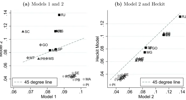
The second column of Table 1 provides returns to schooling estimates using only individuals who work in São Paulo in our baseline sample. For comparison with the previous result, Figure 1a plots estimates of the first two models. Note that the two methods produce very different estimates. For example, Northeastern states’ estimates are the largest in Model 1, but are the smallest in Model 2. Rio de Janeiro (RJ), Espírito Santo (ES), Rio Grande do Sul (RS), and Santa Catarina (SC) also have very divergent estimates. This result is consistent with the idea that skilled labor is scarce in lower income states, so that market forces offer a high reward for education in those regions. Once we use data only on individuals who work in the same labor market, we are able to obtain an improved measure of education quality as valued by market forces.

However, the estimates from Model 2 may still be questionable if we want to interpret returns as educational quality measures. If migrants are positively self-selected, São Paulo’s return to schooling might be underestimated because it is obtained using only non-migrant data. Formally, earnings in São Paulo are obviously not observed for

Table 1: Returns to schooling estimates

Model 1 Model 2 Heckit Model

Maranhão 0.1016 0.0397 0.0328 (0.0007) (0.0044) (0.0042) Piauí 0.1017 0.0311 0.0231 (0.0009) (0.0033) (0.0031) Ceará 0.0932 0.0455 0.0368 (0.0006) (0.0032) (0.0030) Rio Grande do Norte 0.0915 0.0435 0.0376 (0.0008) (0.0058) (0.0057) Paraíba 0.0956 0.0386 0.0310 (0.0008) (0.0035) (0.0034) Pernambuco 0.0895 0.0439 0.0351 (0.0006) (0.0024) (0.0023) Alagoas 0.0938 0.0457 0.0373 (0.0010) (0.0036) (0.0034) Sergipe 0.0951 0.0491 0.0393 (0.0011) (0.0059) (0.0057) Bahia 0.0926 0.0429 0.0335 (0.0004) (0.0016) (0.0016) Minas Gerais 0.0816 0.0834 0.0746 (0.0003) (0.0017) (0.0017) Espírito Santo 0.0848 0.1123 0.1023 (0.0006) (0.0090) (0.0090) Rio de Janeiro 0.0871 0.1371 0.1312 (0.0004) (0.0050) (0.0048) São Paulo 0.0850 0.0850 0.0820 (0.0003) (0.0003) (0.0003) Paraná 0.0749 0.0705 0.0614 (0.0004) (0.0020) (0.0019) Santa Catarina 0.0656 0.1117 0.1026 (0.0004) (0.0085) (0.0084) Rio Grande do Sul 0.0856 0.1125 0.1046 (0.0004) (0.0080) (0.0079) Mato Grosso do Sul 0.0797 0.0709 0.0635 (0.0010) (0.0063) (0.0062)

Mato Grosso 0.0684 0.0720 0.0644

(0.0011) (0.0103) (0.0106)

Goiás 0.0760 0.0916 0.0813

(0.0006) (0.0085) (0.0083) Standard errors in parentheses. All estimates are significant at one percent.

Figure 1: Comparison of educational returns estimates between models

(a) Models 1 and 2

MA PI CE RN PB PE ALBASE MS MT GO PR SC RS MG ES RJ SP .04 .06 .08 .1 .12 .14 Model 2 .06 .07 .08 .09 .1 Model 1 45 degree line

(b) Model 2 and Heckit

MA PI CE RN PBPEAL SE BA MSMT GO PR SCRS MG ES RJ SP .04 .06 .08 .1 .12 Heckit Model .04 .06 .08 .1 .12 .14 Model 2 45 degree line

Geographic regions are identified by different markers: Northeast , Midwest , South , and South-east .

individuals who do not work there. If the decision to work in São Paulo is determined by variables that are correlated to individuals’ years of schooling, estimation of (2) by OLS produces biased and inconsistent estimates. Therefore, we use Heckman’s (1979) selection correction method (the Heckit Model) and postulate that individuals work in São Paulo if

δj+ ηSij + φZij + ψEij + vij > 0, (3) where δj are intercepts that vary across states of birth; Z contains the same variables as X, except for the urban residence dummy; Eij is the (expected) earnings per hour of individual i if she decides to work in São Paulo in relation to working in another state; and v is an error term. Specifically, for an individual working in São Paulo, Eij is equal to her earnings divided by her expected earnings if she were to work in another state. For an individual working in a state other than São Paulo, Eij equals the expected earnings if she was to work in São Paulo divided by her actual current earnings. To calculate expected earnings we use fitted values of linear regressions. That is, we first run a series of regressions of earnings per weekly hours on years of schooling, gender, age, age squared, race, and the urban residence dummy for each possible combination of state of birth and a dummy variable that indicates residence in São Paulo. Then, for example, the expected earnings for working in São Paulo for an individual who studied in Rio de Janeiro is computed as the fitted value of the regression that uses data on individuals who work in São Paulo and were born in Rio de Janeiro. Additionally, we

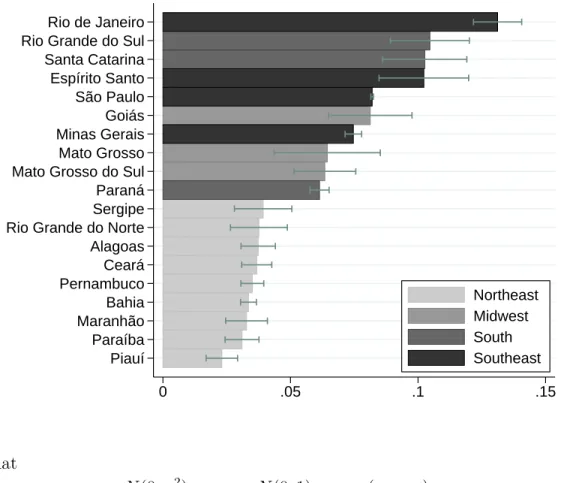
Figure 2: Heckit estimates and 95% confidence intervals Piauí Paraíba Maranhão Bahia Pernambuco Ceará Alagoas Rio Grande do Norte Sergipe Paraná Mato Grosso do Sul Mato Grosso Minas Gerais Goiás São Paulo Espírito Santo Santa Catarina Rio Grande do Sul Rio de Janeiro 0 .05 .1 .15 Northeast Midwest South Southeast posit that uij ∼ N (0, σ2), vij ∼ N (0, 1), corr(uij, vij) = ρ. (4) This is our baseline specification, which we estimate through the Maximum Like-lihood method. For comparison, Figure 1b plots estimates of Model 2 and Heckit. Observe that all states have lower estimates in Heckman’s model, except for São Paulo. This is evidence that migrants are positively selected and that the Heckit model corrects the selection bias by increasing São Paulo’s returns in relation to the other states.

The third column of Table 1 and Figure 2 display returns to schooling estimates that can be interpreted as educational quality measures. Rio de Janeiro and Piauí present the highest and lowest estimates, respectively. That is, after controlling for migration selection issues, if we take two individuals who have studied in Rio de Janeiro, work in São Paulo, and display the same observable characteristics, except for the fact that one individual has one more year of schooling than the other, it is expected that the earnings of the more educated individual are 13.1% higher than the other’s. In contrast, one additional year of education in Piauí, one of the poorest states in Brazil, increases earnings by only 2.3%. The Northeast region unambiguously presents the lowest educational quality, while the other regions display some heterogeneity. Mean educational returns by region are: Northeast 3.4%, Midwest 6.9%, South 8.9%, and

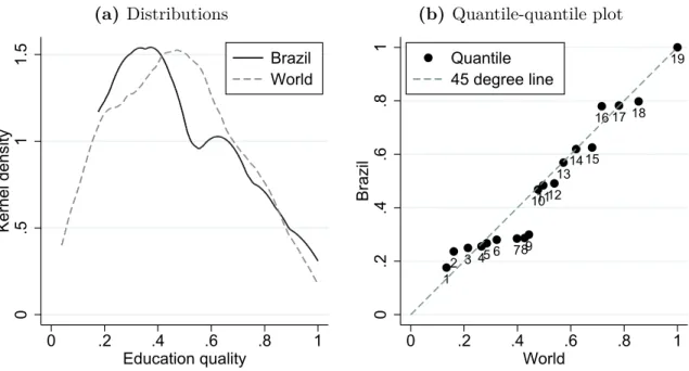
Figure 3: Education quality within Brazil and across countries (a) Distributions 0 .5 1 1.5 Kernel density 0 .2 .4 .6 .8 1 Education quality Brazil World (b) Quantile-quantile plot 1 2 3 45 6 78 9 101112 1314 15 16 17 18 19 0 .2 .4 .6 .8 1 Brazil 0 .2 .4 .6 .8 1 World Quantile 45 degree line

Education quality at country level is given by returns to schooling estimated inSchoellman(2012).

Southeast 9.7%.10

There are important similarities and differences between our education quality index and the education quality measures across countries worldwide produced inSchoellman

(2012). First, education quality in Brazil ranges from 2.3% (Piauí) to 13% (Rio de Janeiro), whereas across the world it ranges from approximately zero (Tonga and Al-bania) to 12% (Switzerland and Tanzania). For reference, Figure 3a plots education quality distributions within Brazil and across countries, after normalizing the largest value of each to one. Instead of arbitrarily selecting numbers in the education quality interval, however, a more appropriate method for comparing the two distributions is to investigate their quantiles. Figure 3bdisplays the quantile-quantile plot for the two distributions. Each dot represents a quantile, out of nineteen, for each distribution. Since we are working with nineteen states in Brazil, each state corresponds to a dif-ferent quantile. The first nine quantiles of the Brazilian distribution correspond to the northeastern states. We can divide the quantiles of both distributions in four subsets: (i) the first three quantiles, (ii) the fourth to the sixth, (iii) the seventh to the ninth, and (iv) the last ten. The dots in the first set lie above the 45 degree line, meaning that the northeastern states with the lowest education qualities have higher relative quality than 10_{Heckman et al.(1996) revisit the literature’s results on the association between education quality} and returns to schooling for the U.S. and find that measured schooling quality only affects the returns for college graduates. We investigate if this is also the case for Brazil by re-estimating our baseline specification, dropping observations for college graduates. The correlation between returns to schooling for the complete sample and this subsample is equal to 0.95. Therefore, our estimates are not driven by the returns for college graduates.

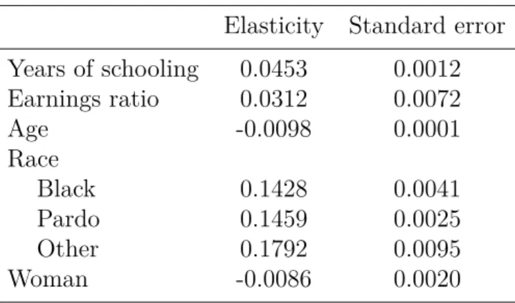
Table 2: Heckit selection equation elasticities

Elasticity Standard error Years of schooling 0.0453 0.0012 Earnings ratio 0.0312 0.0072 Age -0.0098 0.0001 Race Black 0.1428 0.0041 Pardo 0.1459 0.0025 Other 0.1792 0.0095 Woman -0.0086 0.0020

All estimates are significant at one percent. Elasticities in terms of the following variations. Years of schooling and Earnings ratio: one standard deviation increase centered in the mean value. Age: from 35 to 36 years. “Pardo” is a term used by the IBGE that broadly encompasses multiracial Brazilians.

the corresponding countries in the lowest quantiles. The dots in the second set lie close to the 45 degree line, implying that both distributions are similar in this segment. In the third set, the opposite of that observed in set (i) happens. These properties found in sets (i) and (iii) almost perfectly offset each other, so that the Northeast’s mean position in the Brazilian distribution is equivalent to the mean position of countries in the same quantiles in the worldwide distribution. In fact, education quality means in the first nine quantiles of both distributions are not statistically different. In set (iv), the distributions behave very similarly to each other because the dots lie very close to the 45 degree line. Therefore, we conclude that both distributions are quite similar. Consistent with this, the Gini coefficients for both distributions are very close and not statistically different: 0.25 for Brazil and 0.27 across the world.

Table 2shows elasticities related to the coefficients in the selection equation (3). A one standard deviation increase in schooling (expected earnings derived from working in São Paulo in relation to other states) produces a 4.5% (3.2%) higher probability of working in São Paulo. An individual who is 36 years old presents a 0.9% lower probability of working in São Paulo than an individual who is 35.

The correlation between the error terms estimate is ˆρ = 0.7, and the p-value

asso-ciated with the test ρ = 0 is approximately equal to zero. Therefore, we reject the null and conclude that there is selection bias in the estimates from Models 1 and 2.

4

Education quality and other educational variables

In this section we investigate the association between our educational quality measures and standardized test scores, schooling outcomes, and public expenditure on education per schooling stage.

Figure 4: Returns to schooling and Saeb test scores AL BA CE MA PB PE PI RN SE GO MS PR RS SC _MG RJ SP 0 .05 .1 Returns to schooling -2 -1 0 1 2

Saeb test scores (std) beta: 0.025

se: 0.006 p: 0.000 R2: 0.573 corr: 0.757

The solid line and all values in the box, with the exception of “corr,” are related to the OLS estimation between the variables. “corr” denotes correlation coefficient. “std” denotes standardized variable. Ge-ographic regions are identified by different markers: Northeast , Midwest , South , and Southeast

.

adequate comparison in terms of timing, we re-estimate educational returns using the subsample of individuals who were probably studying when the exams were applied, which amounts to selecting individuals between 24 and 32 years of age. Table B5

displays descriptive statistics for this young subsample. Note that there are states for which there is a very small number of migrants in São Paulo, making educational returns’ standard errors very large for those cases. Because of this we exclude states for which there are less than 100 migrants; as a result, Espírito Santo and Mato Grosso are not included in this analysis. TablesB2 and B3 display returns to schooling estimates and selection equation elasticities for this sample. The correlation between the full and young sample educational returns is 0.95.

Figure4displays returns to schooling and standardized Saeb test scores, along with some correlation statistics. The two measures are highly correlated: the correlation coefficient equals 0.75, and a one standard deviation increase in Saeb test scores is associated with an increase in returns to schooling of 2.5 percentage points. However, there are significant differences between both indexes: the Northeast region’s mean Saeb score is equal to 90% of the others regions’ mean. In the case of our educational quality index, this number equals 30%. The Gini coefficients associated with Saeb and our measure are equal to 0.03 and 0.34, respectively. That is, our measure suggests a larger discrepancy between regions’ educational qualities than the Saeb scores do. If we think of our index as the value that market forces assign to education, this is evidence that there are educational components that the market captures, but test scores do not.

Figure 5: Returns to schooling and educational outcomes AL BA CE MA PB PE PI RN SE GO MS PR RS SC MG RJ SP -1 0 1 School attendance (std) -1 0 1 2 Returns to schooling (std) beta: 0.868 se: 0.128 p: 0.000 R2: 0.753 corr: 0.868 AL BA CE MA PB PE PI RN SE GO MS PR RS SC MG RJ SP -1.5 -1 -.5 0 .5 1 Age-grade gap (std) -1 0 1 2 Returns to schooling (std) beta: -0.860 se: 0.132 p: 0.000 R2: 0.740 corr: -0.860

The solid line and all values in the box, with the exception of “corr,” are related to the OLS estimation between the variables. “corr” denotes correlation coefficient. “std” denotes standardized variable. Ge-ographic regions are identified by different markers: Northeast , Midwest , South , and Southeast

.

Next, we investigate the association between our educational quality measures and schooling outcomes at the state level. We use 1991 data on 7- to 14-year-old students’ mean school attendance and 10- to 14-year-old students’ mean age-grade gap by state. To make a compatible comparison, we again use schooling returns estimates obtained using the subsample of young workers. Figure5 displays correlation statistics between education quality and (i) mean school attendance and (ii) the age-grade gap. Note the significant association between the variables: a one standard deviation increase in returns to schooling is associated with a 0.9 standard deviation increase in mean school attendance and a 0.88 standard deviation decrease in the age-grade gap. The high R-squared value also implies that linearity is a good approximation for the relationship between returns to schooling and the educational outcome variables.

The strong association between educational returns and standardized test scores, mean school attendance, and the age-grade gap is evidence that returns to schooling can be used as a proxy variable for educational quality in cases where the latter is not available. Since the use of proxy variables in regressions relies on linearity assump-tions, the evidence for a linear relationship between educational outcome variables and returns to schooling supports this conclusion. For some developing and underdevel-oped countries, educational quality measures are scarce, whereas data on earnings and schooling are readily available. Therefore, verifying the correlation between returns to schooling, test scores, and educational outcomes is relevant for researchers interested in investigating education themes in developing and underdeveloped countries through

the construction of education quality measures.

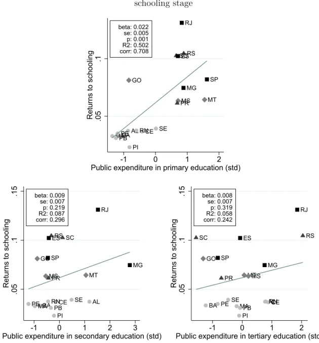
Next, we assess the relationship between educational quality and government ex-penditure on education per student for different schooling stages in 1995. Since the greatest part of students enrolled in primary, secondary, and tertiary education in 1995 were aged 7 to 25, and therefore were 22 to 40 in 2010, we use educational returns estimates obtained using the full sample of workers in 2010. Figure 6 exhibits cor-relation measures between the two variables. First, the association is positive for all schooling stages. However, it is significant only for public investments in primary edu-cation. In fact, the OLS coefficient associated with primary education is greater than the secondary and tertiary education coefficients at 2% and 7% significance levels. The coefficient associated with secondary education is not significantly different from the tertiary education coefficient. This is suggestive evidence that public investments in earlier stages of education are more effective than in later stages, in accordance with the literature discussed in Heckman(2006).

Figure 6: Educational returns and government expenditure on education per schooling stage AL BA CE MA_PBPE PI RN SE GO MT MS PR RS SCES MG RJ SP .05 .1 Returns to schooling -1 0 1 2

Public expenditure in primary education (std) beta: 0.022 se: 0.005 p: 0.001 R2: 0.502 corr: 0.708 AL BA CE MA _PB PE PI RN SE GO MT MS_PR RS SC ES MG RJ SP .05 .1 .15 Returns to schooling -1 0 1 2 3

Public expenditure in secondary education (std) beta: 0.009 se: 0.007 p: 0.219 R2: 0.087 corr: 0.296 AL BA PE MA_PB CE PI RN SE GO MTMS PR RS SC ES MG RJ SP .05 .1 .15 Returns to schooling -1 0 1 2

Public expenditure in tertiary education (std) beta: 0.008

se: 0.007 p: 0.319 R2: 0.058 corr: 0.242

The solid line and all values in the box, with the exception of “corr,” are related to the OLS estimation between the variables. “corr” denotes correlation coefficient. “std” denotes standardized variable. Ge-ographic regions are identified by different markers: Northeast , Midwest , South , and Southeast

5

Development accounting

In this section we conduct a development accounting exercise for Brazilian states. To estimate human capital stocks, we followSchoellman(2012) and parametrize the human capital production function of state j as

h(Sj, Qj) = exp " (SjQj)η η # , (5)

where Sj and Qj denote state j’s mean years of schooling and education quality, re-spectively, and η is an elasticity parameter. We have data on Sj and have produced education quality measures in Section 3. To estimate the production function param-eter, we use Schoellman’s (2012) equilibrium model, which generates a relationship between observable variables that can be used to estimate η.

The equilibrium model features very standard components. Households are com-posed by dynasties. A dynasty is a sequence of workers who are altruistically linked in the sense of Barro (1974). Each worker lives for a finite number of periods, then dies and is replaced by a young worker who inherits his assets but not his human capital. Workers are endowed with one unit of time each period to allocate between school and work. There is a competitive firm that hires labor and rents capital to maximize profits. Education quality is exogenous.

The optimal decisions of workers and firms generate the following equilibrium rela-tionship between quantity of schooling, quality of education, and returns to education,

Mj: log(Sj) = η 1 − ηlog(Qj) − 1 1 − η log(Mj). (6)

In our context, Mj are the returns to education for non-migrants.

Table 3 displays estimates of the elasticity of years of schooling with respect to ed-ucation quality, η/(1 − η), using the specification given by equation (6). The rows also contain the implied value of η and the number of observations used in the regressions. São Paulo is not included in the estimation sample because QSP ≡ MSP. We use two

Table 3: Estimated elasticity of years of schooling with respect to education quality

OLS IV

Unweighted Weighted Unweighted Weighted

Elasticity 0.18 0.25 0.20 0.26

(0.08) (0.07) (0.09) (0.07)

Implied η 0.15 0.20 0.16 0.21

N 17 17 17 17

different estimation methods: constrained OLS and constrained IV. In the latter, we in-strument education quality using 1995 Saeb test scores because returns to education for immigrants may be measured with some error due to small sample sizes (Schoellman,

2012). We find that OLS estimates are close to IV estimates, suggesting that measure-ment error is not a significant issue. We also test a specification where we weight each state observation by the number of immigrants in the sample. In general, the elasticity estimates range between 0.18 and 0.26, which implies that η is between 0.15 and 0.21. These estimates are close to those produced in a robustness exercise in Schoellman

(2012), where ˆη = 0.21. This result is found when one uses Bils and Klenow’s (2000) data on non-migrants’ returns to schooling in order to allow for variability in Mj, in a way similar to our usage here.

Using equations (5) and (6), human capital in equilibrium can be written as log(hj) =

MjSj

η . (7)

This equation is directly comparable to the one used by the development account-ing literature that does not account for quality-adjusted years of schoolaccount-ing (Bils and Klenow,2000), given by

log(hj) = MjSj. (8)

We use equations (7) and (8) to construct quality-adjusted and non–quality-adjusted years of schooling for Brazilian states. Note that the right hand side of these equations differ by a quality markup factor of 1/η, which implies that quality-adjusted log human capital stocks are 4.7-6.6 times larger than non–quality-adjusted stocks.

Since Mincerian returns are noisy, we follow a strategy similar to the one adopted in Bils and Klenow (2000) and Schoellman (2012), and use the trend relationship be-tween schooling and returns to schooling of non-migrants rather than individual state observations in order to compute human capital stocks in (7) and (8). The estimated relationship is

log(Mj) = b1+ b2log(Sj) = −0.68 − 0.80 log(Sj), (9) with standard errors of 0.78 and 0.36.

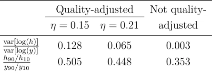
The first two columns of Table 4 display our development accounting results. The first row presents one estimate of the fraction of output per worker differences that is accounted for by quality-adjusted years of schooling, obtained by comparing the variance of log human capital to the variance of log output per worker. Using this metric, human capital accounts for 6%-12% of output per worker differences. According toCaselli(2005), although this measure is nicely grounded in the tradition of variance decomposition, it has the drawback that variances are sensitive to outliers. A measure that is less sensitive to outliers is the inter-percentile differential, obtained by comparing the human capital ratio of the 90th and 10th percentiles to the output per worker ratio of the 90th and 10th percentiles. By this metric, human capital accounts for

44%-Table 4: Development accounting results

Quality-adjusted Not

quality-η = 0.15 η = 0.21 adjusted var[log(h)]

var[log(y)] 0.128 0.065 0.003 h90/h10

y90/y10 0.505 0.448 0.353

50% of output per worker differences. To conservatively summarize our results, we compute the mean between the two measures and conclude that quality-adjusted years of schooling account for about 26%-31% of output per worker differences in Brazil.11

The third column in Table4 shows that using non–quality-adjusted human capital stocks would imply that years of schooling account for about 17.5% of output per worker differences, about 60% of the explanatory power obtained previously. This is evidence that education quality is a very important component to consider if one is interested in studying education in Brazil.

Figueiredo and Nakabashi(2016) construct two quality-adjusted human capital vari-ables for Brazilian states using 2000 data. The first variable relies on Ideb test scores,12 and the second one is based on each state’s mean expected earnings, conditional on the education and experience levels of the working-age population. Our findings are consistent with the results produced through the second variable, which imply that the ratio between the variances of log human capital and output per worker is equal to 0.05, while the inter-percentile differential equals 0.5.13 _{Hanushek et al. (2015) use}

achieve-ment scores adjusted for selective migration to produce human capital stocks for U.S. states, finding that 20%-35% of per-capita GDP variation can be explained by human capital. In terms of cross-country development accounting literature, our results are also quantitatively similar to those found by Schoellman(2012), whose baseline results suggest that quality-adjusted years of schooling account for 21%-26% of output per worker differences.

11_{The findings inHendricks(2002) are similar to ours in the sense that the variance decomposition} and inter-percentile differential measures produce qualitatively distinct results, equal to 0.07 and 0.22, respectively.

12_{Índice de Desenvolvimento da Educação Básica (Ideb) is an educational quality index developed} by Inep, and embodies Saeb test scores and approval rates. We do not consider Ideb in this paper because it is available only from 2005, a relatively recent year. Our dataset contains information on individuals who were working in 2010, and most of them studied many years before 2005.

13_{Figueiredo and Nakabashi’s (2016) human capital variable produced through Ideb test scores} displays very large variability, generating variance and percentile ratios equal to 0.37 and 0.72.

6

Conclusion

In this paper we provide a new measure of education quality for Brazilian states in 2010, based on the idea that the financial returns obtained from an additional year of schooling can be seen as being derived from the value that the market assigns to this education. We use census data on migrants in the state of São Paulo in order to estimate returns to schooling of individuals who obtained education in different states, but who work in the same labor market.

We find that educational quality is very heterogeneous across states, following the large economic inequality in Brazil. In fact, our index implies that education quality is more unequal across states than standardized test scores imply. This is a relevant result for the debate on educational quality in Brazil, suggesting that there are educa-tional aspects that market forces capture, but standardized test scores do not. Further research is warranted in order to disentangle which elements each method considers.

We document a strong correlation between our education quality measures and stan-dardized test scores and educational outcome variables, supporting the use of returns to education as an educational quality index.

We find that higher educational quality is significantly associated with greater public expenditure on primary education at the state level, but insignificantly related to higher public expenditure on secondary or tertiary education. This is suggestive evidence that public investments in earlier stages of education are more effective than in later stages, in accordance with the literature discussed inHeckman(2006). However, the Brazilian government’s expenditure per student in tertiary education in 2008 was equal to 1.17 of OECD countries’ mean expenditures. For the case of secondary and primary education, these proportions were equal to 0.22 and 0.30 (OECD,2011). Our results reinforce the pool of stylized facts that motivate rethinking the Brazilian government’s education investment profile.

Finally, we conduct education quality-adjusted development accounting exercises for Brazilian states and conclude that human capital plays an important role in explaining output per worker differences. Ignoring education quality reduces human capital’s ex-planatory power by 40%, suggesting that this is an important component to consider if one is interested in understanding economic development within regions of a country.

References

J. Abrahão and M. A. C. Fernandes. Sistema de informações sobre os gastos públicos da Área de educação – SIGPE: Diagnóstico para 1995. Texto para Discussão 674, IPEA, 1999.

A. Banerjee and E. Duflo. Poor Economics: A Radical Rethinking of the Way to Fight

R. J. Barro. Are government bonds net wealth? Journal of Political Economy, 82(6): 1095–1117, 1974.

M. Bils and P. J. Klenow. Does schooling cause growth? American Economic Review, 90(5):1160–1183, 2000.

B. Bratsberg and D. Terrell. School quality and returs to education of U.S. immigrants.

Economic Inquiry, 40(2):177–198, 2002. ISSN 1465-7295. doi: 10.1093/ei/40.2.177.

URL http://dx.doi.org/10.1093/ei/40.2.177.

D. Card and A. Krueger. Does school quality matter? Returns to education and the characteristics of public schools in the United States. Journal of Political

Econ-omy, 100(1):1–40, 1992. URLhttp://EconPapers.repec.org/RePEc:ucp:jpolec: v:100:y:1992:i:1:p:1-40.

F. Caselli. Accounting for cross-country income differences. Handbook of Economic

Growth, 1:679–741, 2005.

B. Chiswick and P. Miller. The effects of school quality in the origin on the payoff to schooling for immigrants. IZA Discussion Papers 5075, Institute for the Study of Labor (IZA), 2010. URL http://EconPapers.repec.org/RePEc:iza:izadps: dp5075.

P. Ferreira and C. Santos. Migração e distribuição regional de renda no Brasil. Pesquisa

e Planejamento Econômico, 37(3), 2007.

L. Figueiredo and L. Nakabashi. The relative importance of total factor productivity and factors of production in income per worker: Evidence from the Brazilian states.

EconomiA, 17(2):159–175, 2016.

E. Hanushek and L. Wobmann. Education Quality and Economic Growth. The World Bank, 2007.

E. Hanushek, J. Ruhose, and L. Woessmann. Human capital quality and aggregate income differences: Development accounting for U.S. states. Working Paper 21295, National Bureau of Economic Research, June 2015. URL http://www.nber.org/ papers/w21295.

J. Heckman. Sample selection bias as a specification error. Econometrica, 47(1):153– 162, 1979.

J. Heckman. Skill formation and the economics of investing in disadvantaged children.

J. Heckman, A. Layne-Farrar, and P. Todd. Human capital pricing equations with an application to estimating the effect of schooling quality on earnings. The Review of

Economics and Statistics, 78(4):562–610, 1996.

L. Hendricks. How important is human capital for development? Evidence from immi-grant earnings. The American Economic Review, 92(1):198–219, 2002.

IPEADATA, 2016. URLhttp://www.ipeadata.gov.br/.

A. Krueger and M. Lindahl. Education for growth: Why and for whom? Working Paper 7591, National Bureau of Economic Research, March 2000. URL http:// www.nber.org/papers/w7591.

Q. Li and A. Sweetman. The quality of immigrant source country educational out-comes: Do they matter in the receiving country? CReAM Discussion Paper Series 1332, Centre for Research and Analysis of Migration (CReAM), Department of Eco-nomics, University College London, Dec 2013. URL https://ideas.repec.org/p/ crm/wpaper/1332.html.

OECD. Education at a glance 2011: OECD indicators, 2011. URLhttp://www.oecd. org/edu/school/educationataglance2011oecdindicators.htm.

T. Schoellman. Education quality and development accounting. The Review of

Eco-nomic Studies, 79(1):388–417, 2012.

A. Sen. Development as Freedom. Anchor, 2000.

B. Sianesi and J. van Reenen. The returns to education: Macroeconomics. Journal of

Economic Surveys, 17(2):157–200, 2003. ISSN 1467-6419. doi: 10.1111/1467-6419.

Appendix

A

Categorical schooling variable

In Section3 we used imputed schooling data because the 2010 census does not provide the exact number of individuals’ years of schooling. An alternative to this imputation is using a categorical schooling variable that identifies the following years of schooling intervals: from 0 to 3 years, 4–7, 8–10, 11–14, and 15 years or more. We proceed in two steps. First we estimate Heckman’s model, modifying equation (2) to

log(Wij) = αj + 5 X

k=1

βjkDijk+ γXij + uij, (10)

where k assumes the 5 possible values of the categorical schooling variable and Dijk is a dummy that indicates if individual i’s schooling belongs to interval k. We also use the categorical schooling variable in the selection equation (3). This step produces 4 schooling coefficients for each state (one of them is omitted to avoid collinearity). Second, we compute for each state the weighted mean of schooling coefficients using the fraction of individuals in each schooling interval as weights. The result is an average of marginal effects for each state.

FigureA1plots Heckman’s model estimates using imputed and categorical schooling variables. Both methods produce qualitatively similar results. Note that averages of marginal effects have different magnitudes than the educational returns estimated previously. This happens because those estimates no longer have the interpretation of an expected increase in earnings due to one additional year of schooling.

FigureA2 and Table A1 display returns estimates. Confidence intervals are signifi-cantly larger in this case because we estimate 160 additional parameters. Besides this, standard errors increase when we compute the weighted average of marginal effects.

Figure A1: Returns to schooling estimates (imputed and categorical schooling variable) MA PI CE RN PB PEAL SE BA MS MT GO PR SC RS MG ES RJ SP .3 .4 .5 .6

Heckit Model (Categorical Variable)

.02 .05 .08 .11 .14

Heckit Model (Imputed Variable) corr: 0.968

Geographic regions are identified by different markers: Northeast , Midwest , South , and Southeast .

Figure A2: Heckit estimates and 95% confidence intervals (categorical schooling

variable) Maranhão Piauí Paraíba Bahia Ceará Pernambuco Alagoas Rio Grande do Norte Sergipe Mato Grosso Mato Grosso do Sul Paraná Minas Gerais Goiás São Paulo Espírito Santo Rio Grande do Sul Santa Catarina Rio de Janeiro .2 .4 .6 .8 Northeast Midwest South Southeast

Table A1: Returns to schooling estimates (categorical schooling variable)

Estimate Standard error

Maranhão 0.2486 0.0369***

Piauí 0.2676 0.0307***

Ceará 0.3172 0.0251***

Rio Grande do Norte 0.3567 0.0564***

Paraíba 0.2950 0.0299*** Pernambuco 0.3382 0.0198*** Alagoas 0.3488 0.0310*** Sergipe 0.3642 0.0479*** Bahia 0.3019 0.0138*** Minas Gerais 0.4719 0.0143*** Espírito Santo 0.5247 0.1013*** Rio de Janeiro 0.6539 0.0680*** São Paulo 0.5192 0.0032*** Paraná 0.4544 0.0169*** Santa Catarina 0.5965 0.1065***

Rio Grande do Sul 0.5319 0.1027*** Mato Grosso do Sul 0.4026 0.0624***

Mato Grosso 0.3889 0.1259**

Goiás 0.4948 0.0711***

N 5,478,685

B

Other tables

Table B2: Returns to schooling estimates (young sample)

Estimate Standard error

Maranhão 0.0141 0.0067**

Piauí 0.0191 0.0061**

Ceará 0.0379 0.0082***

Rio Grande do Norte 0.0330 0.0175*

Paraíba 0.0273 0.0087** Pernambuco 0.0330 0.0067*** Alagoas 0.0272 0.0085** Sergipe 0.0253 0.0095** Bahia 0.0194 0.0033*** Minas Gerais 0.0836 0.0046*** Rio de Janeiro 0.1186 0.0224*** São Paulo 0.0683 0.0005*** Paraná 0.0782 0.0069*** Santa Catarina 0.0862 0.0172***

Rio Grande do Sul 0.1230 0.0333*** Mato Grosso do Sul 0.0515 0.0127***

Goiás 0.0855 0.0212***

N 1,671,545

* p < 0.10, ** p < 0.05, *** p < 0.01.

Table B3: Heckit selection equation elasticities (young sample)

Elasticity Standard error Years of schooling 0.0422 0.0028*** Earnings ratio 0.0520 0.0057*** Age 0.0799 0.0362** Race Black 0.1480 0.0076*** Pardo 0.1449 0.0047*** Other 0.1474 0.0177*** Woman 0.0046 0.0038

* p < 0.10, ** p < 0.05, *** p < 0.01. Elasticities in terms of the following variations. Years of schooling and Earnings ratio: one standard deviation increase centered in the mean value. Age: from 24 to 25 years. “Pardo” is a term used by the IBGE that broadly encompasses multiracial Brazilians.

Table B4: Descriptive statistics (means) and number of observations by state of birth and residence

Years of schooling Earnings per weekly hours Number of observations

Living in Living in Living in Living in Living in SP Living in other states

State of birth SP other states SP other states N Percent N Percent

North 9.97 8.90 56.50 36.41 900 0.08 302,443 6.37 Rondônia (RO) 8.81 9.18 39.09 38.56 76 0.01 21,079 0.44 Acre (AC) 11.69 9.00 71.92 40.88 26 0.00 15,145 0.32 Amazonas (AM) 11.71 9.25 83.12 40.46 107 0.01 57,536 1.21 Roraima (RR) 10.06 10.25 40.98 46.67 10 0.00 5,849 0.12 Pará (PA) 9.95 8.55 58.08 33.85 538 0.05 144,028 3.04 Amapá (AP) 8.40 10.28 48.24 44.67 27 0.00 11,669 0.25 Tocantins (TO) 8.73 9.00 25.16 32.53 116 0.01 47,137 0.99 Northeast 6.40 8.32 31.84 31.10 46,975 4.43 1,450,167 30.56 Maranhão (MA) 7.38 8.31 33.40 31.05 2,359 0.22 172,019 3.63 Piauí (PI) 6.48 8.14 28.78 30.54 3,327 0.31 100,120 2.11 Ceará (CE) 6.49 8.41 32.73 30.58 5,068 0.48 210,466 4.44

Rio Grande do Norte (RN) 6.87 8.60 35.81 31.93 1,209 0.11 99,191 2.09

Paraíba (PB) 6.09 7.95 30.48 31.21 3,632 0.34 130,828 2.76 Pernambuco (PE) 6.25 8.53 35.59 32.37 8,956 0.85 220,999 4.66 Alagoas (AL) 6.05 7.94 28.81 30.18 3,813 0.36 72,298 1.52 Sergipe (SE) 6.61 8.14 31.33 31.23 1,413 0.13 58,106 1.22 Bahia (BA) 6.40 8.31 30.60 30.73 17,198 1.62 386,140 8.14 Southeast 10.33 9.29 55.16 43.02 995,079 93.90 1,359,010 28.64 Minas Gerais (MG) 7.61 8.63 46.87 36.79 16,989 1.60 794,327 16.74

Espírito Santo (ES) 9.09 8.86 52.77 38.11 460 0.04 121,494 2.56

Rio de Janeiro (RJ) 11.59 10.13 107.44 50.06 2,682 0.25 356,863 7.52

São Paulo (SP) 10.37 10.25 55.14 58.44 974,948 92.00 86,326 1.82

South 8.08 9.05 48.27 40.05 14,349 1.35 1,288,899 27.16

Paraná (PR) 7.48 9.00 39.28 39.05 12,387 1.17 439,176 9.26

Santa Catarina (SC) 10.52 9.00 84.40 40.21 757 0.07 296,395 6.25

Rio Grande do Sul (RS) 11.37 9.13 97.88 40.84 1,205 0.11 553,328 11.66

Midwest 9.17 9.35 51.32 44.71 2,384 0.22 344,428 7.26

Mato Grosso do Sul (MS) 9.09 9.01 46.07 38.06 1,062 0.10 67,681 1.43

Mato Grosso (MT) 8.18 9.20 36.83 38.94 471 0.04 60,399 1.27

Goiás (GO) 9.23 9.05 57.77 42.19 714 0.07 193,879 4.09

Table B5: Descriptive statistics (means) and number of observations by state of birth and residence (young sample)

Years of schooling Earnings per weekly hours Number of observations

Living in Living in Living in Living in Living in SP Living in other states

State of birth SP other states SP other states N Percent N Percent

Rondônia 10.23 9.47 30.12 30.88 21 0.01 12,833 0.84 Acre 12.21 9.84 24.49 31.15 5 0.00 5,836 0.38 Amazonas 13.16 9.93 64.23 33.05 19 0.01 21,609 1.41 Roraima 10.98 37.22 0 0.00 2,565 0.17 Pará 11.15 9.18 54.87 26.28 97 0.03 57,581 3.77 Amapá 8.39 10.84 70.17 31.95 2 0.00 4,614 0.30 Tocantins 8.55 9.86 22.46 26.03 38 0.01 18,569 1.22 Maranhão 7.42 9.12 25.74 24.91 761 0.22 63,344 4.15 Piauí 7.19 9.14 25.10 24.13 876 0.25 32,798 2.15 Ceará 7.82 9.66 35.67 23.72 806 0.23 69,830 4.57

Rio Grande do Norte 9.45 9.64 40.51 23.90 119 0.03 32,730 2.14

Paraíba 6.71 8.97 27.77 23.76 554 0.16 40,566 2.66 Pernambuco 7.64 9.39 34.54 25.71 1,281 0.37 73,779 4.83 Alagoas 6.69 8.61 26.85 22.98 780 0.23 25,116 1.64 Sergipe 8.14 9.13 24.23 24.50 214 0.06 19,785 1.30 Bahia 7.86 9.34 25.68 24.13 3,262 0.95 136,785 8.96 Minas Gerais 10.04 10.08 46.35 28.87 2,133 0.62 237,876 15.58 Espírito Santo 12.87 10.22 58.43 30.49 62 0.02 38,488 2.52 Rio de Janeiro 12.72 10.89 86.50 38.71 348 0.10 109,662 7.18 São Paulo 11.34 11.26 41.59 40.05 331,496 96.19 26,155 1.71 Paraná 10.20 10.36 46.30 32.12 1,056 0.31 137,158 8.98 Santa Catarina 12.27 10.59 80.49 33.30 137 0.04 90,006 5.89

Rio Grande do Sul 13.05 10.54 92.94 32.32 170 0.05 147,332 9.65

Mato Grosso do Sul 10.54 9.95 41.82 30.95 180 0.05 24,949 1.63

Mato Grosso 10.53 9.95 30.18 30.90 74 0.02 26,784 1.75

Goiás 11.45 10.31 62.39 35.73 115 0.03 59,386 3.89

Distrito Federal 12.83 11.68 77.92 57.17 37 0.01 11,097 0.73

Total 11.23 9.99 41.43 30.06 344,643 100 1,527,233 100