STEEL MECHANICAL PROPERTIES EVALUATED AT ROOM TEMPERATURE AFTER BEING SUBMITTED AT FIRE CONDITIONS

Eds.: Oktay Ural, Vitor Abrantes, António Tadeu

STEEL MECHANICAL PROPERTIES EVALUATED AT

ROOM TEMPERATURE AFTER BEING SUBMITTED AT

FIRE CONDITIONS

Piloto, P.A.G1; Vila Real, Paulo2; Mesquita, Luís3; Vaz, M.A.P.4

1,3

Applied Mechanics department, Polytechnic Institute of Bragança, Ap. 1134, 5301-857 Bragança, Portugal e-mails: ppiloto@ipb.pt; lmesquita@ipb.pt

2

Civil department, University of Aveiro, Campus Santiago, 3810 Aveiro e-mail: pvreal@civil.ua.pt

4

Mechanical department, Engineering Faculty - University of Porto, Rua Dr. Roberto Frias S/N e-mail: gmavaz@fe.up.pt

Key words: mechanical properties, fire conditions, residual stress relief, metallurgic phase transformation

Abstract

1 Introduction

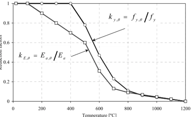
For steel structures under high temperature the relationship between stress and strain changes considerably. At high temperature, the material properties degrade and it’s capacity to deform increases, which is measured by the reduction of the Young’s modulus [1]. Basic material research of structural steel materials is becoming more important as the significance of fire engineering design of steel structures is growing and new steel materials, including high-strength steels and stainless steels are going to be used more widely in steel structures in the near future [2,3].

The load bearing capacity after fire conditions mainly depends on the fire duration, critical temperature and on the cooling process phase. The structural material behaviour will be very important, regarding its mechanical properties after being subjected to metallurgic transformations. During fire conditions, the structural material will be charged with high thermal gradients at elevated temperatures that may produce metallurgic transformations, according to the steel equilibrium diagram represented in figure 1. In general, very slow cooling rates from elevated temperatures will follow the iron – iron carbide equilibrium diagram. Any rate of cooling, interpreted as nonequilibrium, should be analysed by using the time – temperature – transformation (TTT) curves [4], as represented in the figure 2.

Figure 1: Iron – iron carbide equilibrium diagram [13].

Figure 2: Continuous cooling transformation curve [4].

Lines of different slopes on this diagram can show the effect of the cooling rate. Slow cooling may lead to the formation of pearlite ferrite mixture. Cooling at an intermediate rate passes through pearlite/ferrite transformation at higher temperatures, but changes to bainite transformation at lower temperatures so that a mixture of pearlite and bainite results. A higher rate in the cooling phase may result in phase transformation to martensite after passing through the two horizontal lines. Thus in practice, varying the cooling rate may produce different steel composition and resultant properties [8]. The material under testing is a steel S275 JR with 0.16% carbide, 1.15% Mn, 0.24% Si, 0.008% P, 0.01% S, 0.05% Cr, 0.05% Ni, 0.01% Mo, among other chemical elements, as reported in the inspection certificate from the manufacturer.

2 Steel mechanical properties at elevated temperatures

2% to represent the yield of the material have been established. The results of Rubert and Schaumann [10] were transposed to the Eurocodes, and they have established a model in which the material creep would be considered in a implicit way.

In the linear elastic range, the Elastic Modulus will change due to the increasing of temperature as can be seen in the figure 3, representing this material property with a reduction coefficient.

0 0.2 0.4 0.6 0.8 1

0 200 400 600 800 1000 1200

Temperature [ºC]

Reduction factors

a a

E E E

k _,θ = _,θ

y y

y f f

k _,θ = _,θ

Figure 3: Reduction coefficient for yield strength and for elastic modulus.

This variation is the result of a tabulated relationship between the value of the Elasticity Modulus at elevated temperature and the reference value at room temperature (equation in figure 3) [11].

After several experimental and numerical campaigns, Franssen [12] propose analytical expressions to represent the behavior of yield strength. In Eurocode 3 [11], this mechanical property variation is presented in tabulated data, with a coefficient that references the material property value at high temperature to the value at room temperature (equation in figure 3) [11].

3 Experimental

procedure

Several specimens were submitted to high different temperature conditions and to different cooling rates (natural cooling and quenching). The mechanical properties have been compared regarding the material strength, HRB and HRC hardness and its metallurgic microstructure. The heating phase was achieved using the electro ceramic mat resistance (see figures 4 and 5), at constant rate equal to 800 [ºC/hour]. The temperature was controlled at two different points and the cooling phase controlled by another thermocouple.

Figure 4: Beam thermocouple instrumentation.

Figure 5: Beam heated at 800 [ºC] during one hour.

Figure 6: Beam cooling procedure (quenching).

distinct phases. First, the water in contact with the piece heats rapidly to its boiling point and converts to steam, forming a film or blanket around the metal and insulates it form the liquid water. As the metal cools, the violent generation of steam subsides and some of the liquid becomes in contact with metal surface, even with boiling going on, promoting a high heat transfer rate. When enough heat is removed, the steel losses the ability to convert the liquid into steam and the liquid cooling stage begins [15].

4 Tensile

tests

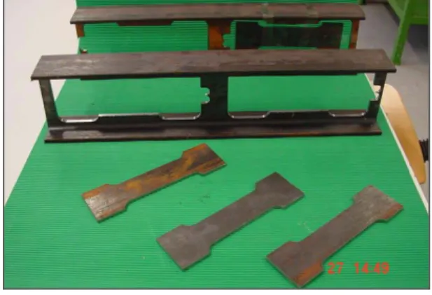
The process for determining the yield stress has been carried out as closely to code [7]. The specimen has been machined from the web of the steel beam element, has shown in figure 7, according to the dimensions of each specimen.

0.00E+00 1.00E+08 2.00E+08 3.00E+08 4.00E+08 5.00E+08 6.00E+08 7.00E+08 8.00E+08 9.00E+08 1.00E+09

0.00 0.05 0.10 0.15 0.20 0.25 0.30

Strain [mm/mm]

Stress [Pa

]

P05 - temp.=500 [ºC] - quenching after 1hour P04 - room temperature P06 - temp.=800 [ºC] - quenching after 1hour

P18- temp.=600 [ºC] - natural cooling after 1hour

Figure 7: Samples location and specimens geometry.

Figure 8: Stress – Strain curve for specimens tested at different conditions.

The speed increment for each part of the stress strain curve has been used according the standard [7]. The specimens were tested on a universal testing 4885 Instron machine with the data acquisition system GPIB assisted by a personal computer. The resultants stress – strain curve are shown in the figure 8, regarding four different material conditions. The yield range has been specially analyzed to present the results in table 1. represents the ultimate stress while and represents the higher and lower yield stress.

m

R ReH ReL

Table 1: Tensile test results at room temperature.

Test

R

_eH[MPa]

R

_eL[MPa]

R

_m[MPa]

R

_p0.2[MPa]

A

_t[%]

P01 492 499 575 492 34.5

P02 511 493 592 507 33.5

P03 507 498 580 505 35.0

P04 525 508 597 518 28.9

Average ± Sdv 509± 14 500± 6 586± 10 506± 11 33.0± 2.8

In the case of brittle material, the yield stress should be considered equal to ₂ and the extension

after collapse _t will be smaller. Several specimens were heated during 1 hour at each different temperature level followed by quenching. The results are presented in table 2.

. 0 p

R

Table 2: Tensile test results after being submitted to high temperatures and quenching.

Test Temperature [ºC]

R

_m[MPa]

R

_p0.2[MPa]

A

_t[%]

P05 500 498 391 20.60

P08 500 532 453 25.30

P13 500 552 469 40.00

P16 500 576 493 37.00

P12 600 575 500 24.35

P14 600 506 429 31.00

P15 600 512 382 30.00

P09 700 506 294 22.12

P06 800 974 687 1.74

P07 800 988 717 7.10

P11 800 987 786 9.67

P10 850 1140 758 9.76

Other testing conditions were carried out with the same steel material and with natural cooling rate. The results are presented in the table 3 according to the typical stress strain curves with residual stress relief. The tested specimens P18 and P19 presents yield strength level that is 100 [MPa] smaller than the normal state condition.

Table 3: Results from the tensile tests at several temperatures with natural cooling.

Test Temperature [ºC]

R

_m[MPa]

R

_p0.2[MPa]

A

_t[%]

P17 500 515 482 36.98

P20 500 580 501 36.76

P18 600 485 410 29.61

P19 600 474 390 36.86

The test P17 and P20 could not achieve the transition temperature for stress relieving, producing a standard stress-strain curve.

5 Hardness

tests

The hardness Rockell B and C was measured over the entire cross section from the top flange till the bottom, passing through the web. The precision in this measuring is in compliance with ISO 716 standard and the method according to ISO 6508 and Portuguese standard NP4072 [5]. The penetrator used for measuring Rockwell B was a ball with 1/16´´ diameter, with a preload of 10 [kgf] and a load of 100 [kgf], while for measuring Rockwell C, 120º diamond penetrator was used with the same preload and 150 [kgf] of total force. The time suggested to load and unload the specimen was 6 [s]. The average results of 39 measured points over the entire cross section from the IPE specimens were made for several different conditions, according to the next table.

Table 4: Rocwell B and C hardness results from specimens at different conditions.

Test Temperature [ºC]

Dwell Time [hour]

Water cooling Hardness HRBm Average ± Sdv

Hardness HRC Average ± Sdv

1 20 - - 92.9 ± 1.4 -

2 600 1 yes 85.0 ± 3.2 -

3 600 1 no 81.6 ± 3.3 -

4 800 1 yes - 38.6 ± 2.4

5 850 1 yes - 40.3 ± 4.2

6 Metallography

analysis

The metallurgic analysis was made at several different state conditions. At room temperature the specimens were cutted from two different zones. Those two specimens were transversally cutted from the IPE 100 cross section and both surface were prepared in three different phases (pre polishing, polishing and chemical attack). In the first phase the specimen must be prepared without scratches and spots. The polishing phased is normally executed by fine abrasives and should produce a specular bright and undeformed microstructure. The chemical attack (nitric acid 5 [cm3] plus 100 [cm3] of ethylic alcohol) should be used during 30 seconds maximum, in order to obtain a good optical contrast regarding different metal elements, different phases and different orientation in grain size. This procedure was made with reference [6] and in accordance to ASTM E 3-62 and ASTM E 7-63.

At room temperature is possible to see the two-equilibrium phases material (ferrite and pearlite), as expected and represented in the figure 9.

200 x – web 200 x - flange 1000 x - web 1000 x - flange

Figure 9: Microstructure from steel in received conditions from the manufacturer.

For the case of a steel heated at 800 [ºC] during one hour and with a rapid cooling the microstructure expected will be martensite or eventually bainite, as can be inspected from the figure 10.

200 x – web 200 x - flange 1000 x - web 1000 x - flange

Figure 10: Microstructure from steel after 1 hour at 800 [ºC] and quenching cooling.

7 Residual stress relief

The magnitude and geometric distribution of the residual stresses may vary with the geometry of the cross section and with the straightening and cooling processes. The idealized distribution is expressed in the figure 11 and will be used to measure the residual stress in a specific point of the beam length.

Figure 11: Residual stress – theoretical distribution and origin [13].

intersection zone from web and flange will shrink after the other zones and some plastic flow will be induced.

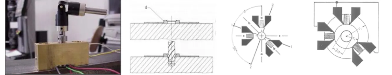
The hole drill method covers the procedure for determining residual stresses near the surface of isotropic linearly-elastic materials [14]. The use of special strain gauges will be necessary and a mechanical interference will be introduced into the specimen. The requirement of keeping the disturbance as small as possible is a positive factor in this method. The drill hole rosette shown in the figure 12 requires a small drill hole of about 1.5 [mm]. This can be regarded as a non-destructive technique [9] or as a “semi-destructive” because the damage that it causes is very localized and in many cases does not affect the usefulness of the specimen [14].

Figure 12: Residual stress measuring set-up with strain gauges rosette from HBM RY61.

The residual stresses were measured before and after the material being submitted to high temperature conditions. The objective of this experiment was to see if the stresses were relieved with the used temperature level. The residual initial stresses could be determined by the measured deformations

a

ε

∆

,

∆

ε

_b and

∆

ε

_c and by the elasticity theory, determined from the center of the flange, point of maximum residual stress value. In this experimental procedure a type A rosette [14] was used with the following dimensional geometric characteristics: a=0.75[mm], ri =1.8[mm], ra =3.3[mm].

The principal directions “1” and “2” may be calculated with the simple formula (2), based on the measured strains, using a two-argument arctan funtion.

      ∆ − ∆ ∆ − ∆ + ∆ = a c b c a arctg ε ε ε ε ε ϕ 2 2

1

(

)

(

) (

2

)

2

2 ,

1 2

4

4 a c B a c b c a

E A

E _{ε ε ε ε ε ε ε}

σ =− ∆ +∆ ± ∆ +∆ − ∆ + ∆ −∆ (2)

The results shown that the principal directions were align with the tested profile, as expected. The stresses may be computed form equation (2), considering that a tensile residual stress will produce negative relived strain and A and may be calculated according to the geometric properties of this strain gauge and material properties [9]. The results before and after stress relief are presented in table 5, demonstrating that this type of methodology may reduce the internal and initial residual stresses in structural elements.

B

Table 5: Measured residual stresses and principal directions.

Specimen [ºC]

Temperature [ºC] /

Dwell time [h] / Heat rate [ºC/h]

σ

1 [MPa]

σ

2 [MPa]

ϕ

=

σ

C [MPa]

Test 1 No 165,0 96,7 100 162.9

Test 2 No 191,0 121,0 109 183.6

Test 3 600 / 1 / 800 95,8 78,4 147 89,9

The stress represents the tension state in the flange along the profile direction. As represented in figure 11, a symmetric value should be expected in the web that should be responsible for the same amount of difference between tensile tests P18-P19 (see table 3) and P01-P04 (see table 1).

C

σ

8 Conclusions

process that may happen after accidental situation. If the material temperature exceeds the transition to austenithique phase a brittle material may be achieved, depending on the cooling process. In case of natural cooling the material will relief its residual stress ∆σ_C in the some amount as the difference between the strength tensile tests, depending on the temperature level induced (550-650 [ºC]). The hardness tests were done for all different studied cases, expecting higher results for brittle material. Two different scales were needed. The metalographic analysis is in accordance to the measured results.

The amount of stress relief is in agreement with the difference result of the tensile tests.

Acknowledgments

This work was performed in the course of the research project PRAXIS/P/ECM/14176/1998, sponsored by the Portuguese Foundation for Science and Technology. Special thanks are due to the enterprise J. Soares Correia.

References

[1] Sanad, Moniem Abdel; Behaviour of steel framed structures under fire condition – British steel fire test1; research report R99-MD1; University of Edimburgh; December 1999.

[2] Outinen, Jyri; Kaitila, Olli; Mäkeläinen; High-temperature testing of structural steel and modeling of structures at fire temperatures - Research report; Helsinki University of Technology laboratory of steel structures publications - TKK-TER-23; Espoo 2001.

[3] Outinen, Jyri; Kesti, Jyrki; Mäkeläinen; Fire Design Model for Structural Steel S355 Based Upon Transient State Tensile test results; Journal Construct Steel Res.; Vol. 42, No.3, pp 161-169; 1997.

[4] Pollack, Herman W.; Materials Science and Metallurgy; 4th edition, Prentice Hall – A reston book, 1988, USA.

[5] CT12 – Instituto Português da Qualidade; Norma Portuguesa NP 4072 – Materiais metálicos – Ensaio de dureza. Ensaio Rockwell (escalas HRBm e HR30Tm); Outubro 1990.

[6] LNEC – Laboratório Nacional de Engenharia Civil; Norma Portuguesa NP1467 – Aços e Ferros Fundidos – Preparação de provetes para metalografia; Port. Nº 321/77; Junho de 1977.

[7] CT12 – Instituto Português da Qualidade; Norma Portuguesa NP EN 10002-1 – Materiais metálicos – Ensaio de tracção. Parte 1: Método de ensaio (à temperatura ambiente); Novembro 1990.

[8] Owens, Graham W.; knowles, Peter R.; Steel Designers Manual; The Steel Construction Institute; 5th edition; Blackwell Scientific Publications, GB, 1992.

[9] Hoffman Karl; An introduction to measurements using strain gages; HBM publisher; Germany; 1989. [10] Rubert A.; Schumann P.; Temperaturabhangige Werkstoffeigenshaften von baustahl bei

Brandbeanspruchug; Stahlbau; Verlag Wilh. Ernst & Sohn; Berlin; 54; Heft 3; 81-86; 1985.

[11] ECS ENV 1993-1-2; Eurocode 3 – Design of steel structures – Part 1-2: General rules – Stuctural fire design; 1995.

[12] Franssen, J.M.; Etude du comportment au feu des strutures mixtes acier béton, Thèse de doctorat; Collection de la F.S.A. ; Nº111; Univ. de Liège, Belgium.

[13] ESDEP Society; European Steel Design Education Programme; UK; CD-Rom version; 1999.

[14] ASTM – Committee E28.13; Standard Test Method for determining Residual Stresses by the Hole Drilling Strain Gage Method; E837-01; USA; January 2002.