/.
4.
..
,.
"
"
"
'-'
~ ~"
...
"
"
"
...
-.
"
...
"
...
-.
...
...
"
-.
"
...
...
...
...
-.
...
"
"
•
..,
.. ..
~ \...\..
..
CAIXA POSTAL 9.052 - CEP 22253
RIO DE .JANEIRO· R.J - BRASIL
C I R C U L A R
N
26 2
Assun~o: Seminário de Pesquisa Econômi ca I I C 1 51 par ~e)
Coordenadores: Fernando de Holanda Barbosa
Convidamos V. Sa. para par~icipar do Seminário/EPGE a ser·
realizado na pr6xima 551 feira:
DATA:
22/1 0/Q2•
HORARIO:
15: 30hLOCAL:
Audi ~6r i o Eugêni o Gudi nTEMA:
"URBAN EARNINGS INEQUALITY IN BRAZIL AND ARlJEWl'I NA:COHPARATIVE ANALYSIS··. pelo Prof. Lauro R. A. Ramos CIPEA:> .
. /MARF
de Janeiro. 20 de ou~ubro de 1992.
M G. DE ANDRADE ia-Geral/EPGE
BB-00064631--6 ~ ~ ~ .,j ~
.
. j . j ~""
.,
~"'"
"'"
. j ~ . j"'"
"'"
"'"
-.J
. j-.J
."ttJ .ti . j ~ ~ .ti-.J
.ti .ti .ti ~-.J
.."..,
..,
'fII 'fII•
•
•
•
.,
..
.,
.I
.I
.,
.,
'"
•
...
...
...
"
-.
..
....
....
"
"
"
...
...
...
...
...
...
...
..
...
...
...
"
...
"
...
"
...
...
"
...
...
"
"
...
..
~, ~URBAN INCOME INEQUALITI IN ARGENTUU AND BRAZIL: A COMPARATIVE ANALYSIS
Alber~ Fishlow
*
Ariel Fiszbein**
La.uro Ramos ***INTRODUCTION
1. VARLATIONS IN THE INCOME DISTRIBUTION 2. DECOMPOSITION ANALYSIS
3. RETURNS TO EDUCATION
A. Est~ating Income Differentials
B. Explaining the Different Patterns in Returns to Education C. Testing Alternative Hypotheses
4. CONCLUSIONS Tables and Figures Appendix 1
Appendix 2 Appendix 3 References
(*) University of California, BerkeleYi (**) The World Bank; (***) IPEA; the views expressed here are those of the authors and should not be at~ributed to the institutions they belong.
- - - - -~ ~ ~ ~ ~
-
~--
•
---•
•
•
•
---
-•
-•
---
•
---
-
~ ~ ~•
~ ~ ~----
-URBAN INCOME lNEQUALITY IN ARGENTINA AND BRAZIL:
A COMPARATlVE ANALYSIS
INTRODUCTION
Albert Fishlcw Ariel Fiszbein Lauro Ramos
The decade of the 1980's for the Latin American countries nas been one of unprecedented decline even in comparison with the 1930's. Not surprisingly, the consequence has been a concentration upon macroeconomic issues at the expense of others. But the high degree of inequality found in Latin America snould remain amatter of serious concern, the more so since the supposed negative relationship between macroeconomic performance and the income distribution undergirds much of the opposition to orthodox stabilization policy.
In this essaywe examine the comparative response of the size distributions in Argentina and Brazil to economic deterioration in the beginning of the 1980's. Such a methodology takes advantage of the available annual income distribution data, and also allows comparison of the responses in an economywnose performance was already stagnating, Argentina, with one whose growth rate had been the highest and steadiest in the region, Brazil. This distinction turns out to be a central part of the explanation we offer to the ratner áifferent results tnat emerge in each of the countries.
In Section I, we present a summary of changes in the distributions in the
two countries over more than the last decade. In Section 11, we decompose the
observed changes in inequality into two component parts, the economic structure
of the labor force and relative earnings. In Section 111, because i t is changing
relative incomes with respect to education that account for the largest part of the changes in inequality, we examine the time pattern of returns to different leveIs of education in the two countries. Our explanation for the distinct
cyclical variation of returns in Brazil and its absence in Argentina turns on different processes of labor carket aàjustment in the countries.
1. VARIATIONS IN TRE INCOME DISTRIBUTION
Tables 1 and 2 present infor::Ilation on the income distributions in Argentina and Brazil from tne mid-1970's to tne 1980's. wnile tne Argentine data refer to tne Buenos Aires metropolitan area and the Brazil information is for males in
urban areas only,l other information confirms that they are representative.2 The time pattern of the Argentine urban labor force as a yhole is sicilar, and the -. exclusion of female yorkers in Brazil does not alter the observed cycle, or
-.
-.
"
-
-.
..,
...
..,
..,
"
-.
...
-.
..,
..,
..,
..,
..,
-.
'-'.
leveIs of inequality.JTwo principal conclusions emerge from tnese tables. One is the much higher inequality in Brazil than Argentina, regardless of measure. í..is distinction carries through even more vividly were the measurement to limit itself to the percentage of the population in poverty. Thus, yhile the percentage of the Brazilian population in poverty yas 17.7 in 1980 and 23.3 in 1987 (Fox and Morley [1990]), the incidence of poverty in the case of Argentina yas only 8% in 1980 and 13% in 1987 (CEPAL [1985] and (1989b]). Higher Argentine income per capita and a lesser dependency ratio accentuate the divergence in measures of inequality. Even in 1981 yhen the difference betyeen the CYO countries is at its 1The Argentine data are from the Buenos Aires Household Survey ("Encuesta Permanente de Hogares") undertaken by the Argentine National Institute of Statistics and Census (INDEC). The Brazilian data are from the "Pesquisas Nacionais
t
Amostra de Domicilios" (PNADs) and correspond exclusively to males in urban a eas. A more complete description of the data is provided in Appendix1. ~ .
lSee Bonelli and Sedlacek (1991] and Barros and Reis (1990].
~easures of inequality yere calculated for a set of ten urban areas in Argentina for 1974, 1980, 1982, and 1985. The Gini coefficients yere 0.36, 0.42, 0.41, and 0.42 respectively. For the consequences of excluding female yorkers in the Brazilian case see Ramos (1990].
..
--
.--
-.
-.
--
-.
-.
-.
-.
-.
-.
...
..
-.
...
...
...
...
...
...
-.
...
...
...
...
-.
minimum, t~e bottom 60 percent or the Argentine distribution receive almost 30 percent of the income while the comparable Brazilian group accounts ror less than 24 percen~. This difference is grea~er than ~~e entire earnings or the bottom quintile.
Of special concern here, however, are the divergen~ time trenàs in the ~~o
countries. In Argentina, there is a clear increase cver time in the degree cr inequality, as ~he Gini coefficient rises from .34 in 1974 to .45 in 1988. This increase is very subs~antial relative to deteriorations recorded in cther countries. A simple experiment reveals its magnitude.' If in 1974 a lump-sum tax equal to 21.6% of the Argentina per capita income had been levied on alI individuaIs earning below the median -equal to almost t-..1ice as great a percentage of that group' s income- and redistributed t::l those above the median, the equivalent 1988 inequality would have resulted. A significant rise occurs between 1976 and 1978, anà again between 1985 and 1988 .
For Brazil, the results exnibit no trend, but rather a cyclical variation over the period. Inequality declines from 1976 through 1981 and then rises steadily almost to replicate its initial value in 1985. As Figures 1 and 2 graphically reveal, there is an inverse conformity to income per capita in this variation. As income growth continued at the end of the 1970's inequality began to decline, and as income per capita actually fell frem its 1980 peak, ... deterioration of the distribution likewise occurreà. Recovery after 1983 was . . associated with resumed improvement in a Theil measure or inequality in 1984, but -. not with the Gini coefficient.
Note that the Brazilian pattern of changing inequality rejects a dominant role for wage policy berween 1979 and 1983 as an important leveler. During that interval, indexation was integral for groups earning up to three times the minimum wage, but only partial for higher wages. In principIe, such a disparity would have produced greater equality. It is clear from these data that other
sources of relative income changes dominated this policy effect.
'See Blackburn (1989] for a methodological description or the experimento 3
-.
...
...
...
...
...
-.
~-..
...
...
...
...
...
...
...
...
...
...
...
...
...
...
...
...
...
...
...
...
...
...
...
...
...
...
...
...
...
~-The Argentine ineome per eapita series is marked by its t=enâ decline over this period. But this does not translate into a eomparable negative assoeiation
~ith inequality, despite the eonsisteney of the aggregate direeticn of change . From 1978 to 1983, inequality is relatively stationary ~hile tne income decline is at its greatest; and the sharp decline in 1985 corresponds to tne brie: inc~e
spurt associated ~ith the initial success of tne Austral Plano
This difference in the patterns in the two countries provides us ~ith our - basie question: ~hy? \oIhat processes ~ere at ~ork to produee such a large increase in inequality in Argentina ~hile in Brazil there ~as evidence of improvement during the first part of the period followed by later decline? Note, moreover, that later data for Brazil, extending to 1989 show a ne~ pattern of decline, associated ~ith rene~ed income stagnation, after 1986.5
2. DECOMPOSITION ANALYSIS
An
important step towards a better understanding of the socio-economic mechanisms responsible for the changes in the ineome distribution is the decomposition analysis. This technique allows one to separate t" ... o principal sourees of variation in measured inequality, income and allocation changes. For the class of additively decomposable inequality measures, as shown by Shorrocks(1980), i t is possible to break down the change in inequality becweent~o points of time aecording to ~hether it ean be attributed to modifieations in the socioeconomic groups relative incomes, relative group sizes or in their internal inequalities .
The inequality indices of this elass can be ~itten as:
'"
...
..
...
...
...
... yhere a, ~s the ratio betyeen the average income of ggroup g and tne average
..
...
...
...
...
...
...
...
...
-.
..
.. ..
..
...
..
..
..
..
...
..
.. ..
.. ..
...
..
...
...
..
...
~-income of the yhole population, 3, is the propor~ion oi the population in grcup
g, and I, is the internaI dispersion of incomes in group g. In this context, the
composition or allocation effectS corresponds to the variation induced in the
inequali':y index I by modifications in the allocation of the population among the groups (changes in the 3s), Yith no direct changes in the group relative incomes (as).7 The income effect corresponds to the changes in I induced by changes in group incomes (as), yithout changing the group population shares (35), and the internaI effect is the change in the inequality caused only by modifications in the dispersions at group level (the 1,s).
Therefore, in order to allCY a Kuznetian characterization of the changes in the income distribution,' tne composition effect snould be of considerable magnitude and more important than the income effect. wnen the reverse takes place, i.e, yhen the income effect outplays the allocational changes, then tne reasons for the alterations in the distribution should be related to the suplly and demand for the particular profiles under study. Finally, if neither of them happen to be of considerable significance, one can say that the explanation for the changes in inequality is not related to that particular stratification of the population .
Tnere are three indices, among the most commonly used, that belong to this class: the coefficient of variation and the first and second Theil's measures of
'The difference betyeen this and yhat Knight and Sabot (1983) call the
"compression" effect is that in the present exercise ye are including the indirect change induced in I through the variation in the yeights of the l,s •
70 f course the individuals as change as the Bs change, since the overall
average income is altered. Nevertheless, given that the relative group average incomes remain the same, this indirect impact is aIs o computed in the composition effects (see Appendix 2).
'The Kuznets inverted U-curve of inequality as income rises yas attributed by him to the shift from lcy income rural activity to higher income urban industry and services. In an initial phase, the increased heterogeneity of the labor force yould lead to increase in measured inequality, yhile in the second phase, there yould be increased homogeneity as more and more of the labor force moved to tne seconoary ano tertiary sectors.
...
.. ..
.-.,
.. ..
.,
..
..,
..,
..
..
...
..,
..
..
....
....
..
....
..,
..,
,.,
..
..
....
..,
....
....
..
..
..
..,
....
..,
..
inequality - the Theil T anã Theil L, respectively. In this essay we nave cnos·en to use a decomposition of th.e Theil T:i th.e coeificier.t of variation was discardeã for not satisfying the principle
oi
composite transfers established by Shorrocks and Foster (1985)10, and the preference over the Theil L was ~ainly due to its its wider use in the literature .The ciecomposition was performed according to the following expressicn, whose analytical derivation is shown in Appenci~ 2 •
G G G
dT=
L
aJln(Xg+Tg-T-l)dPg
+L
PJln(Xg+Tg-1)
d(Xg
+L
tIgPg
(l)g-l g-l g-l
Then the gross ccntribution of a variable can be defined as the sue of the income anã allocation effects corresponding to the decomposition accorciing ~c
that variable taken alone. On the other hand, the marginal contribution of a variable is the additional contribution to the explanation of the variations in
inequality when that variable is added to a model already containing other variables .
We àecompose inequality changes here into the following potential explanatory personal characteristics: education, position in occupation, and sector, in the case of Argentina, and the same three variables with the addition of age in the case of Brazil.l l These are the principal available variables that in other studies have successfully captured the variation in individual income levels, and here too explain much of the variance •
'Most of the times in the text we will reier to i t simply as Theil indexo 10See Ramos (1990].
llThe number of variables that could be used in the decomposition in the case of Argentina was limited due to the relatively smaller number of observations. The choice of the variables was done on the basis of the importance of their gross contributions. See Appendix 1 for a description of categories used in tne àecomposition.
-.
~..,
..
..,
..
..,
..,
..
..,
..
..,
..
..,
..,
..,
...
..
.. ..
..,
..,
..,
..
...
..,
..
..
..,
...
...
...
..,
..,
..
~..
..
~-\olhen applied to observed changes in inequality in the tTJo countries, a very similar result cbtains. For ali cnaracteristics and periods, tne variations in the distribution turn out to be dcminated by relative income effects. In the case
of Argentina, tvo-thirds or the observed rise i~ inequality derive rrem
differential earnings!2; in the case or Brazil, a narro,.,ing oi relatiV'e i~comes
explains almost half of t~e improvement from 1977 to 1981, and just above half
of the deterioration in 1981-85. Indeed, in the case or Brazil, not only is the composition efrect close to zero, but actually negati'le: in a Kuznets f r ame,.,ork, cne ,.,as beyond the turning point .
Secondly, i t is the variation in the returns to education in both countries
tnat is more related to measured changes in inequali~y, particularly in tne case
or Argentina ,.,here i t alone explains more than halr of tne measured changes . Sector of activity turns out to be much less important, reflecting the relatiV'e stability or tne observed intersectoral ,.,age differentials .
The variable position i~ occupation is important in tne Brazilian case,
rivalring ,.,ith education in both subperiods, but not for Argentina, where its gross and marginal contributions are small and negative in the second subperiod, despite somewhat high values in the first. This variable differentiates betTJeen employers, employees, and those ,.,ho are self-employed. It may be regarded as a partial proxy for wealth and family status, capturing both changes in tne functional distribution and additional elements not represented by education . Thus, in tne case of Brazil, its behavior can be related to a process of capital deepening at the end of the 1970s, which came to an end in the beginning of tne 1980s during tne period structural aàjustment tnat greatly squeezed real wages •
For Argentina, its relative i~portance in the 1974/80 period may be asociated to
the deterioration in the functional distribution of income that took place as a consequence cf tne institutional transfor:nations resulting frem the 1976 military coup (Orsatti (1983]).
12This is consistent with the findings of CEPAL' s (1986) study cf the
cnanges in tne aistributien betveen 1974 anà 1983.
3. RETURNS TO EDUCATION
The ciecomposition analysis has shown the central role playeà by cnanging relative incomes Yith respect to eàucation, in accounting ror t~e cnanges in income inequaIity. Thus, ye ncrw turn our attention ~o educational cifferentials and examine the time pattern of returns to àifferent leveIs of eciucation in t~e
tYO countries.
Tables 5 and 6 shcrw t:-"e principal parameters determining ~:-"e cnanges in the distribution by leveI of educa~ion. IndividuaIs have been categorized in similar '" groups in the 1:'".10 countries. The group Yith elementary eàucation in Brazil
'"
....
....
...
...
..
....
-.
....
..
....
...
.,
.,
..
...
...
....
....
.,
~ ~ ~ ~ ~-.
-.
....
...
..
..
includes individuaIs Yith one to four years of schooling, and thus corresponds to the group Yith less than pr~ary education in Argen~ina.:3 The percentage of illiterates in the Argentine case yas negIigible .
Even thougn both countries present signs of educational expansion (for example, the percentage of individuais Yith university eàucation doubled in Argentina and increased by almost 50% in Brazil), the allocation effect yas not
important in explaining the changes in inequality .
In the case of Argentina we find an upyard trend in educational income differentials. For example, yhile in 1974, on average, individuais yith university education earned 2.9 times the income of individuaIs yith less ~han
primary education, in 1980 they earned 3.4 times, and in 1988 3.9 times. In the case of Brazil, table 6 shcrws some evidence of a cyclical behavior of differentials. For example, individuaIs Yith university eciuca~ion earneci 8.2 times the income of illiterates in 1977, 7.3 times in 1981, and 7.9 times in
1985 •
Ramos (1990) used three synthetic measures to summarize the changes reIated to education: mt
, that represents the average leveI of schooling of the labor
lJThose yho have completed their primary education have at Ieast seven years of schooling.
•
•
•
•
•
•
•
•
•
•
•
•
•
•
force, I.
..
-
,
which corresponds to the degree of inequality in the distributionof education, I~ ano s , that sw::cari:::es the variations in the inccme ratios • t
associated with education.:s
The results for Brazil and Argentina are shown in Table 7. r.~e figures in
there just confirm the steady improvements in the mean leveI of education in both
countries, adding up to an increase of 14: in Argentina in a span of 14 years,
and to tne same 14% in Brazil in a span of 8 years (~e cannot compare tne
• absolute leveis of the index ~ for the CWo countries, as they are on differente
. . 'scales"). What is very surprising is that the inequality of education
• deteriorates in alI periods for Argentina, and in the first one in the case of
• Brazil. 17 This findind highlights the fact that an i::lprovement of the
•
•
•
..
..,
..,
•
...
..
..
..
...
...
...
...
...
...
...
-.
~. ~ ~ ~ ~ ~ ~..
-.
~ ~educational levei does not necessarily translate into a better distribution of schooling, at least up to a point (the Kuznets' turning point, as a matter of
fact). I : also helps to explain tne nature of the composition ettect: al~ays
positive in the case of Argentina, ~hereas small and even negative for Brazil .
The behavior or the income profiles related to education, as indicated by st, also points to a continuous deterioration in Argentina and a U-pattern in
14 t m l:1 a 113"1' '" • where a 1 represents t e '" h standardized income of the
educational category i in the base year. For Brazil the year chosen as the basis was 1981 and, accordingly, we have: a*1 - 0.137, a·% - 0.217, a-J ... 0.273, a*. ,.
0.423 and a'"~ - 1.0. For Argentina the basis year is 1980, leading to: a-I ,.
0.137, a· z - 0.217, a'"J - 0.273, a*. - 1.0 •
1~it ,. (l/mt) .l:1a *ta \10g(a*1) - log(mt) , that corresponds to the Theil T index
that would prevail in a population with no inequality within the educational groups, and where the group incomes were proportional to the group average incomes in the basis year.
Ust ,. (1/l:1a\a'"1) l:1a \a*110g(a\) - 10g(l:1a \a*1)' -which can be understood as an
indicatcr of the relative steepness of the income profiles related to education. If one fixes the the fraction of the labor force in each educational group, i t follOYs that the steeper the income profile the larger the bet-ween group
inequality (as before, the as -were also fixed for 1980 and 1981).
17In spite of this continuous deterioration, education is still much better
distributed in Argentina than in Brazil. 9
.,
.,
...
...
...
...
..
..
.,
..
..
..
Brazil. Given that the income distribution displayed this very same evolution, the income effects associated to schooling are, accordingly, alyays positive.:s In both ccuntries the cnanges yere mucn more pronounced in s~ tnan in i:, ynat lends additional support to a more cautious investigation or t~e evolution of the scnooling income differentials .
. , A. Estimating Income Differentials .
..
.,
.,
.,
.,
.,
..,
..,
..,
..,
.,
..,
..,
..,
..,
..,
..,
This evidence on relative incomes for different educational classes confirms patterns first found in overall income inequality: a trend toyard higher inequality in Argentina, and cycli=al behavior in the case of Brazil. In order to explore these different patterns ye have estimated income differentials associated Yith education, controlling for a number of additional variables .
A concise Yay of estimating the returns to scnooling is by using conventional earnings equations based on the human capital paradigm, Yith controls for other characteristics that might influence the differentials. 19
This approach alleys one to disentangle the association beween individual earnings and leveIs of education frem the joint influence of other variables on earnings. It can be summarized by the relation Y - f (S,Z), dY/dS > O, yhere Y represents labor income, S is the number of years of schooling, and Z is a set of control variables •
.., There are three points tnat one needs to pay attention to in order to .., estimate the earnings differentials associated to scnooling in this frameyorK .
...
..,
18It 1s yorth noticing that steeper income profiles, higher inequality in
the distribution of education, and the overall explanatory poyer of education are the key factors to understand yhy the income distribution is much vorse in Brazil than in Argentina.
l~e are deliberately ignoring alI the debate about the pertinence of this paradigma, as this discussion is not vithin the scope of the paper. It should be stressed, hovever, that despite alI the disagreement on the specific role education plays in the formation of earnings, no scholl of tnought denies its major importance in tnat processo
-.
.. ..
-.
-.
-
- First, we have to consider the question of causality. We are :'r.terested in--
..
"
-"
"
-"
-.
"
...
"
"
--"
"
..
"
"
"
..
-.
.. ..
-.
..
..
.. ..
-.
~-.
-.
~-.
measuring the change in an individual's earnings if sne, and only sne, wnere to increase her education from, say, the leveI s to s+l. This differential cannot be directly measured, as i t envolves the difference between an observed variable (the wage sne actually gets) and an unobserved one (the wage she would receive if she were more educated). The usual way cut is to assume tnat the wage she would obtain unàer these circumstances is just the average wage of individuaIs that in fact are in the s+l educational leveI, and are otherwise identical to her (i.e., display the sace set of characteristics depicteà by Z). Therefore, under this assumption, the observed differentials would correspond to the actual
changes induced by marginal improvements in educaticn.20
Of course the aàequacy of this assumpticn depenas on tne "homogeneity" of the groups formeà by the set of variables Z. The second point relevant for the
estimation aÍ returns to eàuca~ion, nence, concerns che choice oÍ Z. According
to the human capital theory, some of the variables in Z should be experience, ability, and family backgrounà, among others. Unfortunately these variables are not easily observable, and there is no consensus that they exhaust the set of income determinants. Therefore, the design of Z is somewhat arbitrary in the literature. The contraI variables used in this essay, for both countries, were age, sector of activity, and position in occupation. Additionaly, we used gender,
in the case of Argentina, and geographic region, in the case of Brazil.21
Finally, there is also t'~ the question of the most adequate
functional form for f(S,Z). There is a wide range aÍ possibilities here, most of them of an ad hoc nature. Again, we followed this tendency and cpted for the following specification:
20See Barros and Ramos (1991] for a formal discussion oÍ this issue.
21The Argentine data did not allow the use of geographical regions. The size of the Brazilian data set permitted us to concentrated the analysis on males only, therefore avoiding the question of gender differences in the labor market attachmenc.
.. ..
..
..
..
..
..
.. ..
..
..
where:vector of individual earnings in year t;
a: logaritb~ of the mean income of t~e reference group i~ year t;
b~~t : wage cif:erential associated to the itn group of variable ; for year t;
x .
matrix of explanatory variables (S,Z) for year t;vector of residual terms ror year t, E(utl -
°
anã E(utu:'] - a:I •Tables 8 anã 9 present the estimates of the differentials associated with . . education for Argentina anã Brazil respectively. The coefficients in the . . regression are converted to indices. The reference group is individuaIs with less . . than primary educatio~ in the case of Argentina and i~dividuals with elementary . .
..
education i~ the case of Brazil.22.. ..
..
..
..
...
..
...
...
...
The results in table 8 snow tnat, i~ Argentina, i~come differentials for individuaIs with high-school and university education followed an upward trend during this period. Their income differentials increased frem 1974 to 1980, were relatively stable becween 1980 and 1985, and increased again from 1985 to 1988 .
In contrast to those for better educated individuaIs, income differentials for individuaIs with primary education did not follow any clear pattern throughout
h ' . d 23
t ~s per~o •
In the case of Brazil individuaIs with intermediate, high-scnool and ... university education experienced decreases in their income differentials prior 21 The nature of the two data sets, and the characteristics of the educational composition of the labor force in the ~~o countries, did not allow adopting exactly the same specification. However, as indicated above, these two groups are roughly similar.
21.1hen the null hypothesis 1374-13so-13s$-/3u (where 13 is t1:e coefficient multiplying the variable education in the earnings equation) was tested for individuaIs with university and high-school education, the p-values were lower than 0.1%. The p-value i~ tne case of individuaIs with primary education was
to 1981, and increases since tr.en. Income differentials for the group óf
..
illiterates followed a somewhat erratic pattern.'
..
-. As we had anticipated frem the decomposition analysis, in ooth countries-. the patterns of change in returns te different leveIs
oi
educatior.al achievement -. appeared to mimic those in overall income inequality, as measured in tables 1 and -. 2. In the case of Argentina the two periods in which the inccme inequality -. increased significantly were periods in which returns to education also -. experienced significant increases. In the case of Brazil, the same cyclical~ variation found in income inequality is seen in returns to education.
-.
..
..
...
-.
"
-.
...
...
...
..
"--.
-.
-.
-.
-.
...
...
...
'-'
B. Explaining the Different Patter~s in Returns to Education .
The Brazilian data reviewed so far, suggests that ec.ucational inccme differentials (and inccme inequality) vary counter-cyclically. One pertinent hypothesis is related to the effects of short run fluctuations in the leveI of output and real income on the operation of labor markets. The literature on labor "hoarding,,2' suggests that wage differentials between skilled and non-skilled labor tend to increase during economic slumps, and to narrow in the upper part of the business cycle. Accordingly, the distribution of earnings within the active labor force would exhibit a cyclical behavior, improving during periods of excess demand and worsening in times of excess supply.
When labor is regarded as not a fully variable factor of production but as
quasi-fL~ed (meaning that part of its total empIoyment costs are fixed as a resuIt of hiring and training costs), the amount of labor input to be used is no longer determined exclusively on the basis of the current relation betweenwages 2'iffien the null hypothesis (137."13,0·135,'"'13ss ) was tested for individuaIs with
university and high-school education, the p-values were lower than 0.1%, while for individuaIs with intermediate education i t was 1.5%. The p-value in the case of illiterates was 24%.
VSee Oi (1962), Okun (1981], Coleman [1984J, and Fay and ~edoff [:985J,
among others.
..
..,
..,
..,
..,
..,
..,
..,
...
...
...
...
...
...
...
•
...
..,
...
...
...
...
...
-.,
-.,
•
...
..,
..,
~and marginal value product, but also cn t::e basis cf their expected future values. In the short run, the hir~ng anà training costs are perceived as sunk costs. Thus, labor demand and vages for factors vith relatively high degrees of fixity become less cyclical than thcse for factors vith l~ àegrees cf f~~ity . More quali:ied vorkers (better educated vorkers) tend to embcdy higher leveIs of training costs. Accordingly, cne cf the main predictions of tne labor hoarding hypothesis i5 that vage distributions viII display a cyclical behavior, vith differentials shrinking during booms and expanding during recessions .
In tne case of Brazil, the economic slovdovn tnat started in tne early 1980' s came after a period of strong and sustained grovth. Expectations vere that the economy vould go through a brief period cf adjustment after vhich grOYth vould resume. Thus, consistently vith the labcr hoaràing hypothesis, it vas less skilled (less educated) vorkers that experienced most of the adj ustment in employment and vages, leading to increased income aifferentials and i:lccoe inequality .
In contrast to Brazil, vhich in this period experienced traditional business cycles, Argentina experienced an almost constant decline in econcmic activity during period under analysis. The economic slovdovn associatea vith the debt crisis and the international recession cf the early 1980's came atter a period of stagnation rather t:::.:'l cne of sustained grovth. In such an environment labor hoarding, as a response to short run and temporary fluctuations in output no longer is an attractive alternative to firms.26
In an environment of economic stagnation/decline, insti~utional factors 5eem to play a more important role in influencing income differentials than in the context of a groving economy. Faced vith changes in aggregate demand vhich do not seem to be of a transitory nature, as vell as vith uncertain future inflation rates, firms tend to regard the official vage policy as the main (and probably best) signal indicating the future evolution of vages. As a result, Z'The saroe reasoning should apply for the rest of eighties in Brazil, as the economic slump ceased to be perceived as snort :asting. See Ramos and Trindade
-.
-.
-.
....
..
..
--..,
.. ..
..
policies of -wage restraint, exemplified by reductions in the real value of"Salarios Basicos", 27 are generally emulated by emplcyers in the private sector,
particularl: in the case of blue-collar, produc~ion -workers •
-. The absence of economic dynamism, like the one found i~ Braz~l t~rcugnout
" the 1970's, further expanced the lac~ of competition in t~e labor market i~ the
-. Argentine case. The Argen~ine state became a central player in the distri~utive
. . conflict as the -wage policies i t follO'Wed became an important source of:hange
-. in the size distribution of income.
-.
..
-
-.
..
..
...
...
...
...
...
.. ..
..
....
..
...
...
..
..
.. ..
~-..
~ ~ ~-.
..
...
...
...
~c.
Testing Alternative Hv~otheses.We -will use the non-parametric "sign" test in order to assess t~e
explanatory po-wer of the ~~o hypotheses discussed above.Z8 The existence of a
cyclical relationship bet-ween income differentials and economic performance in the short run-will be assessed testing the null hypothesis that differentials are independent of a measure of the business cycle, against the alternative that there is a negative association bet'Ween them. The existence of a relationship bet'Ween income differentials and the direction of the official -wage policy -will be assessed testing the null hypothesis that differentials are independent o: changes in the minimum -wage/basic -wage •
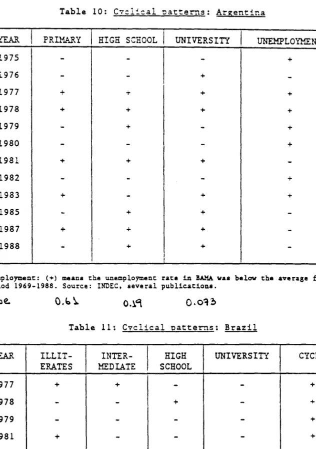
Tables 10 and 11, evaluate the existence of a counter-cyclical behavior in income differentials. For the case of Brazil a measure of potential income -was used. In the Argentina case no such a measure -was available, and thus -we used the unemployment rate, a reasonably accurate measure of activity, instead •
21The "salarios basicos de convenio" are supposed to be determined by collective bargaining, for different occupations by industry. In fact, during most of the period under consideration there -was no collective bargaining, and
thus basic -wages -were adjusted on a regular basis by the govemment.
ZIThese tests relate the direction (the "sign") of the changes in income
differentials, rather than their =agnit~des, to the sign of a ~easure of the
state of the business cycle and to the direction of the changes in minimum'Wages. 15
ti.
~ ~-.
.. ..
'"
..
...
-.
..
-.
-.
-.
-.
..,
...
..,
-.
...,
...,
...
-.
..
...
...
...
...
...
..
...
...
...
-.
...
...
..
-..
'-~...
...
-..
~...
-.
...
..,
..
The hypothesis of cyclical differentials performs very ~ell for Brazil. For individuals ~ith high-school anci university eciucation, the sign or the cyclical component of output ~as different from the sign or the variation i~ t:'e differential in seven out of eight years. Accordingly, the associated p-va :~e fer the test is 0.035, meaning that the null hypoehesis of independence becween shor-: run economic performance and the relative income of ~orkers ~ith higher leveIs of education can be rejected in favor of the hypothesis stressing a c~unter
cyclical pattern. The null hypothesis cannot be rejected in the C:lse of ±ndividuals ~ith intermediate schooling (p-vaIue 0.145) as ~ell as in t:'a case of illiterates (p-value 0.965). This conforms to expectations, given an association of skill and educational leveI.
The hypothesis of counter-cyclical income differentiaIs does not perfor.n
~ell in the case of Argentina. The p-values corresponding to the null hypothesis of no relationship bet~een the cycle and income differentials ~ere 0.073 for individuaIs ~:.,:h university education, O .1938 for those ~ith coeplete high-school, and 0.613 for those ~ith primary education. The nuIl hypothesis of independence cannot be rejected .
Tables 12 and 13 evaluate the existence of a negative relationship between the direction of the official ~age policy and the change in returns to educatio~ . This hypothesis performs very ~ell for Argentina. For individuaIs ~ith hig school and university education, the sign of the change in basic ~ages ~·a.s
different from the sign of the variation in the differential in ten and eleven out of t~eIve years respectiveIy. Accordingly, the associated p-values for the teses are 0.003 and 0.019. The null hypothesis or independence bet~een t:'e direction of the official ~age policy and the relative income of ~orkers ~it~
higher leveIs of education can be easily rejected. The same relationship is not found in the case of individuals ~ith primary education, for ~hom the p-value i5 0.194. This should not be a surprise given that the changes in that group's income differentials ~ere found to be insignificant.29
nSee footnote 12.
..
"
"
.~"
-.
-.
.. ..
~..
~"
-.
~-.
..,
..,
.. ..
-.
...
.. ..
..,
-.
-.
..,
..
.,
..,
..
"
..,
..
"
"
-.
'-'
~ ~The same hypothesis was tested for Brazil with negative results. The null
hypothesis that there is no reIationsnip between cnanges i~ the minimum wage and
returns to education cannot be rejected. The p-vaIues are 0.637 for individuaIs with high-scnool and university education, 0.363 for those with intermeàiate
scnooling, anà 0.856 for iIIiterates.
The evidence just reviewed confirms our previous finding that returns to eàucation nave behaved differentIy in the two countries. Inccme differentials "J.ssociateá with education appear to mo .... e counter-cyclically in Brazil, wnile no clear presence of such a pattern could be found for Argentina. The same evidence suggests that official wage policies in Argentina may have had an important effect on àifferentials, whiIe no similar pattern is present in the Brazilian data.
4. CONCLUSIONS .
In this essay we have examined the changes that have taken place in the size distribution of income in Argentina and Brazil since the mid 1970's. The economic performance of the two countries, throughout the periods we analyzed, have been of a quite different nature. In the beginning of the 1980's, when the international debt crisis started, Argentina was already going through a process of economic stagnation while Brazil was the country where the growtn rate had been the highest and steadiest in the region.
Our researcn has shown chat tne changes that took pIace in the BraziIia~
size distribution of income, most notably the reduction in returns to education
~'C\-i.~\I"f
until 1981 and their posterior increase, were associated with the fIuctuations in the leveIs of economic activity. Thus, income inequality fell during the period of growth, and later increased as a result of the economic slowdown of the early 1980's.
-. In the case of Argentina, we have found that the 1980's show evidence of
~ a continuous deterioration in the size distribution of income which started in
17
..
~"
...
...
...
...
...
"
"
"
"
"
"
...
...
"
...
"
...
"
"
"
...
"
"
...
...
...
"
...
"
"
"
"
"
-.
-.
~ ~ ~'-'
...
....
...
"
-.
...
..,
the 1970's, before the beginning of the international debt crisis. Our
interpreta~ion of the increased leveIs of i:lequali~y in the Argentine case focuses on the role playea by official .... age policies in the ccntext of an economy that is experiencing an almost continuous process of decli~~.
We have founa evidence to support the assertion that, 1:1 the Brazilian case, the macroeconomic shocks of the early 1980's and the policies they induced, .... ere an important factor explaining the reversal of the improvements i:1 the size
distribution of income that took place in the secona half of the 1970's. The deterioration in the Argentine size distribution precedes the macroeconomic crisis of the 1980's, although the latter probably deepenea the original trend in income inequality .
This comparative analysis highlights the importance of studies .... nich carefully assess the links bet'óo1een the economic decline of tne 1980' s anci increased i:lcome inequality in other Latin American countries. It also indicates tnat both market forces and policy variables must be consiaered in any explanation.
~ ~
'-'
--..
~"
-"
'-'
"
'-'
'-'
"
..
"
"
"
"
.. ..
"
"
"
..
"
-
"
-
-.,
-
.. ..
-..
..
--
~ ~ ~ ~ ~ ~--.,
...
"
-TABLES ANO FIGURES
Table 1:
B~.A: Distribution Al1l0ng Economical17 Act:"le POtlula!:i.cn
Bottom
Middle
Middle
Top GiniTheil
Theil
20% 40%
High
10%Dec .
30% 1974 6.8 29.0 37.4 26.8 0.344 0.221 0.190 1975 6.3 29.4 37.9 26.4 0.347 0.212 0.193 1976 7.0 27.9 37.9 27.2 0.352 0.211 0.199 1977 6.4 24.9 36.9 31.8 0.403 0.298 0.267 1978 5.6 23.9 36.7 34.0 0.434 0.352 0.312 1979 5.9 25.0 36.5 32.6 0.413 0.312 0.282 1980 6.2 24.9 37.1 31.8 0.405 0.295 0.269 1981 5.8 24.1 35.9 34.2 0.428 0.360 0.305 1982 6.0 26.0 36.2 31.8 0.402 0.311 0.265 1983 5.5 26.5 36.1 31.9 0.404 0.319 0.269 1985 6.3 25.7 36.6 31.4 0.398 0.307 0.259 1987 5.7 23.9 36.4 34.0 0.433 0.357 0.309 1988 4.9 23.3 37.2 34.6 0.452 0.382 0.335 Source: Fiszbein (1991) •Theil Dec: The11 index becween deciles
~ ~ ~
..,
-..
~"
...
..,
..,
...
..,
~..,
"
..,
"
"
"
"
..
"
"
..
"
..,
..,
...
"
"
"
-
...
~"
---
'-'
'-'
~-..
-..
'-'
-..
-
-.,
~ -Table 2:Brazil: Distribution Among Economicallv Activ'e Urban Males Bottom Middle Middle Top Gini Theil Theil
20% 40% High 10% Dec. 30% 1976 3.8 17.0 32.5 46.7 0.564 0.709 0.559 1977 4.1 18.0 33.4 44.5 0.543 0.607 0.514 1978 4.2 18.5 34.0 43.3 0.531 0.571 0.490 1979 4.2 18.4 34.8 42.6 0.530 0.560 0.482 1981 4.3 19.4 34.9 41.4 0.514 0.513 0.453 1982 4.3 19.0 35.0 41.7 0.520 0.527 0.463 1983 4.0 18.1 35.5 42.4 0.534 0.565 0.486 1984 4.0 18.2 35.0 42.8 0.536 0.558 0.492 1985 3.8 17.6 35.1 43.5 0.545 0.584 0.509 Source: Ramos [1990] 20
..
~ ~ ~ ~...
...
~...
...
"
...
...
...
...
...
..
...
...
...
..
...
..
...
..
...
..
...
...
-.
-.
-
-.
-.
-.
-.
-.
-.
~'-'
'-'
~-.
'-'
-.
-.
-.
...
...
Income Inequality and Income Per Capita
Argentina and Brazil
Theil T Y (1976-100) O.8~---'120 1\ 1 , I \ / \ / / 8RAZIL
"
...
.... ~.---~.
... .... :> '" - - -, ' ... ",.. 10.5
~_._... _ ... _,._.,..:: ..
_C'-::'7<""'-"--\~:--"'--'--""···_·_-_·_·_·_·---l100I
' , ,
AC]RGENTINA Il
~
--- --....
J
0.2=~-
II"~"
" 80 1975 1977 1979 1981 1983 1985 '987Year
- InequaJlty - ~. IncomeSouro.: Flubeln (1;;11, R.",oa (1;;0)
~
...
...
-..
...
-.
...
...
...
..
...
.. ..
...
...
...
...
...
...
...
...
"
"
...
...
...
...
...
...
"
...
...
...
...
...
...
...
-..
'-'
~ ~-.
~-.
~...
-.
...
...
Table 3:Argen~ina: DecOIDnosition of c~anges in ineoualitv (% of total change) Income Compos. GC EDUC 38.4 15.3 53.7 POSIT 21.4 1.0 22.4 SECTOR 4.5 3.0 7.5 1974/ EDUC + 59.5 13 .3 72.8 1980 POSIT EDUC + POSIT+ 57.5 8.8 66.3 SECTOR EDUC 46.4 9.4 55.8 POSIT -1.7 2.6 0.9 SECTOR 25.2 1.2 26.4 1985/ EDUC + 59.6 7.5 67.1 1988 SECTOR EDUC + 60.6 5.2 65.8 POSIT+ SECTOR
EDUC: Education, POSIT: Position in Occupation. GC: Gross contribution •
*MC(2} 74-80: Marginal contribution in the
MC*(2) 50.4 19.1
40.7 11.3
EDUC+POSIT model, the oest performing 2-variable modelo MC(2} 85-88: Marginal contribution in the
EDUC+SECTOR model, the best performing 2-variable modelo **MC(3}: Marginal contribution in the 3-variable modelo
22 MC**(3) 36.2 12.5 -6.5 36.0 -1.3 12.2
•
•
~•
~-.,
~...
~-.,
~...
...
...
...
...
"
"
...
...
...
"
"
...
"
"
"
"
...
...
...
"
"
..
"
"
..
-..
~'-'
~..
-..
'
-..
..
...
"
Table 4:Brazil: Deccm~osition of changes in ineoualitv
(% of total change) AGE EDUC POSIT 1977/ SECTOR 1981 1981/ 1985 AGE+ EDUC+ POSIT AGE+ EDUC+ POSIT+ SECTOR AGE EDUC POSIT SECTOR AGE+ EDUC+ POSIT AGE+ EDUC+ POSIT+ SECTOR Income 6.0 13 .2 28.6 -7.1 56.6 48.5 20.0 16.6 21.8 2.0 57.7 53.8 Com~os. 1.2 -7.0 -4.4 8.2 -10.2 -0.3 -2.9 3.9 -0.3 3.4 -3.7 -1.5 GC 7.2 6.2 24.2 1.1 46.4 48.2 17.1 20.5 21.5 5.4 54.0 52.3
EDUC: Education, POSIT: Position in Occupation. GC: Gross contribution.
MC(3): Marginal contribution in the AGE+EDUC+POSIT modelo MC (3)
7.4
26.5 25.5 4.0 21.0 21.8MC(4): Marginal concribuCion in tne 4-variaole moae~ .
23 MC (4)
7.4
18.6 17.8 1.7 0.3 13.4 16.2 -1.7•
•
-.
.,
..,
.,
"
-.
-.
--
-.
-.
-.
-.
-.
--..
..
-
.,
-.
---
-
.,
-.
-.
-
-.
"
-.
..
.,
-..
~ ~ ~-.
-.
-.
..
..
..
..,
..,
13 1974 a T, 13 1980 a T, 13 1985 aT,
13 1988 a T, Tabla 5:BAMA: Distribution bv leveI of education (Last laveI completed)
Less than Primary Secondary University Primary 0.253 0.514 0.184 0.049 0.729 0.947 1.226 2.094 0.157 0.177 0.147 0.342 0.193 0.528 0.210 0.070 0.666 0.839 1.280 2.301 0.186 0.214 0.243 0.257 0.157 0.521 0.231 0.091 0.631 0.830 1.240 1.977 0.182 0.198 0.256 0.397 0.127 0.518 0.249 0.106 0.545 0.759 1.254 2.122 0.190 0.260 0.299 0.348
a: group's mean income relative to population's
13: group's population share T,: Theil index for the group
...
'-"
"
"
..,
-.
"
-..
..,
"
..
.. ..
..,
.. ..
'-"
"
..
'-..
'-..,
..
..
..,
"
"
"
..
"
...
..
"
"
..
~-...
~-..
~-...
-
..
..
.. ..
13 1977 aT,
13 1981 aT,
13 1985 aT,
Table 6:
Brazil: Distri~uti=~ 07 leveI or education
Illiter- Ele~en- Inter- High University ates tary mediate School
0.132 0.455 0.229 0.108 0.076 0.414 0.711 0.908 1. 478 3.356 0.35 0.43 0.44 0.48 0.35 0.120 0.423 0.232 0.138 0.087 0.431 0.685 0.860 1.334 3.153 0.30 0.31 0.36 0.39 0.29 0.109 0.372 0.258 0.163 0.098 0.386 0.655 0.795 1.273 3.084 0.30 0.40 0.43 0.42 0.33
a: group's mean income relative to population's
13: group's population share
T,:
Yneil index for the group·"
~...
~ ~...
---.
~'"
-
--
..
"
"
-
"
-
...
...
..,
...
-'"
...
-.
'"
-.,
-.,
-.,
"
-.,
...
"
-..
-
-.
--
~-.
-.
-.
-.
'--..
-.
-..
~ Table 7:Education - Svntheti~ I~dices i~r Brazil a~d Ar~enti~a
COUNTRY
~..AR
I
t -I : ::l S Argentina 1974 0.412 0.062 0.041 1980 0.435 0.069 0.069 1985 0.455 0.077 0.055 1988 0.470 0.080 0.082 Brazil 1977 0.301 0.180 0.197 1981 0.317 0.186 0.186 1985 0.333 0.187 0.198Source: Fiszbein (1991] and Ramos (1990]
o...~~
....
-.
...
...
...
...
...
...
"
...
...
...
...
...
"
...
"
"
"
-.
...
..
..,
"
...
"
...
"
"
--..
"
"-...
-.
...
...
...
'-'
~'-'
-.
..
~...
...
..
"-~ TABU 8:Esticated Income Di:fe~er.~ials Asscciated vith Ed~cation (% over group vith lesa t~an P=~ary Education)
PRIMARY
SECONDA..'l\Y
EIGHER
1974 27.6 78.7 144.7 1975 27.5 75.4 121.6 1976 20.8 72 .0 147.9 1977 23.0 83.3 187.6 1978 29.8 103.6 233.2 1979 29.5 105.9 226.8 1980 25.5 97.0 199.6 1981 33.4 117.0 256.9 1982 26.8 87.7 155.5 1983 28.0 80.4 176.7 1985 26.2 91.2 183.7 1987 31.1 93.5 196.8 1988 29.7 113.3 220.8 Source: Fiszbein (1991] 27
"
.,
.,
.,
.,
...
., .,
...
.. ..
.,
"
"
...
...
•
"
..
"
...
...
.,
..
...
"
...
...
...
...
...
...
...
...
...
...
...
'-~-.
~ ~ ~-.
~...
...
...
...
I
1976 1977 1978 1979 1981 1983 1984 1985 TABU 9:Brazil: Estimated Income Differentials Associated wit:" Educaticn
(% over the group vith elementary eàucation)
ILLITERATES
I
INTERMEDIATE
I
SCEOOL
EIGE
UNlVERSITY
-28.8 32.7 103.0 340.2 -28.2 32.8 97.0 .308.8 -28.9 32.0 97.6 301.9 -30.0 31.5 96.4 298.7 -28.8 28.3 87.4 281.5 -31.4 26.6 90.6 281.1 -30.0 30.0 91.7 283.4 -30.6 29.8 93.5 295.1 Source: Ramo. [1990] 28
~
..
~ .~ ~ ~...
...
...
~...
...
"
"
"
...
"
"
"
"
"
"
"
"
"
-
"
"
"
"
"
"
-"
"
"
"
-.
~\.
..
~ ~..
..
...
-.
...
"
Table 10: C7=1~cal natterns: Argentina
PRlMARY
I
RIGE SeHDOLj
UNlVERSITYI
UNEMPLOYMENT1975
-
-
-
+ 1976-
-
+-1977 + .;- + + 1978 + + + + 1979
-
+-
+ 1980-
-
-
+ 1981 + + + -1982-
-
-
+ 1983 +-
+ + 1985-
+ + -1987 + + +-1988
-
+ +-Unemploymen~: (+) means ~he unemploymen~ ra~e in BAMA waa below ~he average for ~he
per10d 1969-1988. Source: INDEC, aeveral pub11ca~1ona.
C.b~
Table 11: Cvclical patterns: Brazil YEAR ILLIT-
INTER-I
RIGR UNlVERSITY CYCLEERATES MEDIATE SeROOL
1977 + +
-
-
+ 1978-
-
+-
+ 1979-
-
-
-
+ 1981 +-
-
-
+ 1982-
+ + + --1983-
+ +-
-1984-
+ + + -1985-
-
+ +-CYCLE: (+) means GNP 1s below 1~s po~en~1al level (see Ramos [1990]).
O.o?lS
~
..,
-..
-.
-.
-.
...
...
-.
'-.,
-
'"
...
...
...
...
...
...
...
...
...
...
...
...
...
-.
...
...
...
...
-.
...
...
...
-.
-.
~ ~ ~ ~ ~ ~ li.-.
-.
-.
-.
Table 12:Min~~u~ ~ages anà re~u~s ~~ ecu=atic~: Ar2entina
Y""-AR
PRlMARY
I
HIGH SCEOOL
I
UNlVERSITY
WAGES
1975
-
-
-
+ 1976-
-
+ -1977 + + +-1978 + + +
-1979
-
+-
+ 1980-
-
-
+ 1981 + + + -1982-
-
-
+ 1983 +-
+ + 1985-
+ + -1987 + + +-1988
-
+ +-Wages (+): Means an increase in real value of ·Salarios Basicos
de Coaven1o" (average). Source: INDEC, several publica~1ons •
c.o,).~ o.oo~
Table 13:
Minimum ~ages anà retu~s to eàucatien: Brazil
YEAR
ILLIT-
INTER-
HIGH
UNlVERSITY
WAGES
ERATES
MEDIATE
SCHOOL
1977 + +
,
-
-
+ 1978-
-
+-
+ 1979-
-
-
-
-1981 +-
-
-
+ 1982-
+ + + + 1983-
+ +-
-1984-
...
+ + -1985-I
-
+ +I
+WAGES: (+) means realm1.nil:rum .,ages 1ncreased. Source: e.laOorateCl trem Ramos (1990)
().b~ 30