Multidimensional scaling analysis of the dynamics of a country economy

(1)

Volume 2013, Article ID 594587,15pages http://dx.doi.org/10.1155/2013/594587

Research Article

Multidimensional Scaling Analysis of the Dynamics of

a Country Economy

J. A. Tenreiro Machado

1

and Maria Eugénia Mata

2

1_{Department of Electrical Engineering, Institute of Engineering, Polytechnic of Porto,}

Rua Dr. Ant´onio Bernardino de Almeida 431, 4200-072 Porto, Portugal

2_{Nova SBE, Faculdade de Economia, Universidade Nova de Lisboa, Campus de Campolide,}

Travessa Estev˜ao Pinto, 1099-032 Lisbon, Portugal

Correspondence should be addressed to J. A. Tenreiro Machado; [email protected] Received 8 August 2013; Accepted 11 September 2013

Academic Editors: M. Kohl and K. Saito

Copyright © 2013 J. A. Tenreiro Machado and M. E. Mata. This is an open access article distributed under the Creative Commons Attribution License, which permits unrestricted use, distribution, and reproduction in any medium, provided the original work is properly cited.

This paper analyzes the Portuguese short-run business cycles over the last 150 years and presents the multidimensional scaling (MDS) for visualizing the results. The analytical and numerical assessment of this long-run perspective reveals periods with close connections between the macroeconomic variables related to government accounts equilibrium, balance of payments equilibrium, and economic growth. The MDS method is adopted for a quantitative statistical analysis. In this way, similarity clusters of several historical periods emerge in the MDS maps, namely, in identifying similarities and dissimilarities that identify periods of prosperity and crises, growth, and stagnation. Such features are major aspects of collective national achievement, to which can be associated the impact of international problems such as the World Wars, the Great Depression, or the current global financial crisis, as well as national events in the context of broad political blueprints for the Portuguese society in the rising globalization process.

1. Introduction

Debt crises and defaults have been the subject of extensive studies during the recent decades. Capie and Wood [1] offer the distinction between banking and currency crises. More recently, Kindleberger [2] lists all crises until 1998, while Eichengreen et al. [3] address the Latin America and southern periphery of Europe. Bordo [4] develops a mismatch analysis for public deficit and balance of payments, while Reinhart and Rogoff [5] pay attention to the current global financial crisis, after dealing with banking, financial, and debt crises [6–8]. Portuguese economic historians have long studied the state of affairs of the contemporary national economy as Tengarrinha’s [9] guide list for readers clearly shows. Portugal remains obscure in the prevailing historiography regarding the overview for crises throughout the nineteenth and twen-tieth centuries. In fact, crises are key issues for understanding the main structure of the Portuguese economy and, to some extent, of the European economy. Moreover, the current

Portuguese crisis case study may foster greater global curios-ity about the long-run anatomy of peripheral partners’ eco-nomic bottlenecks. Is a Portuguese bankruptcy now unavoid-able? What consequences will come out of the current situation?

Focusing on only one country brings advantages related to greater expertise and more precise knowledge on the quality of sources and reliability of data [10]. Moreover, Portugal is today a case of interest in the current global crisis context. Smallness, difficulties in foreign trade competition, and weakness of productive sectors are the main and most explored reasons for the late-nineteenth-century industrial-ization.Figure 1is a timeline of Portuguese history over the last century and a half.

Many researchers dwell on the abandonment of the gold-standard in 1891 and chronic, severe financial problems as major topics of Portuguese historiography [11–15]. While the first quarter of the twentieth century is of historical interest regarding politics and the financial effects of Republican

(2)

1854–1891 Gold-standard and "Fontismo"

1892 Partial bankruptcy 1910 Republican revolution 1910–1926 First republic Year 1926 Military putsch 1939–1945 Second World War

1961–1974 Colonial war

1974

25th April carnation revolution

1986 Portugal joins EU 1914–1918

First World War 1929–1933 Great depression

1926–1974 "Estado Novo" Salazar and Caetano’s governance 1139–1910

Monarchy 1891 Inconvertibility declaration

1850 1855 1860 1865 1870 1875 1880 1885 1890 1895 1900 1905 1910 1915 1920 1925 1930 1935 1940 1945 1950 1955 1960 1965 1970 1975 1980 1985 1990 1995 2000 2005 2010

Figure 1: Timeline of Portuguese history over the last 150 years.

governance [16, 17], the success of the modern economic growth from the Great Depression to the 1970s, under the “Estado Novo” political regime, also has drawn considerable attention [18–20]. Given the structural economic conditions following the 1846-47 civil war, long-run studies on short-run crises in the decades of 1860, 1870, and 1880 could be expected to lead to the decision to abandon the gold-standard [21], but twentieth-century crises never received a long-run analysis. Moreover, the approach for the whole set of Portuguese crises throughout the contemporary age has never been attempted. This paper is devoted to the Portuguese business cycles. As the available literature uses empirical approaches, a formal mathematical analysis is used here. In using the MDS methodology, the economy is considered as a system, and the elected variables are used as signals. In a second step, the mathematical results that are obtained are checked in comparing similarities and dissimilarities with qualitative historical evidence.

The difficulties of such an exercise have to do with sig-nificant breaks of societal structure concerning the impact of global events, namely, the two World Wars and the Great Depression, and the meaning of national projects, such as the building of a new colonial empire in Africa, following the 1880s’ Berlin Conference (which was decolonized in 1975), or the succession of several government political blueprints. Such daunting difficulties have discouraged the possibility of embracing the analytical purpose of such a total overview for Portuguese crises, preventing the study of this national 2007– 2011 crisis from the centennial historical perspective.

The purpose of this paper is to present such an attempt, resorting to a statistical reconstruction of the evolution of the Portuguese economy from the mid-1860s to the Second World War and the official data from then until now. In fact, the interwar period saw significant improvements in Portugal’s official statistics, leading to, among other things, the publication of official data about the Portuguese balance of payments after the Second World War. This means that the work of reconstruction became almost pointless from 1948 onwards. The methodology departs from setting a vector of the available macroeconomic variables for each

year, which are common to all periods of time, and utilizes the Multidimensional Scaling (MDS) statistical methodology, in order to obtain a measure of similarity or “likeness” for years and periods of time, letting the data speak for itself. This method was already applied to identify US crises [22] and stock-market index fluctuations [23, 24]. It uses measures for similarity (or, alternatively, of dissimilarity) between the vectors, comprising values for gross domestic product (GDP), exports, imports, fiscal revenue, and effective Public Expenditure. These variables cover not only the public deficit and public debt, but also capture international trade, productive specialization, and economic growth. GDP per capita is gross domestic product divided by population. The trade deficit is estimated from imports and exports. Public deficit is estimated from government revenues and expenditures. Before 1998, all the variables were collected from The Portuguese Historical Statistics [25]. For the last years, they were collected from “Anu´arios Estat´ısticos,” “INE,” and “Conta Gerais do Estado” [26,27]. One might consider La´ıns foreign trade data [28]. However, La´ıns data stop at 1914. Moreover, they do not match other items of the Portuguese balance of payments. GDP per capita for Portugal from [29] reaches similar conclusions on growth and economic performance. Large public deficits are associated with larger public goods provision, crowding-out effects, and public debt accumulation. Large trade deficits are associated with foreign dependence for domestic consumption, and also with dependence on foreign decisions that drive other items of the balance of payments, such as other countries’ foreign direct investment decisions and emigrants’ remittance flows. The variables selected address governmental financial activity and foreign trade and are considered both in the Neoclassical and Keynesian paradigms as key factors for GDP performance.

Public and foreign imbalances may have occurred alone or alltogether, depending on the character of the years and periods. When occurring together, these twin crises suffer from more difficult economic-policy correction mechanisms (as [4] demonstrates). Two vector normalizations were intro-duced in order to consider the population variation and the absolute interval of each of the adopted variables. The results

(3)

obtained are quite interesting and provide a very plausible picture for the character and similarity of the Portuguese crises.

This may be a fair provisional description of a few impor-tant aspects of Portugal’s social and economic life of the late nineteenth and twentieth centuries that also embraces the earliest decade of the new millennium. Of course, plausibility and coherence for the whole picture are not proofs that interpretations here explain the crises described. However, other plausible outcomes that accommodate the chronology, duration, frequency, and character of the crises are not easy to propose. Note that Bordo et al. [30] conclude that in a 21-country sample, there occurred twice as many crises after 1973 as in the fixed-exchange-rate regimes of gold-standard and Bretton Woods, while the 1920s–30s were the most unstable years regarding crises.

The choice of the period under study is justified by statis-tical and economic reasons. The mid-1860s saw the beginning of a new era in Portugal’s statistical life. The first population census occurred in 1864 and the foreign trade statistics began their regular publication in 1865. This means that for earlier periods the basic data for the statistical analysis are almost completely lacking. At the same time, it seems that this was the moment of the first attempt at a take-off of modern economic growth in Portugal, although it failed in the long run [31]. Computations herein are based on the official data and on the available historical estimations for the variables before the Second World War, under plausible hypotheses [32]. The 150-year perspective presented here may help to understand if businessn cycles became more frequent throughout Portugal’s modern economic growth process.

Bearing these thoughts in mind,Section 2formulates the mathematical method in detail; Sections3and4present the results, and an historical interpretations, respectively. Finally,

Section 5draws the main conclusions.

2. Multidimensional Scaling

MDS produces a spatial representation by considering sim-ilarity between objects through relatedness [33–35]. For constructing the maps, MDS requires input data in the form of a matrix of similarities between objects based on some comparison criteria to be defined by the user. There are several packages that implement the MDS algorithm and we can mention MATLAB [36,37],𝑅 [38,39], and GGobi [40]. While MATLAB is proprietary,𝑅 and GGobi are open source. Users can visualize the “maps” produced by MDS and trace conclusions by analysing the relative positions of points and clusters emerging in the representation. In this paper, a vector of values for economic variables is considered [41]. Therefore, objects stand for the economical variables during a given time period, and similarity identifies the degree of “likeness” between two objects [42].

Let us suppose, just for starting, that we have correlation and distance in the common sense. When the correlation is one, the distance between the two points under consideration is zero, and one cannot distinguish them on the MDS map. If two points (in our case, corresponding to the economic

variables in two distinct time periods) are located close via the MDS procedure, it means that there is a high correlation between the vectors that produced them. Their similarity means that, if one point represents a severe crisis, the other may be considered as well [43].

MDS requires input data in the form of a matrix of item-to-item correlation matrix 𝑅 and runs an iterative numerical algorithm for estimating the coordinates of the original objects (i.e., economic variables at specific sampling periods) in a given space [44]. Additionally, we can plot and visualize the output MDS map. The lengths adopted for the time periods areℎ, capturing crises associated with the so-called short-run business-cycle fluctuations. Time lags for reacting to market situations may occur, due to information costs in market situations of shortage to face an increase of demand that require the allocation of more productive resources to increase domestic supply in order to match the balance of payments equilibrium and currency exchange-rate stability. Time lags may also occur in situations close to full-employment of productive resources and flood of commodi-ties in the market, as accumulated stocks and inventories require the appropriate opposed decisions, which decrease fiscal revenues, bring government-budget disequilibrium, and increase accumulated public debt [45]. As producers’ decisions also take time to materialize, mismatches may occur, leading to significant production and employment fluctuations [46].

As each period is represented as a point in a high-dimensional space, the closer the points, the greater the sim-ilarity between them. In other words, as mentioned, points corresponding to similar objects are located quite together, while points corresponding to dissimilar objects are located far apart. Herein after we adopt two measuring indices, namely, the Cosine correlation𝑟𝐶and the Euclidean distance 𝑟𝐸: 𝑟_𝑖𝑗𝐶= ∑ ℎ 𝑡=1∑𝑘max𝑘=1 𝑥𝑖(𝑘, 𝑡) 𝑥𝑗(𝑘, 𝑡) √∑ℎ 𝑡=1∑𝑘max𝑘=1 𝑥2𝑖(𝑘, 𝑡) ⋅ ∑ℎ𝑡=1∑𝑘max𝑘=1𝑥2𝑗(𝑘, 𝑡) , 𝑖, 𝑗 = 1, . . . , 𝑝, (1) 𝛿𝐸_𝑖𝑗= √∑ℎ 𝑡=1 𝑘max ∑ 𝑘=1 [𝑥_𝑖(𝑘, 𝑡) − 𝑥_𝑗(𝑘, 𝑡)]2, 𝑖, 𝑗 = 1, . . . , 𝑝, 𝑟𝐸_𝑖𝑗= 1 − 𝛿 𝐸 𝑖𝑗 max_𝑖,𝑗(𝛿𝐸_𝑖𝑗), 𝑖, 𝑗 = 1, . . . , 𝑝, (2)

where𝑥_𝑖and𝑥_𝑗are the𝑖th and 𝑗th signals of dimension 𝑘_max, 𝑡 represents time, 𝑇 is the maximum period of time, ℎ the sampling period, and𝑝 denotes the total number of signals under comparison (in our case𝑝 = 𝑇/ℎ). The signals 𝑥_𝑖(𝑘, 𝑡) correspond to the initial time series with a normalization based on the population size𝑃(𝑡), that is, by performing the ratio𝑥_𝑖(𝑘, 𝑡) ← 𝑥_𝑖(𝑘, 𝑡)/𝑃(𝑡). The operator max(𝛿𝐸_𝑖𝑗) gives the maximum value of𝛿𝐸_𝑖𝑗, so that we get0 ≤ 𝑟_𝑖𝑗𝐸≤ 1 in matrix 𝑅. For expression (1), we adopt a second normalization step prior to the calculation of𝑟𝐶 that consists of converting all

(4)

GDP P(t) Component:_{k = 1} Component:k = 2 Component:_{k = 3} Component:k = 4 0 h 2h 3h (p − 1)h T Time Time series Time series Time series Time series p windows p windows p windows p windows Window 1 Windowp x1(1, t) 0 h Time 0 h Time xp(1, t) Correlation and matrixR MDS Visualization x1(1, t), . . . , xp(1, t) x1(4, t), . . . , xp(4, t)

Figure 2: Diagram of the MDS visualization involving𝑝 windows of 𝑘_maxcomponents.

vector components to the interval between zero and one, that is, by performing for each component𝑘 the ratio 𝑥_𝑖(𝑘, 𝑡) ← 𝑥_𝑖(𝑘, 𝑡)/max_𝑡[𝑥_𝑖(𝑘, 𝑡)] between the component value and its maximum value along all periods of time 𝑇. With this methodology, all𝑘 components have a similar weight upon the final value of the Cosine correlation.

The sampling of the time series with a windowℎ converts the dimensional vector with length 𝑇 into 𝑝 vectors 𝑘-dimensional with lengthℎ. In other words, we transform one 𝑇 × 𝑘 dimensional vector into 𝑝 vectors ℎ × 𝑘 dimensional. The whole scheme is represented in the diagram ofFigure 2.

Equation (1) is the normalized inner product and is called the Cosine coefficient because it measures the angle between two vectors and, thus, often denotes the angular metric [44, 47]. Equations (2) convert to a normalized similarity index the classical Euclidean distance, since max(𝛿𝐸

𝑖𝑗) consists of the

maximum value calculated over the entire set of signals. We should observe that we are capturing the dynamics of a complex system by means of𝑘_maxeconomical variables that evolve in time𝑡. Each variable has a sampling frequency of 1 year, and, therefore, we have, in fact, discrete signals. Both 𝑟𝐶

𝑖𝑗and𝑟𝑖𝑗𝐸capture evolution in discrete-time𝑡, but embed the

dynamics into a single numerical index. The direct visualizing of time by means of MDS needs the subdivision of the initial data series. A method based on the procrustean transform was proposed in [48]. The Procrustes procedure determines a linear transformation (translation, reflection, orthogonal rotation, and scaling) of the points in a second matrix to best conform them to the points in an initial (reference) matrix. The method proposed in this paper avoids the use

of the procrustean transform and guarantees that all time windows are processed simultaneously.

It should be noted that MDS is a mathematical tool that represents, in a low-dimensional map, a set of data points whose similarities are defined in a higher-dimensional space, by means of a symmetric matrix of similarities 𝑅 = [𝑟_𝑖𝑗]. In the case of classical MDS (adopted in this paper), the main diagonal of matrix 𝑅 is composed of ones, while the rest of the matrix elements must obey the restriction 0 ≤ 𝑟𝑖𝑗 ≤ 1, 𝑖, 𝑗 = 1, . . . , 𝑝. Recall that MDS works with relative

measurements, and, consequently, we can rotate or shift the output MDS maps for having a better visualization angle and the conclusions remain the same. The axes have only the meaning, and units (if any) of the measuring index and packages usually apply a heuristic procedure to center the chart. This means that MDS maps are analyzed on the basis of proximity of points and comparison of the resulting cloud of points (e.g., [49] applies it for comparing genomic datasets). A common measure for evaluating how accurately a particular configuration reproduces the initial matrix information is the raw stress, so that the smaller its value, the better the fit between the reproduced and observed matrices. Plotting stress versus the number of dimensions 𝑚 (also called scree plot) usually leads to a monotonic decreasing plot, and we can choose the “best dimension” as a compromise between stress reduction and number of dimensions for the map representation. We can also analyze the goodness-of-fit by means of the Shepard diagram, which for a given number of dimensions depicts the reproduced distances against the input data [50]. Therefore, a narrow scatter around the 45-degree line indicates a good fit of

(5)

the distances to the dissimilarities, while a large scatter indicates a lack of fit.

In the present case, each element of matrix𝑅 is obtained either with expression (1), or with (2), yielding a matrix of𝑝× 𝑝 similarities. The representation consists of 𝑚-dimensional plots (𝑚 = 2, 3, . . .), and the consistency of the map is verified by means of the stress and Shepard charts.

3. Data Analysis

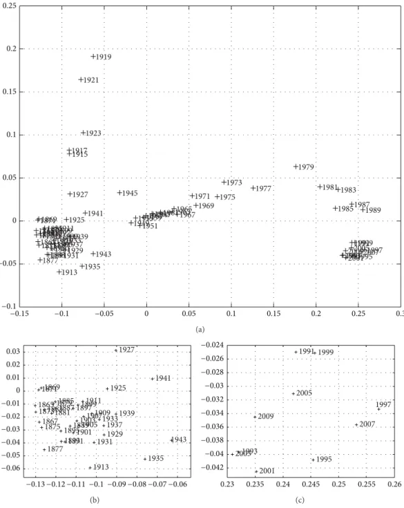
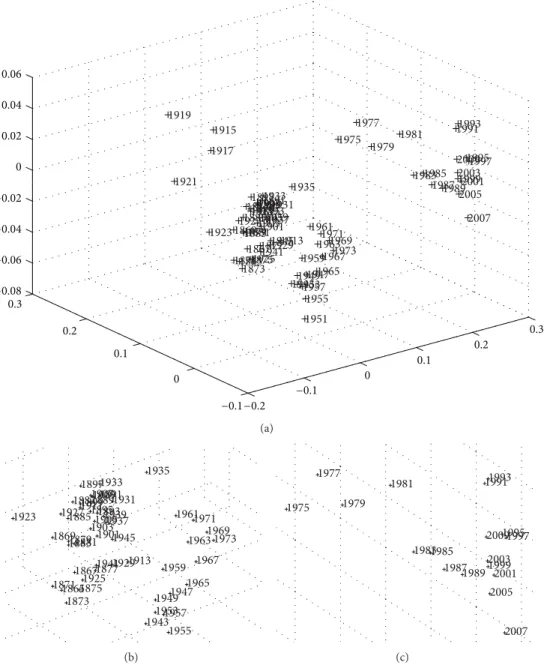
We start by adopting the Cosine correlation𝑟_𝑐as the measure for similarity. It is considered the data within the histori-cal periods𝑇 = {1865–2010, 1867–2010, 1867–2010, 1866– 2010} for sampling periods of ℎ = {2, 3, 4, 5} years, respec-tively. Therefore, we obtain symmetric correlation matrices𝑅 with dimension𝑝 × 𝑝 = {73 × 73, 48 × 48, 36 × 36, 29 × 29}, respectively. The signals over time are vectors with dimension 𝑘_max = 5, whose composition consists of the normalized values for 𝑘 = {GDP, Exports, Imports, Fiscal Revenue, Effective Public Expenditure} where “normalized” means the ratio of the absolute value by the total population at that time. Based on this information, MDS provides the𝑚 = {2, 3} dimensional maps represented in Figures3and4, where the symbol + denotes a point and the numerical label indicates the beginning of the corresponding time period. In other words, only the starting year is depicted, so that the label does not significantly disturb the graphic representation.

The adjustment quality of the MDS fit with these plots is excellent, as can be seen in the Shepard diagrams (Figure 5) and stress plot (Figure 6). We determine that a two-dimen-sional space is appropriate for the mapping because the fitting quality is considerable while representations with higher-dimensional𝑚 add only a marginal improvement.

The exercise is repeated using the Euclidean distance𝑟𝐸 leading to the 3-dimensional map shown in Figure 7. We must observe that at first sight we have a completely different map. Nevertheless, this result is common when varying the measuring index, and, in fact, analyzing MDS maps calls for comparing relative positions and clusters. A detailed visualization of the map confirms the results when using the Cosine correlation. In any event, it is important to reproduce the plot to confirm the robustness of the method in order to draw conclusions.

Shepard diagram and stress test (Figure 8) were also investigated, demonstrating that the 𝑚 = 2-dimensional space is an efficient choice in implementing the fit quality.

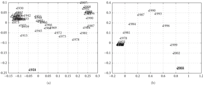
Larger sampling periodsℎ, over approximately the same time length 𝑇, produce a smaller number of points and simpler MDS maps, but the instantaneous nature is gradually replaced by a smoothing averaging over ℎ. Figures 9–11 depict the 2-dimensional MDS maps forℎ = {3, 4, 5}, 𝑇 = {1867–2010, 1867–2010, 1866–2010}, and the indices 𝑟𝐶_and

𝑟𝐸_.

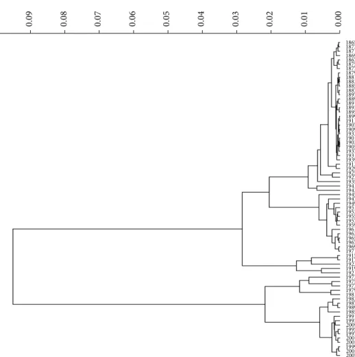
Overall, we obtain the same conclusions as previously, but, as expected, we obtain a compromise between resolution (in time) and simplicity (number of points). Another visual-ization technique is the dendrogram [51], which captures the information content in matrix𝑅 in a different graphic layout.

The dendrogram is a visual representation of the corre-lation between data. The individual spots are arranged along the dendrogram and referred to as leaf nodes. Clusters are formed by joining individual leafs, or leaf clusters, with the join point referred to as a node. The horizontal axis is labelled distance and refers to a distance measure between leafs or leaf clusters. The distance 𝑑 measure between two clusters is calculated as follows: 𝑑 = 1 − 𝑟, where 𝑟 denotes the correlation between leaf clusters.

Figure 12depicts the dendrogram for the case of𝑟𝐶,𝑇 =

1865–2010 and ℎ = 2 years. It is straightforward to compare Figures3,7, and12to conclude that while having the same results, MDS is a good technique for visualizing the informa-tion.

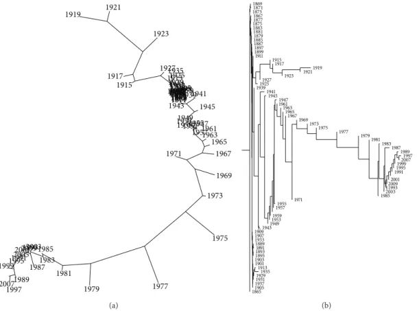
While visual representations are not the main issue addressed in this paper, it is worth mentioning briefly some other visualization techniques. Figures 13and 14 show the trees generated by package Phylip [52] with method “neigh-bor” (options “drawtree” and “drawgram”) and methods “kitsch” and “fitch” (option “drawtree”), respectively. These algorithms produce several types of different trees based on the same correlation matrix, trying to fill the two-dimensional space with an efficient visualization technique. In all cases, we get approximately the same conclusions (since the correlation matrix𝑅 is identical) but with distinct degrees of efficiency.

4. Discussion of the MDS Plots

Three large clusters of periods indicate that the period of the First World War and its aftermath was quite dissimilar from any other period in Portugal. This suggestion is quite accurate for 1915–1925, and particularly for 1915–1921. These were the times of large economic and financial difficulties, and their immediate aftermath [53]. High public expenditure for military purposes plagued Portugal since the beginning. Although joining the Allies only in 1917, military operations were required to protect colonial African territories from German attacks. There were low levels of exportation because of the interruption of land and ocean transportation, and low levels of imports for the same reason, which meant market shortage and disruption, as well as large government rotation [18].

Second World War times were less dramatic and relatively similar to the hardships of Great Depression, a conclusion that is quite plausible for similarity. The Great Depression and the Second World War surely hurted the Portuguese economy in different ways, but historians believe that the large weight of agricultural production and self-sufficiency were positive features that mitigated the effects of inter-national trade decline and commercial closure, with the exception of losses from the decrease of colonial raw-material prices [54]. Although the Allied Victory in the war preserved Portuguese rule over the colonial territories, tropical crops were too abundant during the Depression, and prices fell, as did the contribution of reexportation to the Portuguese balance of payments. In spite of crisis synchronization among industrial countries [55], Portugal’s small participation in

(6)

1865 1867 1869 1871 1873 1875 1877 1879 1881 188318851887 1889 1891 1893 1895 18971899 1901 1903₁₉₀₅19071909 1911 1913 1915 1917 1919 1921 1923 1925 1927 1929 1931 1933 1935 19371939 1941 1943 1945 1947 19491953₁₉₅₁ 1955 1957 195919611963 1965 1967 1969 1971 1973 1975 1977 1979 1981 1983 198519871989 1991 199319951997 1999 2001 2003 2005₂₀₀₇ 2009 −0.15 −0.1 −0.05 0 0.05 0.1 0.15 0.2 0.25 0.3 −0.1 −0.05 0 0.05 0.1 0.15 0.2 0.25 (a) 1865 1867 1869 1871 1873 1875 1877 1879 1881 188318851887 1889 1891 1893 1895 18971899 1901 1903 1905 19071909 1911 1913 1925 1927 1929 1931 1933 1935 1937 1939 1941 1943 −0.13 −0.12 −0.11 −0.1 −0.09 −0.08 −0.07 −0.06 −0.06 −0.05 −0.04 −0.03 −0.02 −0.01 0 0.01 0.02 0.03 (b) 1991 1993 1995 1997 1999 2001 2003 2005 2007 2009 0.23 0.235 0.24 0.245 0.25 0.255 0.26 −0.042 −0.04 −0.038 −0.036 −0.034 −0.032 −0.03 −0.028 −0.026 −0.024 (c)

Figure 3: Two-dimensional MDS map of the Portuguese economic evolution, in the perspective of the Cosine correlation𝑟𝐶,𝑇 = 1865–2010,

andℎ = 2 years. The two charts magnify the two clusters in the left and right lower corners.

the international markets protected the economy from the effects of depressed exportation prices and from the out-come of Atlantic trade disruption due to submarine attacks. Moreover, Portugal remained neutral throughout the conflict, and could even benefit from tungsten exports to both sides of the conflict (Germany and Allies), according to demand opportunities.

These conclusions are important for understanding that such globally difficult times were not much more severe than the traditional nineteenth-century crises. Looking at Figures 3(a)and 13(b), which show the same MSD points

forℎ = 2 years, we may recognize the 1867–1969 crisis, that historians blame on low agricultural production resulting from poor weather conditions, the adverse effects of the Paraguay war on the Portuguese economy, and the knock-on effect of the downturn in the Brazilian economy. Exports to Brazil and emigrants’ remittances from Brazil, which usually contributed to the balance of payments, were now very low [56].

Two clusters identify nineteenth-century times (more visible inFigure 3). The smaller one includes happier peri-ods of large public deficits supported by foreign loans in

(7)

1997 2007 1995 2001 2005 1993 1999 2003 2009 1991 1989 1987 1985 1983 1981 1979 1977 1975 1973 1969 1967 1971 1963 1965 1961 1947 1955 1951 1957 1959 1949 1953 1935 1943 1913 1931 1945 1929 1937 1939 1933 1891 1893 1901 1941 1877 1905 1909 1889 1907 1903 1895 1925 1897 1899 1911 1875 1867 1881 1887 1879 1883 1885 1873 1865 1927 1871 1869 1915 1917 1923 1921 1919 −0.2 −0.1 0 0.1 0.2 0.3 −0.1 0 0.1 0.2 0.3 −0.08 −0.06 −0.04 −0.02 0 0.02 0.04 0.06 (a) 1973 1969 1967 1971 1963 1965 1961 1947 1955 1957 1959 1949 1953 1935 1943 1913 1931 1945 1929 1937 1939 1933 1891 1893 1901 1941 1877 1905 1909 1889 1907 1903 1895 1925 1897 1899 1911 1875 1867 1881 1887 1879 1883 1885 1873 1865 1927 1871 1869 1923 (b) 1997 2007 1995 2001 2005 1993 1999 2003 2009 1991 1989 1987 1985 1983 1981 1979 1977 1975 (c)

Figure 4: Three-dimensional MDS map of the Portuguese economic evolution, in the perspective of the Cosine correlation 𝑟𝐶,𝑇 =

1865–2010, and ℎ = 2 years. The two charts magnify the two clusters in the middle and right sides.

gold-standard times, in which there was easy access to inter-national capital markets to build collective infrastructures, according to the available historical knowledge. This was a public-goods provision policy, dictated by the political blueprint introduced in the 1850s, the so-called Fontismo, evoking the name of the Portuguese politician Ant´onio Maria Fontes Pereira de Melo. Having assumed the positions of ministers of public works, commerce and industry, finance, navy and overseas and having performed the position of prime minister for periods of office, Fontes assumed a special political role in implementing a rail network to foster Portuguese modernization [57].

According toFigure 3, the most dissimilar period in this cloud is the 1873–1875 euphoria. The largest cluster includes

the more difficult crises that are responsible for high gov-ernment rotation, such as the 1875–1877 panic, the 1887–1892 problems that culminated in abandoning the gold-standard (in 1891), and the 1892 sovereign-debt crisis that led to a partial bankruptcy [58]. Currency depreciation increased the debt burden because debt was expressed in foreign currencies and had to be paid with the national depreciated currency, a genuine original sin (as Flandreau and Sussman [59] argue). This partial Portuguese bankruptcy in 1892 consisted of a forced decrease of public debt interest to 1% and a suspension of amortization. It was declared by a government decree on the 13th of June 1892, in the wake of the Baring crisis. The Baring Brothers bank, a traditional lender to the Portuguese government, was suffering from the Argentina and London

(8)

0 0.2 0.4 0.6 0.8 1 0 0.1 0.2 0.3 0.4 0.5 0.6 0.7 0.8 0.9 1 Shepard Original dissimilarities Dis ta n ces/dispa ri ties Distances 1 : 1 line (a) 0 0.2 0.4 0.6 0.8 1 0 0.1 0.2 0.3 0.4 0.5 0.6 0.7 0.8 0.9 1 Shepard Original dissimilarities Dis ta n ces/dispa ri ties Distances 1 : 1 line (b)

Figure 5: Shepard diagrams of the MDS representation of the Portuguese economic evolution, with𝑟𝐶,𝑇 = 1865–2010, and ℎ = 2 years for

the 2d and 3d maps.

1 1.5 2 2.5 3 3.5 4 4.5 5 0 0.01 0.02 0.03 0.04 0.05 0.06 Stress Number of dimensions St re ss

Figure 6: Stress plot of the MDS representation of the Portuguese economic evolution, with𝑟𝐶,𝑇 = 1865–2010, ℎ = 2 years.

crisis, which historians attribute to intensified competition among leaders [58]. Short-run loans from abroad, usually received as floating debt, were no longer available because of the South American crisis. This was coupled with a currency “mismatch,” a twin crisis, which explains why the payment of interest and amortization could not be achieved. Mitchener and Weidenmier [60] document 46 debt defaults by 25 different countries out of roughly 40 to 50 sovereign countries between 1870 and 1913, while Suter [61] counts 72 default episodes between 1820 and 1913, indicating that situations of this kind were widespread, particularly among capital-poor countries throughout the nineteenth century. Soaring public

expenditures and public debt in the nineteenth century are the other face of the rising globalization.

Looking for conclusions for the twentieth century, the large cluster of the 1950s to 1973 in Figure 3describes the most successful period of modern economic growth in Portugal, which was based on budget equilibrium and large exports to the colonial empire in the 1950s, or on small (and disguised) public deficits to support the colonial war, and large exportation to EFTA in the 1960s [18]. According to Smith [62], the establishment of people in the third colonial empire (in Africa), coupled with industrialization, allowed Salazar to balance the budget throughout the four decades

(9)

1865 1867 1869 1871 1873 1875 1877 1879 1881 1883 1885 1887 1889 1891 1893 1895 1897 1899 1901 1903 1905 1907 1909 1911 1913 1915 1917 1919 1921 1923 1925 1927 1929 1931 1933 1935 1937 1939 1941 1943 1945 1947 1949 1951 1953 1955 1957 1959 1961 19631965196719691971197319751977 19791981 1983 1985 1987 198919911993 1995 1997 1999 2001 2003 2005 2007 2009 −0.2 0 0.2 0.4 0.6 0.8 1 1.2 −0.3 −0.2 −0.1 0 0.1 0.2 0.3 0.4

Figure 7: Two-dimensional MDS map of the Portuguese economic evolution, in the perspective of the Euclidean distance𝑟𝐸,𝑇 = 1865–2010,

ℎ = 2 years. 0 0.2 0.4 0.6 0.8 1 0 0.1 0.2 0.3 0.4 0.5 0.6 0.7 0.8 0.9 1 Shepard Original dissimilarities Dis ta n ces/dispa ri ties Distances 1 : 1 line (a) 1 1.5 2 2.5 3 3.5 4 4.5 5 0 0.005 0.01 0.015 0.02 0.025 0.03 Stress Number of dimensions St re ss (b)

Figure 8: Shepard diagram of the two-dimensional and stress plot of the MDS representation of the Portuguese economic evolution with𝑟𝐸,

𝑇 = 1865–2010, and ℎ = 2 years.

of his government and to pay down the public debt that had accumulated from the Fontismo days to the moment before he came to power, and it accounts for the first phase of significant economic growth in Portugal.

Quite apart is the revolutionary period of 1975–1977 in Figures 4(a), 4(c), and 13(a). This period is related to the difficult context of the first oil shock, the 25th April military revolution of Carnations, and decolonization. An increased population (thanks to the half-a-million return flow of people from the empire) and implementation of democracy led to the need for support in the form of the first International Monetary Fund (IMF) loan. According to Figure 3(a), the 1981–1983 crisis is also quite special, and the need for

the second IMF support is usually related to the second oil shock and to political hesitations in designing an economic blueprint for Portugal, after a large communist influence on governance and collective life following the Carnation revolution. Portugal joined Europe and prosperity returned to the Portuguese economy, thanks to economic integration and large budget deficits in a context of easy access to international financial markets for government borrowing.

The special character of the current crisis is clearly visible and identified, as both periods are located quite close and rather distant from any other periods, both in the MDS maps (Figures3,7,9,10, and11), reflecting the high values of budget deficits and government debt, and in consequence of the low

(10)

1867 1870 1873 1876 1879 1882188518911888₁₈₉₄1897 1900 1903 19061909 1912 1915 1918 1921 1924 1927 1930 1933 1936 1939 1942 1945 1948 1951 1954 1957₁₉₆₀ 196319661969 1972 1975 1978 1981 19841987 1990 199319991996 2002 2007 2005 2008 −0.15 −0.1 −0.05 0 0.05 0.1 0.15 0.2 0.25 0.3 −0.25 −0.2 −0.15 −0.1 −0.05 0 0.05 0.1 (a) 1867 1870 1873 1876 1879 1882 1885 1888 1891 1894 1897 1900 1903 1906 1909 1912 1915 1918 1921 1924 1927 1930 1933 1936 1939 1942 1945 1948 1951 1954 1957 196019631966196919721975 1978 1981 1984 1987 1990 1993 1996 1999 2002 2005₂₀₀₈ −0.2 0 0.2 0.4 0.6 0.8 1 1.2 −0.3 −0.2 −0.1 0 0.1 0.2 0.3 0.4 (b)

Figure 9: Two-dimensional MDS maps of the Portuguese economic evolution:𝑇 = 1865–2010, ℎ = 3 years for 𝑟𝐶(a) and𝑟𝐸(b).

−0.25 1867 1871 1875 1879 18831887 1891 1895 18991903 1907 1911 1915 1919 1923 1927 19311935 1939 1943 1947 1951 1955₁₉₅₉ 19631967 1971 1975 1979 19831987 19911999₁₉₉₅ 2003 2007 −0.15 −0.1 −0.05 0 0.05 0.1 0.15 0.2 0.25 0.3 −0.3 −0.2 −0.15 −0.1 −0.05 0 0.05 0.1 (a) 1867 1871 1875 1879 1883 1887 1891 1895 1899 1903 1907 1911 1915 1919 1923 1927 1931 1935 1939 1943 1947 1951195519591963196719711975 1979 1983 1987 1991 1995 1999 2003 2007 −0.2 0 0.2 0.4 0.6 0.8 1 1.2 −0.3 −0.2 −0.1 0 0.1 0.2 0.3 0.4 (b)

Figure 10: Two-dimensional MDS maps of the Portuguese economic evolution:𝑇 = 1867–2010, ℎ = 4 years for 𝑟𝐶(a) and𝑟𝐸(b).

1866 1871 1876₁₈₈₁ 1886 1891 1896 1901₁₉₀₆ 1911 1916 1921 19261931 19361941 19461951 1956 19611966 1971 1976 1981 1986 1991₁₉₉₆ 2001 2006 −0.15 −0.1 −0.05 0 0.05 0.1 0.15 0.2 0.25 0.3 −0.3 −0.25 −0.2 −0.15 −0.1 −0.05 0 0.05 0.1 0.15 (a) 1866 1871 1876 1881 1886 1891 1896 1901 1906 1911 1916 1921 1926 1931 1936 1941 1946 1951 195619611966₁₉₇₁ 1976 1981 1986 1991 1996 2001 2006 −0.2 0 0.2 0.4 0.6 0.8 1 1.2 −0.4 −0.3 −0.2 −0.1 0 0.1 0.2 0.3 (b)

(11)

1865 1873 1871 1869 1867 1875 1877 1879 1881 1883 1885 1887 1897 1889 1891 1893 1895 1899 1911 1907 1909 1933 1901 1903 1905 1937 1931 1939 1913 1929 1925 1927 1935 1941 1943 1945 1947 1949 1951 1953 1955 1957 1959 1961 1963 1965 1967 1969 1971 1915 1917 1923 1919 1921 1973 1975 1977 1979 1981 1983 1987 1989 1985 1991 1993 2009 1995 1997 2001 2003 1999 2005 2007 0.00 0.01 0.02 0.03 0.04 0.05 0.06 0.07 0.08 0.09 0.10

Figure 12: Dendrogram of the Portuguese economic evolution, in the perspective of the Cosine correlation𝑟𝐶,𝑇 = 1865–2010, and ℎ = 2

years, clustering algorithm: unweighted average.

revenues from exports and high cost of imports. Repeating Eichengreen et al. [3], countries may suffer from the original sin of accumulating foreign public debt in globalization, making it very difficult to manage the debt service; an argument that Bordo [4] finds for 30 countries, including Portugal in the period 1880–1914, to conclude on the dramatic character of twin crises (debt and currency crises). This is, again, the special character of the current Portuguese crisis.

Looking at the crises identified we may distinguish those that are more related to balance-of-payments problems from those that are more related to government budget deficits. Balance of payments deficits (as a percentage of GDP) were never as dramatic as they are today. AsFigure 15shows (with deficits in the negative vertical axis), discipline in the balance of payments was the rule from 1865 to the 1990s, with few exceptions.

The first significant imbalance occurred in the nine-teenth-century gold-standard: 5% of GDP in 1891-1892 was enough to require the suspension of convertibility and the exclusion of credit from international capital markets in 1891, followed by the partial bankruptcy of 1892. The sec-ond occurred in 1946-1947, which obliged the Portuguese

government to accept the Marshall Plan offer, even after Salazar’s declared opinion of rejection. The third occurred in 1961, the year the colonial wars began. The last two before the current new-millennium global crisis occurred at the beginning of the democratic regime because of the two oil shocks, requiring two IMF loans. The current situation is the most dramatic in the entire 150-year analysis, as not only did it come in the mid-1990s (and after a recovery it persists throughout the new millennium), but also dipped below 10% of GDP.

To make the picture even darker, the central-state gov-ernment budget mismatch has no parallel in the past, and the First World War was a mild-problem period in comparison with the democracy disarray of 1975–2010, as Figure 16 reveals. As the picture only considers the central state deficit, it is fair to recognize that the real government deficit is not so dramatic because social security and government entrepreneurship sectors are missing here. However, this is the most reliable long-run indicator to preserve homoge-neous historical comparisons.

Political, literary, and philosophical discussions on deca-dency come to the fore of the Portuguese cultural scene whenever severe financial problems afflict the economy. More

(12)

1869 1871 1873 1867187718751883188118871897189918851879 1911 1915 1917 1919 1921 1923 1927 1925 19391941 1945 1947 1961 1963 1965 1967 1969 1973 1975 1977 1979 1981 1983 1987 1989 1997 2007 19991995 199120052001 200919932003₁₉₈₅ 1971 1955 1957 1951 1959 19531949 1943 1909 19071933 18891891 1893 189519031901 19131935 19291931 19371905 1865 (a) 1869 1873 1867 1877 1875 1883 1879 1885 1887 1897 1899 1911 1915 1917 1927 1925 1939 1945 1923 1919 1921 1941 1961 1981 1991 1901 1931 2001 1947 1963 1965 1967 1969 1973 1975 1977 1979 1955 1957 1959 1953 1949 L 1943 1909 1907 1933 1889 1891 1893 1895 1903 1913 1935 1929 1937 1905 1865 1971 1983 1987 1989 1997 2007 1999 1995 | 2009 1 1993 2003 1985 1881 1871 (b)

Figure 13: Trees of the Portuguese economic evolution, in the perspective of the Cosine correlation𝑟𝐶,𝑇 = 1865–2010, ℎ = 2 years, method

“neighbor”, (options “drawtree” and “drawgram”).

than reflecting on such a theme, it is useful to consider that four major periods may be identified throughout the last 150 years, according to the dendrogram and trees and strong Cosine correlation (whileFigure 1timeline considers the main political and financial features).

The 1865–1891 period illustrates how accumulated foreign borrowing led to the end of the gold-standard in 1891, government bankruptcy in 1892, and slow economic growth. These events were a result of irresponsible borrowing to finance the public works that were considered vital for modernization and industrialization, as it was impossible to impose a level of taxation on the population to support such projects. When financial tensions are too harmful for economic growth and social peace, institutional changes may occur, not only accelerating government turnover (making for short and weak governance periods), but also changing the general political and constitutional framework of the country.

The 1892–1925 period: the Portuguese bankruptcy may be considered as an attempt to decrease the weight of public-debt service in the budget, through a decrease of the interest rate in order to reduce it to values close to the rate of GDP growth. Difficult negotiations with lenders for a conversion of the foreign debt lasted until 1902. In spite of a better economic growth, this financial disaster was laid at the feet of the political regime and especially the monarchy, leading

to the victorious Republican Revolution that cast off the royal family and the monarchist regime in 1910. More budget deficits throughout the First World War and the 1920s diffi-culties exacerbated crises, exhausted the Republican political legitimacy, and led to a new political regime that was born in the May 1926 military putsch.

The 1926–1974 Estado Novo financial orthodoxy, with long-term payment of accumulated public debt, required budget control and fiscal system adjustments. They legit-imized this political regime and produced the most impres-sive economic growth path in Portugal’s history, both under Salazar and Caetano’s governance phases [32].

Portuguese democracy, from the 1974 Carnation revolu-tion until today, illustrates the weakness of fiscal politics [63]. Theories on social consent also ask for a serious scientific character for fiscal systems and an image of political honesty (nineteenth-century England, Peel and Gladstone’s efforts to present such an image of the British fiscal system to taxpayers are very well known [64]). In spite of optimistic views on the future of Europe [65], there is a point that political elites may use to convince citizens to accept, or at least tolerate, higher tax burdens [66]. Otherwise, sovereignty alienation or abandoning the Euro may come about, and are high-probability events, at this time.

Some of these considerations may involve ethical, social, and political developments, and, as a result, researchers can

(13)

2005 1999 2007200320011997199520091993 199119891987 19831985 19811979 19771975 1971 1969 1967 1965 19631961195919531957195519511949₁₉₄₇ 1945 1973 1897 1887 1883 1881 1885 1879 1905 1903 1901 1937 1911 1899 1933 1909 1907 1931 1889 1895 1893 1939 1891 1873 1865 1875 1871 1867 1877 1869 1929 1913 1935 1927 1925 1943 1941 1917 1915 1923 1921 1919 (a) 1897189919371911 1935 1931190119031905 1929 1913 1907193319091927 1923 1921 1919 19171915 1943 1949 1947 1965 19992005200720031997199520091993₁₉₉₁ 2001 1989 1987 1985 1983 1981 1979 1977 1975 1973 1971 1969 1963 1967 1961 1955 1959 19511957 1953 1945 1941 1925 1939 1895 1893 1891 188918851887 187918811883 1875 1877 18671873 1871 18691865 (b)

Figure 14: Trees of the Portuguese economic evolution, in the perspective of the Cosine correlation𝑟𝐶,𝑇 = 1865–2010, ℎ = 2 years, methods

“kitsch” and “fitch” (option “drawtree”).

discuss their value due to subjectivity. However, the applied methodology, by adopting quantitative analysis indices and a robust visualization technique, leads to compelling con-clusions, allowing a substantive assessment of the different periods of economic crisis.

5. Conclusions

This paper adopted the MDS analysis for analyzing similarity in business-cycle crises in the Portuguese economy over

the last 150 years. The method proved to be highly efficient and accurate in plotting different clusters of crises and in separating out the current Portuguese difficulties. The final result is a coherent overall picture of the phenomena under consideration.

The current Portuguese crisis will draw out how it will be possible for the country to manage the challenge of maintaining its monetary credibility and, hence, its access to foreign capital [67]. It will also make clear how difficult it is to earn the seal of approval from the powerful central banks of

(14)

Year 1865 1870 1875 1880 1885 1890 1895 1900 1905 1910 1915 1920 1925 1930 1935 1940 1945 1950 1955 1960 1965 1970 1975 1980 1985 1990 1995 2000 2005 2010 15 10 5 0 −5 −10 −15 M o net ar y o p era tio n s/GD P (%)

Figure 15: The balance of payments performance: monetary opera-tions/GDP (sources: before 1998 [25]. For the last years [26,27]).

0.02 0 −0.02 −0.04 −0.06 −0.08 −0.1 −0.12 G o ve rn men t defici t/GD P (%) Year 1865 1870 1875 1880 1885 1890 1895 1900 1905 1910 1915 1920 1925 1930 1935 1940 1945 1950 1955 1960 1965 1970 1975 1980 1985 1990 1995 2000 2005 2010

Figure 16: The government budget performance (surpluses on the positive axis and deficits on the negative axis): government

deficit/GDP (%) (sources: before 1998 [25]. For the last years [26,

27]).

the global economy because of violations of “the rules of the game” resulting from persistent government budget deficits.

Conflict of Interests

The authors of the paper do not have a direct financial relation with any commercial identity mentioned in the paper that might lead to a conflict of interests for any of the authors.

References

[1] F. Capie and G. E. Wood, Eds., Financial Crises and the World

Banking System, McMillan, London, UK, 1986.

[2] C. Kindleberger, Manias, Panics and Crashes: A History of

Financial Crises, John Wiley & Sons, Chichester, UK, 4th

edition, 2000.

[3] B. Eichengreen, R. Hausman, and U. Panizza, “Currency mis-matches, debt intolerance, and original sin: why they are not the same, and why it matters,” NBER Working Paper 10036, 2003. [4] M. Bordo, “Financial crises, 1880–1913: the role of foreign

currency debt,” NBER Working Paper no 11173, 2005.

[5] C. Reinhart and K. S. Rogoff, “Is the 2007 US sub-prime financial crises so different? An international historical compar-ison?” National Bureau of Economic Research, WP 13761, 2008. [6] C. Reinhart and K. S. Rogoff, “Banking crisis: an equal oppor-tunity menace,” National Bureau of Economic Research, WP, 14587, 2008.

[7] C. Reinhart and K. S. Rogoff, “This time is different? A panoramic view of eight centuries of financial crisis,” National Bureau of Economic Research, WP, 13882, 2008.

[8] C. Reinhart and K. S. Rogoff, “From financial crisis to debt crisis,” National Bureau of Economic Research, WP 15795, 2010. [9] J. Tengarrinha, A Historiografia Portuguesa Hoje, HUCITEC,

Lisbon, Portugal, 1999.

[10] C. Betr´an, P. Martin-Ace˜na, and M. Pons, “Financial crises in Spain: lessons from the last 150 years,” DT-AEHE no 1106, 2011. [11] J. Reis, “The historical roots of the modern Portuguese econ-omy: the first century of growth, 1850s to 1950s,” in The New

Portugal: Democracy and Europe, R. Herr, Ed., pp. 126–148,

University of California, Berkeley, Calif, USA, 2003.

[12] P. La´ıns, “O protecionismo em Portugal (1842–1913): um caso mal sucedido de industrialização concorrencial,” Análise Social , vol. 23, no. 97, pp. 481–503, 1987.

[13] M. H. Pereira, Livre câmbio e desenvolvimento económico, Sá da Costa, Lisbon, Portugal, 1983.

[14] D. Justino, A formação do espaço económico nacional, Portugal

1810–1913, Veja, Lisbon, Portugal, 1989.

[15] A. Mateus, Economia Portuguesa: Crescimento no Contexto

Internacional (1910–1998), Verbo, Lisbon, Portugal, 1998.

[16] M. F. Rollo, Ed., Hist´oria da Primeira Rep´ublica Portuguesa, Tinta-da-China, Lisbon, Portugal, 2009.

[17] A. H. O. Marques, A Primeira Rep´ublica Portuguesa, Texto Editores, Lisbon, Portugal, 2010.

[18] L. Amaral, Proximate sources of economic growth in Portugal:

a growth-accounting study for the Portuguese economy [Ph.D. thesis], European University Institute, Florence, Italy, 1997.

[19] J. M. Brito, Industrialização Portuguesa no pós-guerra (1948–

1965): O condicionamento industrial, Dom Quixote, Lisbon,

Portugal.

[20] J. Confraria, “Pol´ıtica industrial do Estado Novo. A regulação dos oligopólios no curto prazo,” Análise Social, vol. 26, no. 112-113, pp. 791–803, 1991.

[21] S. C. Matos, Ed., Crises em Portugal nos s´eculos XIX e XX, Centro de Hist´oria da Universidade de Lisboa, Lisbon, Portugal, 2002. [22] J. T. MacHado, G. M. Duarte, and F. B. Duarte, “Identifying economic periods and crisis with the multidimensional scaling,”

Nonlinear Dynamics, vol. 63, no. 4, pp. 611–622, 2011.

[23] J. T. Machado, F. B. Duarte, and G. M. Duarte, “Analysis of stock market indices through multidimensional scaling,”

Communi-cations in Nonlinear Science and Numerical Simulation, vol. 16,

no. 12, pp. 4610–4618, 2011.

[24] J. A. T. Machado, G. M. Duarte, and F. B. Duarte, “Analysis of financial data series using fractional Fourier transform and

(15)

multidimensional scaling,” Nonlinear Dynamics, vol. 65, no. 3, pp. 235–245, 2011.

[25] N. Val´erio, Ed., Estat´ısticas Hist´oricas Portuguesas, INE, Lisbon, Portugal, 2001.

[26] Instituto Nacional de Estat´ıstica, Anu´arios Estat´ısticos (1998–

2010), Instituto Nacional de Estat´ıstica (INE), Lisbon, Portugal.

[27] Instituto Nacional de Estat´ıstica, Contas Gerais do Estado (1998–

2010), Instituto Nacional de Estat´ıstica (INE), Lisbon, Portugal.

[28] P. La´ıns, Economia Portuguesa no S´eculo XX, Imprensa Nacional Casa da Moeda, Lisbon, Portugal, 1995.

[29] A. Maddison, The World Economy: Historical Statistics, OECD, Paris, France, 2003.

[30] M. Bordo, B. Eichengreen, D. Klingebiel, and M. S. Martinez-Peria, “Is the crisis problem growing more severe?” Economic

Policy, vol. 16, no. 32, pp. 53–82, 2001.

[31] A. B. Nunes, E. Mata, and N. Val´erio, “Portuguese economic growth 1833–1985,” The Journal of European Economic Growth, vol. 18, no. 3, 1989.

[32] M. E. Mata and N. Val´erio, A Concise Economic History of

Portugal, Technical University of Lisbon, Lisbon, Portugal, 2011.

[33] T. Cox and M. Cox, Multidimensional Scaling, Chapman & Hall/CRC, New York, NY, USA, 2nd edition, 2001.

[34] I. Fodor, “A survey of dimension reduction techniques,” Tech. Rep., Center for Applied Scientific Computing, Lawrence Liv-ermore National Laboratory, 2002.

[35] J. Sammon, “A nonlinear mapping for data structure analysis,”

IEEE Transactions on Computers, vol. 18, no. 5, pp. 401–409,

1969.

[36] MathWorks,http://www.mathworks.com/.

[37] W. Martinez and A. Martinez, Exploratory Data Analysis with

MATLAB, Chapman & Hall/CRC, London, UK, 2005.

[38] “The R Project for Statistical Computing,”http://www.r-project

.org/.

[39] J. de Leeuw and P. Mair, “Multidimensional scaling using majorization: SMACOF in R,” Journal of Statistical Software, vol. 31, no. 3, pp. 1–30, 2009.

[40] GGobi, “Interactive and dynamic graphics,”http://www.ggobi

.org/.

[41] J. A. T. Machado and M. E. Mata, Europe at the Crossroads of

Economic Integration: Multidimensional Scaling Analysis of the Period 1970–2010, Économies et Sociétés, Série AF “Histoire

´Economique Quantitative” no. 45, Les Presses de l’ISMEA, 2012. [42] J. B. Kruskal and M. Wish, Multidimensional Scaling, Sage,

Newbury Park, Calif, USA, 1978.

[43] I. Borg and P. J. F. Groene, Modern Multidimensional

Scaling-Theory and Applications, Springer, New York, NY, USA, 2nd

edition, 2005.

[44] S. H. Cha, “Taxonomy of Nominal Type Histogram Distance Measures,” in Proceedings of the American Conference on Applied

Mathematics (MATH ’08), pp. 24–26, Harvard, Mass, USA,

March 2008.

[45] A. V. Korotayev and S. V. Tsirel, “A spectral analysis of world GDP dynamics: Kondratieff waves, kuznets swings, Juglar and Kitchin cycles in global economic development, and the 2008-2009 economic crisis,” Structure and Dynamics, vol. 4, no. 1, pp. 3–57, 2010.

[46] M. Goldstein and P. Turner, Controlling Currency Mismatches

in Emerging Market Economies, Institute of International

Eco-nomics, Washington, DC, USA, 2004.

[47] E. Deza and M. M. Deza, Dictionary of Distances, Elsevier, New York, NY, USA, 2006.

[48] P. J. F. Groenen and P. H. Franses, “Visualizing time-varying correlations across stock markets,” Journal of Empirical Finance, vol. 7, no. 2, pp. 155–172, 2000.

[49] J. Tzeng, H. H. S. Lu, and W. H. Li, “Multidimensional scaling for large genomic data sets,” BMC Bioinformatics, vol. 9, article 179, 2008.

[50] R. N. Shepard, “The analysis of proximities: multidimensional scaling with an unknown distance function—II,”

Psychome-trika, vol. 27, no. 3, pp. 219–246, 1962.

[51] A. Fern´andez and S. G´omez, “Solving non-uniqueness

in agglomerative hierarchical clustering using

multidendrograms,” Journal of Classification, vol. 25, no. 1, pp. 43–65, 2008.

[52] Phylip,http://evolution.genetics.washington.edu/phylip.html.

[53] A. Fishlow, “Lessons from the past—capital markets during the 19th century and the inter-war period,” International

Organiza-tion, vol. 39, pp. 38–93, 1985.

[54] F. Rosas, “A crise de 1929 e os seus efeitos econ´omicos na sociedade Portuguesa,” in O Estado Novo, das origens ao fim da

autarcia 1926–1959, vol. 1, Fragmentos, Lisbon, Portugal, 1987.

[55] M. Bordo and T. Helbling, “International business cycle syn-chronization in historical perspective,” NBER Working Paper no 16103, 2010.

[56] M. H. Pereira, A Pol´ıtica Portuguesa de Emigrac¸˜ao (1850–1930), A Regra do Jogo, Lisbon, Portugal, 1981.

[57] M. E. Mata, “As três fases do fontismo: projectos e realizações,” in Estudos e Ensaios em Homenagem a Vitorino Magalhães

Godinho, S´a da Costa Editora, Lisbon, Portugal, 1988.

[58] M. E. Mata, “Actividade revolucionária no Portugal Contem-porâneo—uma Perspectiva de Longa Duração,” Análise Social, vol. 26, no. 112-113, pp. 755–769, 1991.

[59] M. Flandreau and N. Sussman, “Old sins,” in Other People’s

Money, B. Eichengree and R. Hausmann, Eds., University of

Chicago Press, Chicago, Ill, USA, 2005.

[60] K. J. Mitchener and M. D. Weidenmier, “Supersanctions and sovereign debt repayment,” NBER Working Papers 11472, National Bureau of Economic Research, Inc., 2005.

[61] C. Suter, Debt Cycles in the World Economy—Foreign Loans,

Financial Crises, and Debt Settlements, 1820–1990, Westview

Press, Boulder, Colo, USA, 1992.

[62] G. C. Smith, The Third Portuguese Colonial Empire, a Study in

Economic Imperialism, Manchester University Press,

Manch-ester, UK, 1985.

[63] T. Persson and G. Tabellini, The Effects of Constitutions, MIT Press, Cambridge, Mass, USA, 2003.

[64] M. Daunton, Trusting Leviathan: The Politics of British Taxation

1799–1914, Cambridge University Press, Cambridge, UK, 2001.

[65] B. Eichengreen, “The breakup of the Euro area,” Working Paper

13393, 2007,http://www.nber.org/papers/w13393.

[66] F. S. Mishkin, “Financial policies and the prevention of financial crises in emerging market countries,” in Economic and Financial