Performance of the ATLAS Trigger System in 2015

(1)

EUROPEAN ORGANISATION FOR NUCLEAR RESEARCH (CERN)

Eur. Phys. J. C 77 (2017) 317

DOI:10.1140/epjc/s10052-017-4852-3

CERN-EP-2016-241 30th May 2017

Performance of the ATLAS Trigger System in 2015

The ATLAS Collaboration

During 2015 the ATLAS experiment recorded 3.8 fb−1of proton–proton collision data at a centre-of-mass energy of 13 TeV. The ATLAS trigger system is a crucial component of the experiment, responsible for selecting events of interest at a recording rate of approximately 1 kHz from up to 40 MHz of collisions. This paper presents a short overview of the changes to the trigger and data acquisition systems during the first long shutdown of the LHC and shows the performance of the trigger system and its components based on the 2015 proton– proton collision data.

c

2017 CERN for the benefit of the ATLAS Collaboration.

(2)

1 Introduction

The trigger system is an essential component of any collider experiment as it is responsible for deciding whether or not to keep an event from a given bunch-crossing interaction for later study. During Run 1 (2009 to early 2013) of the Large Hadron Collider (LHC), the trigger system [1–5] of the ATLAS exper-iment [6] operated efficiently at instantaneous luminosities of up to 8 × 1033 cm−2s−1 and primarily at centre-of-mass energies, √s, of 7 TeV and 8 TeV. In Run 2 (since 2015) the increased centre-of-mass en-ergy of 13 TeV, higher luminosity and increased number of proton–proton interactions per bunch-crossing (pile-up) meant that, without upgrades of the trigger system, the trigger rates would have exceeded the maximum allowed rates when running with the trigger thresholds needed to satisfy the physics programme of the experiment. For this reason, the first long shutdown (LS1) between LHC Run 1 and Run 2 opera-tions was used to improve the trigger system with almost no component left untouched.

After a brief introduction of the ATLAS detector in Section2, Section3summarises the changes to the trigger and data acquisition during LS1. Section4gives an overview of the trigger menu used during 2015 followed by an introduction to the reconstruction algorithms used at the high-level trigger in Section5. The performance of the different trigger signatures is shown in Section6for the data taken with 25 ns bunch-spacing in 2015 at a peak luminosity of 5× 1033cm−2s−1with comparison to Monte Carlo (MC) simulation.

2 ATLAS detector

ATLAS is a general-purpose detector with a forward-backward symmetry, which provides almost full solid angle coverage around the interaction point.1 _{The main components of ATLAS are an inner} de-1_{ATLAS uses a right-handed coordinate system with its origin at the nominal interaction point (IP) in the centre of the detector}

(4)

tector (ID), which is surrounded by a superconducting solenoid providing a 2 T axial magnetic field, a calorimeter system, and a muon spectrometer (MS) in a magnetic field generated by three large supercon-ducting toroids with eight coils each. The ID provides track reconstruction within|η| < 2.5, employing a pixel detector (Pixel) close to the beam pipe, a silicon microstrip detector (SCT) at intermediate radii, and a transition radiation tracker (TRT) at outer radii. A new innermost pixel-detector layer, the in-sertable B-layer (IBL), was added during LS1 at a radius of 33 mm around a new and thinner beam pipe [7]. The calorimeter system covers the region |η| < 4.9, the forward region (3.2 < |η| < 4.9) being instrumented with a liquid-argon (LAr) calorimeter for electromagnetic and hadronic measure-ments. In the central region, a lead/LAr electromagnetic calorimeter covers |η| < 3.2, while the hadronic calorimeter uses two different detector technologies, with steel/scintillator tiles (|η| < 1.7) or lead/LAr (1.5 <|η| < 3.2) as absorber/active material. The MS consists of one barrel (|η| < 1.05) and two end-cap sections (1.05 <|η| < 2.7). Resistive plate chambers (RPC, three doublet layers for |η| < 1.05) and thin gap chambers (TGC, one triplet layer followed by two doublets for 1.0 < |η| < 2.4) provide triggering capability as well as (η, φ) position measurements. A precise momentum measurement for muons with|η| up to 2.7 is provided by three layers of monitored drift tubes (MDT), with each chamber providing six to eight η measurements along the muon trajectory. For|η| > 2, the inner layer is instrumented with cathode strip chambers (CSC), consisting of four sensitive layers each, instead of MDTs.

The Trigger and Data Acquisition (TDAQ) system shown in Figure1consists of a hardware-based first-level trigger (L1) and a software-based high-first-level trigger (HLT). The L1 trigger decision is formed by the Central Trigger Processor (CTP), which receives inputs from the L1 calorimeter (L1Calo) and L1 muon (L1Muon) triggers as well as several other subsystems such as the Minimum Bias Trigger Scin-tillators (MBTS), the LUCID Cherenkov counter and the Zero-Degree Calorimeter (ZDC). The CTP is also responsible for applying preventive dead-time. It limits the minimum time between two consec-utive L1 accepts (simple dead-time) to avoid overlapping readout windows, and restricts the number of L1 accepts allowed in a given number of bunch-crossings (complex dead-time) to avoid front-end buf-fers from overflowing. In 2015 running, the simple dead-time was set to 4 bunch-crossings (100 ns). A more detailed description of the L1 trigger system can be found in Ref. [1]. After the L1 trigger ac-ceptance, the events are buffered in the Read-Out System (ROS) and processed by the HLT. The HLT receives Region-of-Interest (RoI) information from L1, which can be used for regional reconstruction in the trigger algorithms. After the events are accepted by the HLT, they are transferred to local stor-age at the experimental site and exported to the Tier-0 facility at CERN’s computing centre for offline reconstruction.

Several Monte Carlo simulated datasets were used to assess the performance of the trigger. Fully simu-lated photon+jet and dijet events generated with Pythia8 [8] using the NNPDF2.3LO [9] parton distri-bution function (PDF) set were used to study the photon and jet triggers. To study tau andb-jet triggers, Z → ττ and t¯t samples generated with Powheg-Box 2.0 [10–12] with the CT10 [13] PDF set and inter-faced to Pythia8 or Pythia6 [14] with the CTEQ6L1 [15] PDF set were used.

3 Changes to the Trigger

/DAQ system for Run 2

The TDAQ system used during Run 1 is described in detail in Refs. [1] and [16]. Compared to Run 1, the LHC has increased its centre-of-mass energy from 8 to 13 TeV, and the nominal bunch-spacing upward. Cylindrical coordinates (r, φ) are used in the transverse plane, φ being the azimuthal angle around the z-axis. The pseudorapidity is defined in terms of the polar angle θ as η= − ln tan(θ/2).

(5)

Level-1 Le ve l-1 A cc ep t Level-1 Muon Endcap

sector logic sector logicBarrel

Level-1 Calo CP (e,γ,τ) CMX JEP (jet, E) CMX Central Trigger MUCTPI L1Topo CTP CTPCORE CTPOUT Preprocessor nMCM Detector Read-Out ROD FE ROD FE ROD FE

...

DataFlow Read-Out System (ROS)

Data Collection Network

Data Storage

Muon detectors Calorimeter detectors

High Level Trigger (HLT) Processors O(28k) RoI Event Data Fast TracKer (FTK) TileCal Accept P ix el /S C T Tier-0

Figure 1: The ATLAS TDAQ system in Run 2 with emphasis on the components relevant for triggering. L1Topo and FTK were being commissioned during 2015 and not used for the results shown here.

has decreased from 50 to 25 ns. Due to the larger transverse beam size at the interaction point (β∗ = 80 cm compared to 60 cm in 2012) and a lower bunch population (1.15× 1011 instead of 1.6× 1011 protons per bunch) the peak luminosity reached in 2015 (5.0× 1033cm−2s−1) was lower than in Run 1 (7.7× 1033 cm−2s−1). However, due to the increase in energy, trigger rates are on average 2.0 to 2.5 times larger for the same luminosity and with the same trigger criteria (individual trigger rates, e.g. jets, can have even larger increases). The decrease in bunch-spacing also increases certain trigger rates (e.g. muons) due to additional interactions from neighbouring bunch-crossings (out-of-time pile-up). In order to prepare for the expected higher rates in Run 2, several upgrades and additions were implemented during LS1. The main changes relevant to the trigger system are briefly described below.

In the L1 Central Trigger, a new topological trigger (L1Topo) consisting of two FPGA-based (Field-Programmable Gate Arrays) processor modules was added. The modules are identical hardware-wise and each is programmed to perform selections based on geometric or kinematic association between trigger objects received from the L1Calo or L1Muon systems. This includes the refined calculation of global event quantities such as missing transverse momentum (with magnitude E_Tmiss). The system was fully installed and commissioned during 2016, i.e. it was not used for the data described in this paper. Details of the hardware implementation can be found in Ref. [17]. The Muon-to-CTP interface (MUCPTI) and the CTP were upgraded to provide inputs to and receive inputs from L1Topo, respectively. In order to better address sub-detector specific requirements, the CTP now supports up to four independent complex dead-time settings operating simultaneously. In addition, the number of L1 trigger selections (512) and

(6)

bunch-group selections (16), defined later, were doubled compared to Run 1. The changes to the L1Calo and L1Muon trigger systems are described in separate sections below.

In Run 1 the HLT consisted of separate Level-2 (L2) and Event Filter (EF) farms. While L2 requested partial event data over the network, the EF operated on full event information assembled by separate farm nodes dedicated to Event Building (EB). For Run 2, the L2 and EF farms were merged into a single ho-mogeneous farm allowing better resource sharing and an overall simplification of both the hardware and software. RoI-based reconstruction continues to be employed by time-critical algorithms. The function-ality of the EB nodes was also integrated into the HLT farm. To achieve higher readout and output rates, the ROS, the data collection network and data storage system were upgraded. The on-detector front-end (FE) electronics and detector-specific readout drivers (ROD) were not changed in any significant way. A new Fast TracKer (FTK) system [18] will provide global ID track reconstruction at the L1 trigger rate using lookup tables stored in custom associative memory chips for the pattern recognition. Instead of a computationally intensive helix fit, the FPGA-based track fitter performs a fast linear fit and the tracks are made available to the HLT. This system will allow the use of tracks at much higher event rates in the HLT than is currently affordable using CPU systems. This system is currently being installed and expected to be fully commissioned during 2017.

3.1 Level-1 calorimeter trigger

The details of the L1Calo trigger algorithms can be found in Ref. [19], and only the basic elements are described here. The electron/photon and tau trigger algorithm (Figure2) identifies an RoI as a 2×2 trigger tower cluster in the electromagnetic calorimeter for which the sum of the transverse energy from at least one of the four possible pairs of nearest neighbour towers (1× 2 or 2 × 1) exceeds a predefined threshold. Isolation-veto thresholds can be set for the electromagnetic (EM) isolation ring in the electromagnetic calorimeter, as well as for hadronic tower sums in a central 2× 2 core behind the EM cluster and in the 12-tower hadronic ring around it. TheET threshold can be set differently for different η regions at a

granularity of 0.1 in η in order to correct for varying detector energy responses. The energy of the trigger towers is calibrated at the electromagnetic energy scale (EM scale). The EM scale correctly reconstructs the energy deposited by particles in an electromagnetic shower in the calorimeter but underestimates the energy deposited by hadrons. Jet RoIs are defined as 4× 4 or 8 × 8 trigger tower windows for which the summed electromagnetic and hadronic transverse energy exceeds predefined thresholds and which surround a 2× 2 trigger tower core that is a local maximum. The location of this local maximum also defines the coordinates of the jet RoI.

In preparation for Run 2, due to the expected increase in luminosity and consequent increase in the num-ber of pile-up events, a major upgrade of several central components of the L1Calo electronics was undertaken to reduce the trigger rates.

For the preprocessor system [20], which digitises and calibrates the analogue signals (consisting of∼7000 trigger towers at a granularity of 0.1× 0.1 in η × φ) from the calorimeter detectors, a new FPGA-based multi-chip module (nMCM) was developed [21] and about 3000 chips (including spares) were produced. They replace the old ASIC-based MCMs used during Run 1. The new modules provide additional flex-ibility and new functionality with respect to the old system. In particular, the nMCMs support the use of digital autocorrelation Finite Impulse Response (FIR) filters and the implementation of a dynamic, bunch-by-bunch pedestal correction, both introduced for Run 2. These improvements lead to a significant rate reduction of the L1 jet and L1Emiss_T triggers. The bunch-by-bunch pedestal subtraction compensates

(7)

Vertical sums ! ! Horizontal sums ! ! ! ! Electromagnetic isolation ring

Hadronic inner core and isolation ring

Electromagnetic calorimeter Hadronic calorimeter Trigger towers ("# × "$ = 0.1 × 0.1) Local maximum/ Region-of-interest

Figure 2: Schematic view of the trigger towers used as input to the L1Calo trigger algorithms.

for the increased trigger rates at the beginning of a bunch train caused by the interplay of in-time and out-of-time pile-up coupled with the LAr pulse shape [22], and linearises the L1 trigger rate as a function of the instantaneous luminosity, as shown in Figure3 for the L1E_Tmisstrigger. The autocorrelation FIR filters substantially improve the bunch-crossing identification (BCID) efficiencies, in particular for low energy deposits. However, the use of this new filtering scheme initially led to an early trigger signal (and incomplete events) for a small fraction of very high energy events. These events were saved into a stream dedicated to mistimed events and treated separately in the relevant physics analyses. The source of the problem was fixed in firmware by adapting the BCID decision logic for saturated pulses and was deployed at the start of the 2016 data-taking period.

The preprocessor outputs are then transmitted to both the Cluster Processor (CP) and Jet/Energy-sum Processor (JEP) subsystems in parallel. The CP subsystem identifies electron/photon and tau lepton candidates withETabove a programmable threshold and satisfying, if required, certain isolation criteria.

The JEP receives jet trigger elements, which are 0.2× 0.2 sums in η × φ, and uses these to identify jets and to produce global sums of scalar and missing transverse momentum. Both the CP and JEP firmware were upgraded to allow an increase of the data transmission rate over the custom-made backplanes from 40 Mbps to 160 Mbps, allowing the transmission of up to four jet or five EM/tau trigger objects per module. A trigger object contains theETsum, η− φ coordinates, and isolation thresholds where relevant.

While the JEP firmware changes were only minor, substantial extra selectivity was added to the CP by implementing energy-dependent L1 electromagnetic isolation criteria instead of fixed threshold cuts. This feature was added to the trigger menu (defined in Section4) at the beginning of Run 2. In 2015 it was used to effectively select events with specific signatures, e.g. EM isolation was required for taus but not for electrons.

Finally, new extended cluster merger modules (CMX) were developed to replace the L1Calo merger modules (CMMs) used during Run 1. The new CMX modules transmit the location and the energy of identified trigger objects to the new L1Topo modules instead of only the threshold multiplicities as done by the CMMs. This transmission happens with a bandwidth of 6.4 Gbps per channel, while the total output bandwidth amounts to above 2 Tbps. Moreover, for most L1 triggers, twice as many trigger selections

(8)

] -1 s -2 cm 30

Instantaneous luminosity / bunch [10

0 0.5 1 1.5 2 2.5 3 3.5 4 4.5 5

Average L1_XE50 rate / bunch [Hz]

0 0.5 1 1.5 2 2.5 ATLAS = 13 TeV s 2015 Data, 50 ns pp Collision Data without pedestal correction with pedestal correction

Figure 3: The per-bunch trigger rate for the L1 missing transverse momentum trigger with a threshold of 50 GeV (L1_XE50) as a function of the instantaneous luminosity per bunch. The rates are shown with and without pedestal correction applied.

and isolation thresholds can be processed with the new CMX modules compared to Run 1, considerably increasing the selectivity of the L1Calo system.

3.2 Level-1 muon trigger

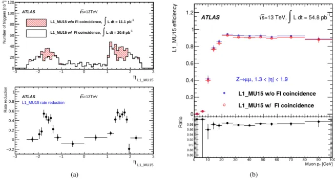
The muon barrel trigger was not significantly changed with respect to Run 1, apart from the regions close to the feet that support the ATLAS detector, where the presence of support structures reduces trigger coverage. To recover trigger acceptance, a fourth layer of RPC trigger chambers was installed before Run 1 in the projective region of the acceptance holes. These chambers were not operational during Run 1. During LS1, these RPC layers were equipped with trigger electronics. Commissioning started during 2015 and they are fully operational in 2016. Additional chambers were installed during LS1 to cover the acceptance holes corresponding to two elevator shafts at the bottom of the muon spectrometer but are not yet operational. At the end of the commissioning phase, the new feet and elevator chambers are expected to increase the overall barrel trigger acceptance by 2.8 and 0.8 percentage points, respectively. During Run 1, a significant fraction of the trigger rate from the end-cap region was found to be due to particles not originating from the interaction point, as illustrated in Figure4. To reject these interactions, new trigger logic was introduced in Run 2. An additional TGC coincidence requirement was deployed in 2015 covering the region 1.3 <|η| < 1.9 (TGC-FI). Further coincidence logic in the region 1.0 < |η| < 1.3 is being commissioned by requiring coincidence with the inner TGC chambers (EIL4) or the Tile hadronic calorimeter. Figure5(a)shows the muon trigger rate as a function of the muon trigger pseudorapidity with and without the TGC-FI coincidence in separate data-taking runs. The asymmetry as a function of η is a result of the magnetic field direction and the background particles being mostly positively charged. In the region where this additional coincidence is applied, the trigger rate is reduced by up to 60% while only about 2% of offline reconstructed muons are lost in this region, as seen in Figure5(b).

(9)

2 4 6 8 10 12 14 m 16 2 4 6 8 10 12 m 0

Large (odd numbered) sectors

BIL BML BOL EEL EIL CSC 1 2 3 4 5 6 EIL4 0 1 2 3 4 5 6 1 2 3 4 5 6 TGCs 1 2 3 4 5 1 2 3 End-cap magnet RPCs y 1 2 TGCs

Large (odd numbered)

EEL EML 2 3 4 5 6 EIL4 3 4 5 6 3 4 5 RPCs 1 2 End-cap toroid z η=2.4 η=1.3 η=1.0 TGC-FI η=1.9 TileCal

Figure 4: A schematic view of the muon spectrometer with lines indicating various pseudorapidity regions. The curved arrow shows an example of a trajectory from slow particles generated at the beam pipe aroundz ∼ 10 m. Triggers due to events of this type are mitigated by requiring an additional coincidence with the TGC-FI chambers in the region 1.3 <_{|η| < 1.9.} L1_MU15 η 3 − −2 −1 0 1 2 3 Number of t rigger s [nb -1] 0 20 40 60 80 100 120 ATLAS s=13TeV -1 L dt = 11.1 pb ∫ L1_MU15 w/o FI coincidence,

-1 L dt = 20.6 pb ∫ L1_MU15 w/ FI coincidence, L1_MU15 η 3 − −2 −1 0 1 2 3 Rate reduction 0.2 − 0 0.2 0.4 0.6 0.8 1 ATLAS s=13TeV

L1_MU15 rate reduction

(a) [GeV/c] T Muon p 0 10 20 30 40 50 60 70 80 90 100 L1_MU15 efficiency 0 0.2 0.4 0.6 0.8 1 1.2 ATLAS s=13 TeV,

∫

L dt = 54.8 pb-1 | < 1.9 η , 1.3 < | µ µ → Z

L1_MU15 w/o FI coincidence L1_MU15 w/ FI coincidence [GeV] T Muon p 0 10 20 30 40 50 60 70 80 90 100 Ratio 0.86 0.88 0.9 0.92 0.94 0.96 0.98 1 (b)

Figure 5: (a) Number of events with an L1 muon trigger with transverse momentum (pT) above 15 GeV (L1_MU15)

as a function of the muon trigger η coordinate, requiring a coincidence with the TGC-FI chambers (open histogram) and not requiring it (cross-hatched histogram), together with the fractional event rate reduction in the bottom plot. The event rate reduction in the regions with no TGC-FI chambers is consistent with zero within the uncertainty. (b) Efficiency of L1_MU15 in the end-cap region, as a function of the pT of the offline muon measured via a

tag-and-probe method (see Section6) usingZ → µµ events with (open dots) and without (filled dots) the TGC-FI coincidence, together with the ratio in the bottom panel.

(10)

4 Trigger menu

The trigger menu defines the list of L1 and HLT triggers and consists of:

• primary triggers, which are used for physics analyses and are typically unprescaled;

• support triggers, which are used for efficiency and performance measurements or for monitoring, and are typically operated at a small rate (of the order of 0.5 Hz each) using prescale factors; • alternative triggers, using alternative (sometimes experimental or new) reconstruction algorithms

compared to the primary or support selections, and often heavily overlapping with the primary triggers;

• backup triggers, with tighter selections and lower expected rate;

• calibration triggers, which are used for detector calibration and are often operated at high rate but storing very small events with only the relevant information needed for calibration.

The primary triggers cover all signatures relevant to the ATLAS physics programme including electrons, photons, muons, tau leptons, (b-)jets and Emiss

T which are used for Standard Model (SM) precision

measurements including decays of the Higgs,W and Z bosons, and searches for physics beyond the SM such as heavy particles, supersymmetry or exotic particles. A set of low transverse momentum (pT)

dimuon triggers is used to collectB-meson decays, which are essential for the B-physics programme of ATLAS.

The trigger menu composition and trigger thresholds are optimised for several luminosity ranges in order to maximise the physics output of the experiment and to fit within the rate and bandwidth constraints of the ATLAS detector, TDAQ system and offline computing. For Run 2 the most relevant constraints are the maximum L1 rate of 100 kHz (75 kHz in Run 1) defined by the ATLAS detector readout capability and an average HLT physics output rate of 1 000 Hz (400 Hz in Run 1) defined by the offline computing model. To ensure an optimal trigger menu within the rate constraints for a given LHC luminosity, prescale factors can be applied to L1 and HLT triggers and changed during data-taking in such a way that triggers may be disabled or only a certain fraction of events may be accepted by them. Supporting triggers may be running at a constant rate or certain triggers enabled later in the LHC fill when the luminosity and pile-up has reduced and the required resources are available. Further flexibility is provided by bunch groups, which allow triggers to include specific requirements on the LHC proton bunches colliding in ATLAS. These requirements include paired (colliding) bunch-crossings for physics triggers, empty or unpaired crossings for background studies or search for long-lived particle decays, and dedicated bunch groups for detector calibration.

Trigger names used throughout this paper consist of the trigger level (L1 or HLT, the latter often omitted for brevity), multiplicity, particle type (e.g. g for photon, j for jet, xe forEmiss_T , te forPE

Ttriggers) and

pTthreshold value in GeV (e.g. L1_2MU4 requires at least two muons withpT> 4 GeV at L1, HLT_mu40

requires at least one muon withpT > 40 GeV at the HLT). L1 and HLT trigger items are written in upper

case and lower case letters, respectively. Each HLT trigger is configured with an L1 trigger as its seed. The L1 seed is not explicitly part of the trigger name except when an HLT trigger is seeded by more than one L1 trigger, in which case the L1 seed is denoted in the suffix of the alternative trigger (e.g. HLT_mu20 and HLT_mu20_L1MU15 with the first one using L1_MU20 as its seed). Further selection criteria (type of identification, isolation, reconstruction algorithm, geometrical region) are suffixed to the trigger name (e.g. HLT_g120_loose).

(11)

4.1 Physics trigger menu for 2015 data-taking

The main goal of the trigger menu design was to maintain the unprescaled electron and single-muon trigger pT thresholds around 25 GeV despite the expected higher trigger rates in Run 2 (see

Sec-tion3). This strategy ensures the collection of the majority of the events with leptonic W and Z boson decays, which are the main source of events for the study of electroweak processes. In addition, compared to using a large number of analysis-specific triggers, this trigger strategy is simpler and more robust at the cost of slightly higher trigger output rates. Dedicated (multi-object) triggers were added for specific ana-lyses not covered by the above. Table1shows a comparison of selected primary trigger thresholds for L1 and the HLT used during Run 1 and 2015 together with the typical thresholds for offline reconstructed ob-jects used in analyses (the latter are usually defined as thepTvalue at which the trigger efficiency reached

the plateau). Trigger thresholds at L1 were either kept the same as during Run 1 or slightly increased to fit within the allowed maximum L1 rate of 100 kHz. At the HLT, several selections were loosened compared to Run 1 or thresholds lowered thanks to the use of more sophisticated HLT algorithms (e.g. multivariate analysis techniques for electrons and taus).

Figures6(a)and6(b)show the L1 and HLT trigger rates grouped by signatures during an LHC fill with a peak luminosity of 4.5× 1033cm−2s−1. The preventive dead-time2The single-electron and single-muon triggers contribute a large fraction to the total rate. While running at these relatively low luminosities it was possible to dedicate a large fraction of the bandwidth to the B-physics triggers. Support triggers contribute about 20% of the total rate. Since the time for trigger commissioning in 2015 was limited due to the fast rise of the LHC luminosity (compared to Run 1), several backup triggers, which contribute additional rate, were implemented in the menu in addition to the primary physics triggers. This is the case for electron,b-jet and Emiss_T triggers, which are discussed in later sections of the paper.

Luminosity block [~ 60s] 300 400 500 600 700 L1 trigger rate [kHz] 0 20 40 60 80 100

120 L1 total Single JET

Single MUON Multi JET

Multi MUON MET

Single EM TAU

Multi EM Combined

ATLAS Trigger Operation

=13 TeV s Data Oct 2015 L1 group rates (with overlaps)

(a) Luminosity block [~ 60s] 300 400 500 600 700 HLT trigger rate [Hz] 0 200 400 600 800 1000 1200 1400 1600 1800 2000

Main Stream Single Jet Tau

Single Muon Multi-Jet Photon

Multi-Muon b-Jet B-Physics

Single Electron MET Combined

Multi-Electron

=13 TeV s Data Oct 2015

HLT group rates (with overlaps)

(b)

Figure 6: (a) L1 and (b) HLT trigger rates grouped by trigger signature during an LHC fill in October 2015 with a peak luminosity of 4.5× 1033cm−2s−1. Due to overlaps the sum of the individual groups is higher than the (a) L1 total rate and (b)Main physics stream rate, which are shown as black lines. Multi-object triggers are included in theb-jets and tau groups. The rate increase around luminosity block 400 is due to the removal of prescaling of the B-physics triggers. The combined group includes multiple triggers combining different trigger signatures such as electrons with muons, taus, jets orEmiss_T .

(12)

Table 1: Comparison of selected primary trigger thresholds (in GeV) at the end of Run 1 and during 2015 together with typical offline requirements applied in analyses (the 2012 offline thresholds are not listed but have a similar relationship to the 2012 HLT thresholds). Electron and tau identification are assumed to fulfil the ‘medium’ criteria unless otherwise stated. Photon andb-jet identification (‘b’) are assumed to fulfil the ‘loose’ criteria. Trigger isolation is denoted by ‘i’. The details of these selections are described in Section6.

Year 2012 2015

√_s

8 TeV 13 TeV

Peak luminosity 7.7× 1033cm−2s−1 5.0× 1033cm−2s−1

pTthreshold [GeV], criteria

Category L1 HLT L1 HLT Offline

Single electron 18 24i 20 24 25

Single muon 15 24i 15 20i 21

Single photon 20 120 22i 120 125

Single tau 40 115 60 80 90

Single jet 75 360 100 360 400

Singleb-jet n/a n/a 100 225 235

Emiss

T 40 80 50 70 180

Dielectron 2×10 2×12,loose 2×10 2×12,loose 15

Dimuon 2×10 2×13 2×10 2×10 11

Electron, muon 10, 6 12, 8 15, 10 17, 14 19, 15

Diphoton 16, 12 35, 25 2×15 35, 25 40, 30

Ditau 15i, 11i 27, 18 20i, 12i 35, 25 40, 30

Tau, electron 11i, 14 28i, 18 12i(+jets), 15 25, 17i 30, 19

Tau, muon 8, 10 20, 15 12i(+jets), 10 25, 14 30, 15

Tau,E_Tmiss 20, 35 38, 40 20, 45(+jets) 35, 70 40, 180

Four jets 4×15 4×80 3×40 4×85 95

Six jets 4×15 6×45 4×15 6×45 55

Twob-jets 75 35b,145b 100 50b,150b 60

Four(Two) (b-)jets 4×15 2×35b, 2×35 3×25 2×35b, 2×35 45

(13)

4.2 Event streaming Luminosity block [~ 60s] 300 400 500 600 700 Rate [Hz] 0 1000 2000 3000 4000 5000

Detector Calibration (partial EB) Trigger Level Analysis (partial EB) Express

Other physics-related Main

=13 TeV s Data Oct 2015 HLT stream rate (a) Luminosity block [~ 60s] 300 400 500 600 700 Bandwidth [MB/s] 0 200 400 600 800 1000 1200 1400

1600 Detector Calibration (partial EB)

Trigger Level Analysis (partial EB) Express

Other physics-related Main

=13 TeV s Data Oct 2015 HLT stream bandwidth

(b)

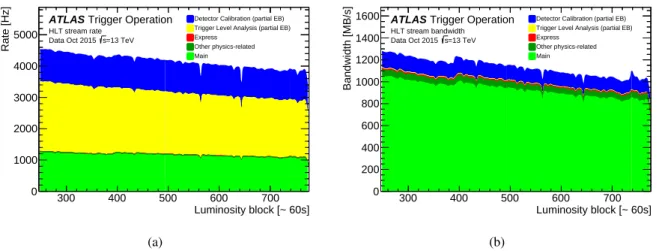
Figure 7: (a) HLT stream rates and (b) bandwidth during an LHC fill in October 2015 with a peak luminosity of 4.5_{× 10}33_cm−2_s−1_{. Partial Event Building (partial EB) streams only store relevant subdetector data and thus have}

smaller event sizes. The other physics-related streams contain events with special readout settings and are used to overlay with MC events to simulate pile-up.

Events accepted by the HLT are written into separate datastreams. Events for physics analyses are sent to a singleMain stream replacing the three separate physics streams (Egamma, Muons, JetTauEtMiss) used in Run 1. This change reduces event duplication, thus reducing storage and CPU resources required for reconstruction by roughly 10%. A small fraction of these events at a rate of 10 to 20 Hz are also written to anExpress stream that is reconstructed promptly offline and used to provide calibration and data quality information prior to the reconstruction of the fullMain stream, which typically happens 36 hours after the data are taken. In addition, there are about twenty additional streams for calibration, monitoring and detector performance studies. To reduce event size, some of these streams use partial event building (partial EB), which writes only a predefined subset of the ATLAS detector data per event. For Run 2, events that contain only HLT reconstructed objects, but no ATLAS detector data, can be recorded to a new type of stream. These events are of very small size, allowing recording at high rate. These streams are used for calibration purposes andTrigger-Level Analysis as described in Section6.4.4. Figure7shows typical HLT stream rates and bandwidth during an LHC fill.

Events that cannot be properly processed at the HLT or have other DAQ-related problems are written to dedicateddebug streams. These events are reprocessed offline with the same HLT configuration as used during data-taking and accepted events are stored into separate data sets for use in physics analyses. In 2015, approximately 339 000 events were written to debug streams. The majority of them (∼ 90%) are due to online processing timeouts that occur when the event cannot be processed within 2–3 minutes. Long processing times are mainly due to muon algorithms processing events with a large number of tracks in the muon spectrometer (e.g. due to jets not contained in the calorimeter). During the debug stream reprocessing, 330 000 events were successfully processed by the HLT of which about 85% were accepted. The remaining 9 000 events could not be processed due to data integrity issues.

(14)

4.3 HLT processing time

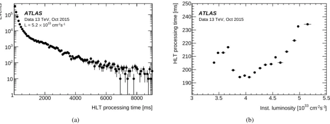
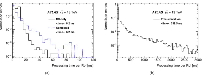
The HLT processing time per event is mainly determined by the trigger menu and the number of pile-up interactions. The HLT farm CPU utilisation depends on the L1 trigger rate and the average HLT pro-cessing time. Figure8shows (a) the HLT processing time distribution for the highest luminosity run in 2015 with a peak luminosity of 5.2×1033cm−2s−1and (b) the average HLT processing time as a function of the instantaneous luminosity. At the highest luminosity point the average event processing time was approximately 235 ms. An L1 rate of 80 kHz corresponds to an average utilisation of 67% of a farm with 28 000 available CPU cores. About 40%, 35% and 15% of the processing time are spent on inner detector tracking, muon spectrometer reconstruction and calorimeter reconstruction, respectively. The muon re-construction time is dominated by the large rate of low-pT B-physics triggers. The increased processing

time at low luminosities observed in Figure8(b)is due to additional triggers being enabled towards the end of an LHC fill to take advantage of the available CPU and bandwidth resources. Moreover, trigger prescale changes are made throughout the run giving rise to some of the observed features in the curve. The clearly visible scaling with luminosity is due to the pileup dependence of the processing time. It is also worth noting that the processing time cannot naively be scaled to higher luminosities as the trigger menu changes significantly in order to keep the L1 rate below or at 100 kHz.

HLT processing time [ms] 2000 4000 6000 8000 Events 1 10 2 10 3 10 4 10 5 10 ATLAS

Data 13 TeV, Oct 2015

-1 s -2 cm 33 10 × L = 5.2 (a) ] -1 s -2 cm 33 Inst. luminosity [10 3 3.5 4 4.5 5 5.5 HLT processing time [ms] 190 200 210 220 230 240 250 ATLAS

Data 13 TeV, Oct 2015

(b)

Figure 8: (a) HLT processing time distribution per event for an instantaneous luminosity of 5.2_{× 10}33_cm−2_s−1_and

average pile-uphµi = 15 and (b) mean HLT processing time as a function of the instantaneous luminosity.

4.4 Trigger menu for special data-taking conditions

Special trigger menus are used for particular data-taking conditions and can either be required for col-lecting a set of events for dedicated measurements or due to specific LHC bunch configurations. In the following, three examples of dedicated menus are given: menu for low number of bunches in the LHC, menu for collecting enhanced minimum-bias data for trigger rate predictions and menu during beam separation scans for luminosity calibration (van der Meer scans).

When the LHC contains a low number of bunches (and thus few bunch trains), care is needed not to trigger at resonant frequencies that could damage the wire bonds of the IBL or SCT detectors, which reside in the magnetic field. The dangerous resonant frequencies are between 9 and 25 kHz for the IBL and above

(15)

100 kHz for the SCT detector. To avoid this risk, both detectors have implemented in the readout firmware a so-called fixed frequency veto that prevents triggers falling within a dangerous frequency range [23]. The IBL veto poses the most stringent limit on the acceptable L1 rate in this LHC configuration. In order to provide trigger menus appropriate to each LHC configuration during the startup phase, the trigger rate has been estimated after simulating the effect of the IBL veto. Figure9 shows the simulated IBL rate limit for two different bunch configurations and the expected L1 trigger rate of the nominal physics trigger menu. At a low number of bunches the expected L1 trigger rate exceeds slightly the allowed L1 rate imposed by the IBL veto. In order not to veto important physics triggers, the required rate reduction was achieved by reducing the rate of supporting triggers.

Number of colliding bunches

500 1000 1500 2000 2500 Rate [kHz] 10 20 30 40 50 60 70 80 90

100 _{ATLAS Operation} _s_{= 13 TeV}

Simulated IBL limit on rate: 72-bunch train-length 144-bunch train-length Expected L1 physics rate

Figure 9: Simulated limits on the L1 trigger rate due to the IBL fixed frequency veto for two different filling schemes and the expected maximum L1 rate from rate predictions. The steps in the latter indicate a change in the prescale strategy. The simulated rate limit is confirmed with experimental tests. The rate limit is higher for the 72-bunch train configuration since the bunches are more equally spread across the LHC ring. The rate limitation was only crucial for the low luminosity phase, where the required physics L1 rate was higher than the limit imposed by the IBL veto. The maximum number of colliding bunches in 2015 was 2232.

Certain applications such as trigger algorithm development, rate predictions and validation require a data set that is minimally biased by the triggers used to select it. This special data set is collected using the en-hanced minimum-bias trigger menu, which consists of all primary lowest-pTL1 triggers with increasing

pT threshold and a random trigger for very high cross-section processes. This trigger menu can be

en-abled in addition to the regular physics menu and records events at 300 Hz for a period of approximately one hour to obtain a data set of around one million events. Since the correlations between triggers are preserved, per-event weights can be calculated and used to convert the sample into a zero-bias sample, which is used for trigger rate predictions during the development of new triggers [24]. This approach requires a much smaller total number of events than a true zero-bias data set.

During van der Meer scans [25], which are performed by the LHC to allow the experiments to calibrate their luminosity measurements, a dedicated trigger menu is used. ATLAS uses several luminosity al-gorithms (see Ref. [26]) amongst which one relies on counting tracks in the ID. Since the different LHC

bunches do not have the exact same proton density, it is beneficial to sample a few bunches at the max-imum possible rate. For this purpose, a minmax-imum-bias trigger selects events for specific LHC bunches and uses partial event building to read out only the ID data at about 5 kHz for five different LHC bunches.

(16)

5 High-level trigger reconstruction

After L1 trigger acceptance, the events are processed by the HLT using finer-granularity calorimeter information, precision measurements from the MS and tracking information from the ID, which are not available at L1. As needed, the HLT reconstruction can either be executed within RoIs identified at L1 or for the full detector. In both cases the data is retrieved on demand from the readout system. As in Run 1, in order to reduce the processing time, most HLT triggers use a two-stage approach with a fast first-pass reconstruction to reject the majority of events and a slower precision reconstruction for the remaining events. However, with the merging of the previously separate L2 and EF farms, there is no longer a fixed bandwidth or rate limitation between the two steps. The following sections describe the main reconstruction algorithms used in the HLT for inner detector, calorimeter and muon reconstruction.

5.1 Inner detector tracking

For Run 1 the ID tracking in the trigger consisted of custom tracking algorithms at L2 and offline tracking algorithms adapted for running in the EF. The ID trigger was redesigned for Run 2 to take advantage of the merged HLT and include information from the IBL. The latter significantly improves the tracking performance and in particular the impact parameter resolution [7]. In addition, provision was made for the inclusion of FTK tracks once that system becomes available later in Run 2.

5.1.1 Inner detector tracking algorithms

The tracking trigger is subdivided intofast tracking and precision tracking stages. The fast tracking consists of trigger-specific pattern recognition algorithms very similar to those used at L2 during Run 1, whereas the precision stage relies heavily on offline tracking algorithms. Despite similar naming the fast tracking as described here is not related to the FTK hardware tracking that will only become available during 2017. The tracking algorithms are typically configured to run within an RoI identified by L1. The offline tracking was reimplemented in LS1 to run three times faster than in Run 1, making it more suitable to use in the HLT. To reduce CPU usage even further, the offline track-finding is seeded by tracks and space-points identified by the fast tracking stage.

5.1.2 Inner detector tracking performance

The tracking efficiency with respect to offline tracks has been determined for electrons and muons. The reconstructed tracks are required to have at least two (six) pixel (SCT) clusters and lie in the region |η| < 2.5. The closest trigger track within a cone of size ∆R = p

(∆η)2_{+ (∆φ)}2 _{= 0.05 of the offline}

reconstructed track is selected as the matching trigger track.

Figure10 shows the tracking efficiency for the 24 GeV medium electron trigger (see Section6.2) as a function of the η and of the pT of the offline track. The tracking efficiency is measured with respect to

offline tracks with pT > 20 GeV for tight offline electron candidates from the 24 GeV electron support

trigger, which does not use the trigger tracks in the selection, but is otherwise identical to the physics trigger. The efficiencies of the fast track finder and precision tracking exceed 99% for all pseudorapidities. There is a small efficiency loss at low pTdue to bremsstrahlung energy loss by electrons.

(17)

η Offline track -3 -2 -1 0 1 2 3 E ff ic ie n c y 0.9 0.92 0.94 0.96 0.98 1 1.02 Precision Tracking Fast Track Finder Precision Tracking Fast Track Finder

_

ATLAS

Data 2015 √s = 13 TeV > 20 GeV T Offline electron track p 24 GeV Electron Trigger

(a) [GeV] T Offline track p 20 30 40 50 60 70 ₁₀2 ₂_×₁₀2 Efficiency 0.9 0.92 0.94 0.96 0.98 1 1.02

PPrreecciissiioonn TTrraacckkiinngg FFaasstt TTrraacckk FFiinnddeerr

ATLAS

Data 2015 √s = 13 TeV > 20 GeV Offline electron track p

T 24 GeV Electron Trigger

_

(b)

Figure 10: The ID tracking efficiency for the 24 GeV electron trigger is shown as a function of the (a) η and (b) pT

of the track of the offline electron candidate. Uncertainties based on Bayesian statistics are shown.

[GeV] T Offline track p 5 678 10 20 30 40 50 102 2×102 E ff ic ie n c y 0.96 0.97 0.98 0.99 1 1.01 1.02 Precision Tracking Fast Track Finder Precision Tracking Fast Track Finder

_

ATLAS

Data 2015 √s = 13 TeV 6 GeV Muon Trigger

(a) [GeV] T 102 Offline track p 5 6 78 10 20 30 40 50 2×102 resolution [mm]₀ d 0.014 0.015 0.016 0.017 0.018 0.019 0.02 0.021 Precision Tracking Fast Track Finder Precision Tracking Fast Track Finder

ATLAS

Data 2015 √s = 13 TeV 6GeV Muon Trigger

_

(b)

Figure 11: The ID tracking performance for the 6 GeV muon trigger; (a) efficiency as a function of the offline recon-structed muonpT, (b) the resolution of the transverse impact parameter,d0as a function of the offline reconstructed

(18)

Figure11(a)shows the tracking performance of the ID trigger for muons with respect to loose offline muon candidates withpT> 6 GeV selected by the 6 GeV muon support trigger as a function of the offline

muon transverse momentum. The efficiency is significantly better than 99% for all pT for both the fast

and precision tracking. Shown in Figure11(b)is the resolution of the transverse track impact parameter with respect to offline as a function of the offline muon pT. The resolution in the fast (precision) tracking

is better than 17µm (15 µm) for muon candidates with offline pT > 20 GeV.

5.1.3 Multiple stage tracking

For the hadronic tau andb-jet triggers, tracking is run in a larger RoI than for electrons or muons. To limit CPU usage, multiple stage track reconstruction was implemented.

A two-stage processing approach was implemented for the hadronic tau trigger. First, the leading track and its position along the beamline are determined by executing fast tracking in an RoI that is fully extended along the beamline (|z| < 225 mm) but narrow (0.1) in both η and φ. (See the blue-shaded region in Figure12.) Using this position along the beamline, the second stage reconstructs all tracks in an RoI that is larger (0.4) in both η and φ but limited to|∆z| < 10 mm with respect to the leading track. (See the green shaded region in Figure 12.) At this second stage, fast tracking is followed by precision tracking. For evaluation purposes, the tau lepton signatures can also be executed in a single-stage mode, running the fast track finder followed by the precision tracking in an RoI of the full extent along the beam line and in eta and phi.

Not reviewed, for internal cir culation only DRAFT [GeV] T Offline track p 5 6 7 8 10 20 30 40 50 ₁₀2 ₁₀2 × 2 Ef ficie n cy 0.96 0.97 0.98 0.99 1 1.01 1.02 Precision Tracking Fast Track Finder Precision Tracking Fast Track Finder ATLAS for approval Data 2015 √s = 13 TeV 6 GeV Muon Trigger

@ (a) [GeV] T Offline p 5 6 7 8 10 20 30 40 50 ₁₀2 ₁₀2 × 2 resolution [mm]₀ d 0.014 0.015 0.016 0.017 0.018 0.019 0.02 0.021 Precision Tracking Fast Track Finder Precision Tracking Fast Track Finder ATLAS for approval Data 2015 √s = 13 TeV 6 GeV Muon Trigger

@

(b)

Figure 11: The ID trigger muon tracking performance is shown with respect to loose muon candidate tracks from the 6 GeV muon trigger with pT>6 GeV; (a) the efficiency versus the offline reconstructed muon pT, (b) the resolution

on the transverse impact parameter, d0versus offline reconstructed muon pT. The offline reconstructed muon tracks

are required to have at least two pixel clusters, and at least six SCT clusters are required to lie in the region |⌘| < 2.5 and pT>6 GeV. The closest matching trigger track within a cone of R < 0.05 of the offline reconstructed track is selected as the matching trigger track. Bayesian uncertainties are shown.

the fast tracking again followed by the precision tracking, but this time in a wider RoI in both ⌘ and , but

397

centred on the z position of the leading track identified by the first stage and limited only to | z| < 10 mm

398

with respect to this leading track. For evaluation purposes, the tau lepton signatures can also be executed

399

in a single-stage mode, running the fast track finder only once in a wide RoI in ⌘ and and extended along

400

the beam line, followed by the precision tracking, again in this wider RoI. The RoIs from these different

401

single-stage and two-stage strategies are illustrated in Fig.12.

402

M Sutton - IDTrigger performance in 13 TeV collisions

TGM 16th September 2015

Understanding the tau timing

2

One-stage tracking RoI

Two-stage tracking: 1st_{stage RoI} Two-stage tracking: 2nd_{stage RoI} Plan view Beam line

• Main saving in time in one-stage tracking comes from narrower φ range in first stage, and narrower z range in second stage

• Narrower η extent in first stage has a smaller impact because of large z extent ! (Beware Δη in the trigger is almost never results in pyramid shaped RoIs - they are nearly always the wedge shapes illustrated here)

• Two stage tracking RoIs not entirely different in volume - FTF timing may not be dissimilar

Figure 12: A schematic illustrating the RoIs from the single-stage and two-stage tau lepton trigger tracking, shown in plan along the transverse direction with the beamline horizontally through the centre of the figure and in perspective view.

Figure13shows the performance of the tau two-stage tracking with respect to the offline tau tracking for

403 27th July 2016 – 16:37 17 beam line Not reviewed, for internal cir culation only DRAFT [GeV] T Offline track p 5 6 7 8 10 20 30 40 50 ₁₀2 ₂_×₁₀2 Ef ficie n cy 0.96 0.97 0.98 0.99 1 1.01 1.02 Precision Tracking Fast Track Finder Precision Tracking Fast Track Finder ATLAS for approval Data 2015 √s = 13 TeV 6 GeV Muon Trigger

@ (a) [GeV] T Offline p 5 6 7 8 10 20 30 40 50 ₁₀2 ₂_×₁₀2 resolution [mm]₀ d 0.014 0.015 0.016 0.017 0.018 0.019 0.02 0.021 Precision Tracking Fast Track Finder Precision Tracking Fast Track Finder ATLAS for approval Data 2015 √s = 13 TeV 6 GeV Muon Trigger

@

(b)

Figure 11: The ID trigger muon tracking performance is shown with respect to loose muon candidate tracks from the 6 GeV muon trigger with pT>6 GeV; (a) the efficiency versus the offline reconstructed muon pT, (b) the resolution

on the transverse impact parameter, d0versus offline reconstructed muon pT. The offline reconstructed muon tracks

are required to have at least two pixel clusters, and at least six SCT clusters are required to lie in the region |⌘| < 2.5 and pT>6 GeV. The closest matching trigger track within a cone of R < 0.05 of the offline reconstructed track is selected as the matching trigger track. Bayesian uncertainties are shown.

the fast tracking again followed by the precision tracking, but this time in a wider RoI in both ⌘ and , but

397

centred on the z position of the leading track identified by the first stage and limited only to | z| < 10 mm

398

with respect to this leading track. For evaluation purposes, the tau lepton signatures can also be executed

399

in a single-stage mode, running the fast track finder only once in a wide RoI in ⌘ and and extended along

400

the beam line, followed by the precision tracking, again in this wider RoI. The RoIs from these different

401

single-stage and two-stage strategies are illustrated in Fig.12.

402

M Sutton - IDTrigger performance in 13 TeV collisions

TGM 16th September 2015

Understanding the tau timing

2

One-stage tracking RoI

Two-stage tracking: 1st_{stage RoI} Two-stage tracking: 2nd_{stage RoI} Plan view beam line

• Main saving in time in one-stage tracking comes from narrower φ range in first stage, and narrower z range in second stage

• Narrower η extent in first stage has a smaller impact because of large z extent ! (Beware Δη in the trigger is almost never results in pyramid shaped RoIs - they are nearly always the wedge shapes illustrated here)

• Two stage tracking RoIs not entirely different in volume - FTF timing may not be dissimilar

Figure 12: A schematic illustrating the RoIs from the single-stage and two-stage tau lepton trigger tracking, shown in plan along the transverse direction with the beamline horizontally through the centre of the figure and in perspective view.

403

27th July 2016 – 16:37 17

Figure 12: A schematic illustrating the RoIs from the single-stage and two-stage tau lepton trigger tracking, shown in plan view (x-z plane) along the transverse direction and in perspective view. The z-axis is along the beam line. The combined tracking volume of the 1st and 2nd stage RoI in the two-stage tracking approach is significantly smaller than the RoI in the one-stage tracking scheme.

tracks withpT > 1 GeV originating from decays of offline tau lepton candidates with pT > 25 GeV, but

with very loose track matching in∆R to the offline tau candidate. Figure13(a)shows the efficiency of

the fast tracking from the first and second stages, together with the efficiency of the precision tracking for the second stage. The second-stage tracking efficiency is higher than 96% everywhere, and improves to better than 99% for tracks with pT > 2 GeV. The efficiency of the first-stage fast tracking has a slower

turn-on, rising from 94% at 2 GeV to better than 99% forpT> 5 GeV. This slow turn-on arises due to the

narrow width (∆φ < 0.1) of the first-stage RoI and the loose tau selection that results in a larger fraction of low-pTtracks from tau candidates that bend out of the RoI (and are not reconstructed) compared to a

(19)

[GeV] T Offline track p 1 2 3 4 5 6 7 10 20 30 102 E ff ic ie n c y 0.9 0.92 0.94 0.96 0.98 1 1.02

Fast Track Finder (Stage 1) Fast Track Finder (Stage 2) Precision Tracking (Stage 2) Fast Track Finder (Stage 1) Fast Track Finder (Stage 2) Precision Tracking (Stage 2) Fast Track Finder (Stage 1) Fast Track Finder (Stage 2) Precision Tracking (Stage 2)

ATLAS

Data 2015 √s = 13 TeV > 1 GeV T offline track p 25 GeV Tau Trigger

_ (a) [GeV] T Oﬄine track p 1 2 3 4 5 6 7 10 20 30 ₁₀2 resolution [mm] 0 d 0.02 0.04 0.06 0.08 0.1 0.12 0.14 0.16 0.18 0.2

Fast Track Finder (Stage 1) Fast Track Finder (Stage 2) Precision Tracking (Stage 2) Fast Track Finder (Stage 1) Fast Track Finder (Stage 2) Precision Tracking (Stage 2) Fast Track Finder (Stage 1) Fast Track Finder (Stage 2) Precision Tracking (Stage 2) ATLAS

Data 2015 √s = 13 TeV > 1 GeV T offline track p 25 GeV Tau Trigger

_

(b)

Figure 13: The ID trigger tau tracking performance with respect to offline tracks from very loose tau candidates withpT > 1 GeV from the 25 GeV tau trigger; (a) the efficiency as a function of the offline reconstructed tau track

pT, (b) the resolution of the transverse impact parameter,d0as a function of the offline reconstructed tau track pT.

The offline reconstructed tau daughter tracks are required to have pT > 1 GeV, lie in the region|η| < 2.5 and have

at least two pixel clusters and at least six SCT clusters. The closest matching trigger track within a cone of size ∆R = 0.05 of the offline track is selected as the matching trigger track.

wider RoI. The transverse impact parameter resolution with respect to offline for loosely matched tracks is seen in Figure13(b)and is around 20µm for tracks with pT > 10 GeV reconstructed by the precision

tracking. The tau selection algorithms based on this two-stage tracking are presented in Section6.5.1. Forb-jet tracking a similar multi-stage tracking strategy was adopted. However, in this case the first-stage vertex tracking takes all jets identified by the jet trigger withET > 30 GeV and reconstructs tracks with

the fast track finder in a narrow region in η and φ around the jet axis for each jet, but with|z| < 225 mm along the beam line. Following this step, the primary vertex reconstruction [27] is performed using the tracks from the fast tracking stage. This vertex is used to define wider RoIs around the jet axes, with |∆η| < 0.4 and |∆φ| < 0.4 but with |∆z| < 20 mm relative to the primary vertex z position. These RoIs are then used for the second-stage reconstruction that runs the fast track finder in the wider η and φ regions followed by the precision tracking, secondary vertexing andb-tagging algorithms.

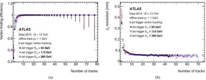
The performance of the primary vertexing in theb-jet vertex tracking can be seen in Figure14(a), which shows the vertex finding efficiency with respect to offline vertices in jet events with at least one jet with transverse energy above 55, 110, or 260 GeV and with no additionalb-tagging requirement. The efficiency is shown as a function of the number of offline tracks with pT > 1 GeV that lie within the boundary of

the wider RoI (defined above) from the selected jets. The efficiency rises sharply and is above 90% for vertices with three or more tracks, and rises to more than 99.5% for vertices with five or more tracks. The resolution inz with respect to the offline z position as shown in Figure14(b)is better than 100µm for vertices with two or more offline tracks and improves to 60 µm for vertices with ten or more offline tracks.

(20)

Number of tracks 10 20 30 40 50 60 70 80 Vertex ﬁ nding e ﬃ ciency 0.2 0.4 0.6 0.8 1 1.2 TTT TTT > 55 GeV > 55 GeV > 55 GeV > 110 GeV> 110 GeV> 110 GeV > 260 GeV> 260 GeV> 260 GeV TTT Jet trigger E Jet trigger E Jet trigger E ATLAS Data 2015 √s = 13 TeV offline track pT> 1 GeV b-jet trigger vertex tracking

_ (a) Number of tracks 0 10 20 30 40 50 60 70 resolution [mm]₀ z 0 0.1 0.2 0.3 0.4 0.5 T T T T T T

> 55 GeV> 55 GeV> 55 GeV > 110 GeV> 110 GeV> 110 GeV > 260 GeV> 260 GeV> 260 GeV T T T Jet trigger E Jet trigger E Jet trigger E ATLAS Data 2015 √s = 13 TeV

offline track pT > 1 GeV

b-jet trigger vertex tracking

_

(b)

Figure 14: The trigger performance for primary vertices in theb-jet signatures for 55, 110 and 260 GeV jet triggers; (a) the vertexing efficiency as a function of the number of offline tracks within the jets used for the vertex tracking, (b) the resolution inz of the vertex with respect to the offline vertex position as a function of the number of offline tracks from the offline vertex.

5.1.4 Inner detector tracking timing

The timing of the fast tracking and precision tracking stages of the electron trigger executed per RoI can be seen in Figure15 for events passing the 24 GeV electron trigger. The fast tracking takes on average 6.2 ms per RoI with a tail at the per-mille level at around 60 ms. The precision tracking execution time has a mean of 2.5 ms and a tail at the per-mille level of around 20 ms. The precision tracking is seeded by the tracks found in the fast tracking stage and hence requires less CPU time.

Processing time per RoI [ms]

0 10 20 30 40 50 60 70 80 90 100 Normalised entries -6 10 -5 10 -4 10 -3 10 -2 10 -1 10 1 ATLAS Data 2015 √s = 13 TeV Tight 24 GeV electron trigger

Fast Track Finder Precision Tracking 0.04 ms ± mean = 6.2 0.02 ms ± mean = 2.5 _

Figure 15: The CPU processing time for the fast and precision tracking per electron RoI for the 24 GeV electron trigger. The precision tracking is seeded by the tracks found in the fast tracking stage and hence requires less CPU time.

The time taken by the tau tracking in both the single-stage and two-stage variants is shown in Figure16. Figure16(a)shows the processing times per RoI for fast tracking stages: individually for the first and second stages of the two-stage tracking, and separately for the single-stage tracking with the wider RoI

(21)

in η, φ andz. The fast tracking in the single-stage tracking has a mean execution time of approximately 66 ms, with a very long tail. In contrast, the first-stage tracking with an RoI that is wide only in thez direction has a mean execution time of 23 ms, driven predominantly by the narrower RoI width in φ. The second-stage tracking, although wider in η and φ, takes only 21 ms on average because of the significant reduction in the RoIz-width along the beam line. Figure 16(b) shows a comparison of the processing time per RoI for the precision tracking. The two-stage tracking executes faster, with a mean of 4.8 ms compared to 12 ms for the single-stage tracking. Again, this is due to the reduction in the number of tracks to be processed from the tighter selection inz along the beam line.

0 50 100 150 200 250 Normalised entries -5 10 -4 10 -3 10 -2 10 -1 10 1 ATLAS Operations Data 2015 √s = 13 TeV Tau trigger: Fast Track Finder

_ _ Two-stage: 1st stage mean = 23.1 ± 0.11 ms Single-stage: mean = 66.2 ± 0.34 ms ___ Two-stage: 2nd stage mean = 21.4 ± 0.09 ms . . .

_

(a)

0 10 20 30 40 50 60 70 80 90 100 Normalised e ntries -5 10 -4 10 -3 10 -2 10 -1 10 1 Two-stage: ___ _{mean = 4.8}_±_{0.04 ms} Single-stage: . . . _{mean = 12.0}_±_{0.07 ms} ATLASOperations Data 2015 √s = 13 TeV

Tau trigger: Precision Tracking _

(b)

Figure 16: The ID trigger tau tracking processing time for (a) the fast track finder and (b) the precision tracking comparing the single-stage and two-stage tracking approach.

5.2 Calorimeter reconstruction

A series of reconstruction algorithms are used to convert signals from the calorimeter readout into objects, specifically cells and clusters, that then serve as input to the reconstruction of electron, photon, tau, and jet candidates and the reconstruction ofEmiss_T . These cells and clusters are also used in the determination of the shower shapes and the isolation properties of candidate particles (including muons), both of which are later used as discriminants for particle identification and the rejection of backgrounds. The reconstruction algorithms used in the HLT have access to full detector granularity and thus allow improved accuracy and precision in energy and position measurements with respect to L1.

5.2.1 Calorimeter algorithms

The first stage in the reconstruction involves unpacking the data from the calorimeter. The unpacking can be done in two different ways: either by unpacking only the data from within the RoIs identified at L1 or by unpacking the data from the full calorimeter. The RoI-based approach is used for well-separated objects (e.g. electron, photon, muon, tau), whereas the full calorimeter reconstruction is used for jets and global event quantities (e.g.Emiss_T ). In both cases the raw unpacked data is then converted into a collection of cells. Two different clustering algorithms are used to reconstruct the clusters of energy deposited in

(22)

the calorimeter, the sliding-window and the topo-clustering algorithms [28]. While the latter provides performance closer to the offline reconstruction, it is also significantly slower (see Section5.2.3). The sliding-window algorithm operates on a grid in which the cells are divided into projective towers. The algorithm scans this grid and positions the window in such a way that the transverse energy contained within the window is the local maximum. If this local maximum is above a given threshold, a cluster is formed by summing the cells within a rectangular clustering window. For each layer the barycentre of the cells within that layer is determined, and then all cells within a fixed window around that position are included in the cluster. Although the size of the clustering window is fixed, the central position of the window may vary slightly at each calorimeter layer, depending on how the cell energies are distributed within them.

The topo-clustering algorithm begins with a seed cell and iteratively adds neighbouring cells to the cluster if their energies are above a given energy threshold that is a function of the expected root-mean-square (RMS) noise (σ). The seed cells are first identified as those cells that have energies greater than 4σ. All neighbouring cells with energies greater than 2σ are then added to the cluster and, finally, all the remaining neighbours to these cells are also added. Unlike the sliding-window clusters, the topo-clusters have no predefined shape, and consequently their size can vary from cluster to cluster.

The reconstruction of candidate electrons and photons uses the sliding-window algorithm with rectangular clustering windows of size∆η×∆φ = 0.075 × 0.175 in the barrel and 0.125 × 0.125 in the end-caps. Since the magnetic field bends the electron trajectory in the φ direction, the size of the window is larger in that coordinate in order to contain most of the energy. The reconstruction of candidate taus and jets and the reconstruction ofEmiss_T all use the topo-clustering algorithm. For taus the topo-clustering uses a window of 0.8× 0.8 around each of the tau RoIs identified at L1. For jets and Emiss_T , the topo-clustering is done for the full calorimeter. In addition, theEmiss_T is also determined based on the cell energies across the full calorimeter (see Section6.6).

5.2.2 Calorimeter algorithm performance

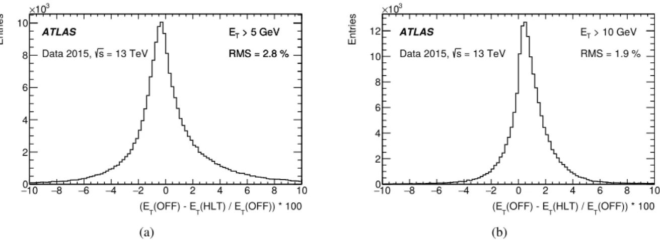
The harmonisation between the online and offline algorithms in Run 2 means that the online calorimeter performance is now much closer to the offline performance. The ET resolutions of the sliding-window

clusters and the topo-clusters with respect to their offline counterparts are shown in Figure 17. The ET

resolution of the sliding-window clusters is 3% for clusters above 5 GeV, while the ET resolution of

the topo-clustering algorithm is 2% for clusters above 10 GeV. The slight shift in cell energies between the HLT and offline is due to the fact that out-of-time pile-up effects were not corrected in the online reconstruction, resulting in slightly higher reconstructed cell energies in the HLT (this was changed for 2016). In addition, the topo-cluster based reconstruction shown in Figure17(b)suffered from a mismatch

of some calibration constants between online and offline during most of 2015, resulting in a shift towards lower HLT cell energies.

5.2.3 Calorimeter algorithm timing

Due to the optimisation of the offline clustering algorithms during LS1, offline clustering algorithms can be used in the HLT directly after the L1 selection. At the data preparation stage, a specially optimised infrastructure with a memory caching mechanism allows very fast unpacking of data, even from the full calorimeter, which comprises approximately 187 000 cells. The mean processing time for the data

(23)

(OFF)) * 100 T (HLT) / E T (OFF) - E T (E 10 − −8 −6 −4 −2 0 2 4 6 8 10 Entries 0 2 4 6 8 10 3 10 × ATLAS = 13 TeV s Data 2015, > 5 GeV T E RMS = 2.8 % > 5 GeV T E RMS = 2.8 % (a) (OFF)) * 100 T (HLT) / E T (OFF) - E T (E 10 − −8 −6 −4 −2 0 2 4 6 8 10 Entries 0 2 4 6 8 10 12 3 10 × ATLAS = 13 TeV s Data 2015, > 10 GeV T E RMS = 1.9 % (b)

Figure 17: The relative differences between the online and offline ETfor (a) sliding-window clusters and (b)

topo-clusters. Online and offline clusters are matched within ∆R < 0.001. The distribution for the topo-clusters was obtained from the RoI-based topo-clustering algorithm that is used for online tau reconstruction.

preparation stage is 2 ms per RoI and 20 ms for the full calorimeter, and both are roughly independent of pile-up. The topo-clustering, however, requires a fixed estimate of the expected pile-up noise (cell energy contributions from pile-up interactions) in order to determine the cluster-building thresholds and, when there is a discrepancy between the expected pile-up noise and the actual pile-up noise, the processing time can show some dependence on the pile-up conditions. The mean processing time for the topo-clustering is 6 ms per RoI and 82 ms for the full calorimeter. The distributions of the topo-clustering processing times are shown in Figure18(a) for an RoI and Figure18(b) for the full calorimeter. The RoI-based topo-clustering can run multiple times if there is more than one RoI per event. The topo-clustering over the full calorimeter runs at most once per event, even if the event satisfied both jet andEmiss

T selections at

L1. The mean processing time of the sliding window clustering algorithm is not shown but is typically less than 2.5 ms per RoI.

Processing time per call [ms]

2 4 6 8 10 12 14 16 18 20 Entries 0 5 10 15 20 25 30 35 40 45 50×103 ATLAS = 13 TeV s Data 2015, <t> = 5.7 ms (a)

Processing time per call [ms] 0 20 40 60 80 100 120 140 160 180 200 220 Entries 0 1 2 3 4 5 6 7 8 9×103 ATLAS = 13 TeV s Data 2015, <t> = 82 ms (b)

Figure 18: The distributions of processing times for the topo-clustering algorithm executed (a) within an RoI and (b) on the full calorimeter. The processing times within an RoI are obtained from tau RoIs with a size of∆η × ∆φ = 0.8× 0.8.