Operational asset replacement strategy : a real options approach

WORKING PAPER SERIES

CEEAplA WP No. 01/2009

Operational Asset Replacement Strategy

A Real Options Approach

João Zambujal João Duque

Operational Asset Replacement Strategy

A Real Options Approach

João Zambujal

Universidade da Madeira(DGE)

João Duque

Universidade Técnica de Lisboa (ISEG)

RESUMO/ABSTRACT

Operational Asset Replacement Strategy A Real Options Approach

This article analyses the problem of replacement by investigating the optimal moment of investment replacement in a given tax environment with a given depreciation policy. An operation and maintenance cost minimization model, based on the definition of equivalent annual cost, is applied to a real options paradigm. The developed methodology allows for an innovative evaluation of the flexibility of replacement process analysis. A new two- factor evaluation function is introduced to quantify decisions of asset replacement under a unique cycle environment. This study improves upon previous findings in the literature as it accounts for autonomous salvage value processes. Based on partial differential equations, this model achieves a general analytical solution and particular numerical solution. The results differ significantly from those observed in one-factor models by showing evidence of over-evaluation in optimal levels of replacement, and by confirming suspicions that different types of uncertainties produce non-monotonous effects on the optimal replacement level. The scientific contribution of this study lies in new and stronger approaches to equivalent annual cost literature, supplying an algorithm for operation and maintenance cost minimization that is conditioned by autonomous salvage value. This study also contributes to the real options literature by developing of a two-factor model with Brownian processes applied to asset replacement. JEL classifications: D81, D92, H25

Keywords: Replacement, Real Options, Uncertainty, Equivalent Annual Cost, First Passage Time.

João Zambujal

Departamento de Gestão e Economia Universidade da Madeira

Campus da Penteada 9050-590 Funchal, Portugal João Duque

Instituto Superior de Economia e Gestão Universidade Técnica de Lisboa

Rua Miguel Lupi, 20, 1249-078 Lisboa, Portugal

A Real Options Approach

January, 2009

João Z. Oliveira

Department of Management and Economics University of Madeira Campus da Penteada 9050-590 Funchal, Portugal Tel: (351) 917 267 681 Fax: (351) 291 705 040 Email: jzo@uma.pt

João C. Duque

Institute of Economics and Management (ISEG) Technical University of Lisbon

Rua Miguel Lupi, 20, 1249-078 Lisboa, Portugal

Tel: (351) 213 925 800 Fax: (351) 213 922 808 Email: jduque@iseg.utl.pt

Operational Asset Replacement Strategy

A Real Options Approach

Abstract: This article analyses the problem of replacement by investigating the optimal moment of investment replacement in a given tax environment with a given depreciation policy. An operation and maintenance cost minimization model, based on the definition of equivalent annual cost, is applied to a real options paradigm. The developed methodology allows for an innovative evaluation of the flexibility of replacement process analysis. A new two- factor evaluation function is introduced to quantify decisions of asset replacement under a unique cycle environment. This study improves upon previous findings in the literature as it accounts for autonomous salvage value processes. Based on partial differential equations, this model achieves a general analytical solution and particular numerical solution. The results differ significantly from those observed in one-factor models by showing evidence of over-evaluation in optimal levels of replacement, and by confirming suspicions that different types of uncertainties produce non-monotonous effects on the optimal replacement level. The scientific contribution of this study lies in new and stronger approaches to equivalent annual cost literature, supplying an algorithm for operation and maintenance cost minimization that is conditioned by autonomous salvage value. This study also contributes to the real options literature by developing of a two-factor model with Brownian processes applied to asset replacement.

JEL classifications: D81, D92, H25

Keywords: Replacement, Real Options, Uncertainty, Equivalent Annual Cost, First Passage Time.

1.

Introduction

The traditional analysis for the selection of the optimal replacement level employs the minimum Equivalent Annual Cost (EAC) determination. This methodology implies the calculation of a cost series for current and alternative assets. The method may also consider a depreciation tax shelter, a cost of postponing replacement to the next year and a asset replacement. Assuming an infinite time horizon, the replacement cycle will correspond to the minimum cost. Among other assumptions, the traditional methodology also assumes a similar Operation and Maintenance Cost (OMC) structure for future replacement assets, a known salvage value, and certainty in tax policy. One of the major problems of the replacement decision evaluation method is not considering uncertainty, implicitly or explicitly.

To address these problems, Rust (1985) suggests that a greater OMC value indicates higher asset deterioration. Rust (1985) described the OMC evolution as an arithmetic Brownian motion with constant drift and constant volatility. Ye (1990) continues this analysis of the replacement problem by considering OMC as an Itô process. This approach implies that OMC returns to an initial state each time a replacement occurs. Ye’s (1990) article influences the Mauer and Ott (1995) model through the introduction of a geometric Brownian motion (GBM) to modulate OMC. Ye (1990) also assumes a physical deterioration that increases stochastically.

2.

A Two-factor Replacement Model

This paper considers that salvage value is as uncertain as its OMC; when asset replacement occurs, the salvage value can be different than previous estimates. The modulation of salvage value with a geometric Brownian motion

(GBM) will produce a different relationship between OMC

( )

C and salvage value

( )

S , from which a new optimal replacement level results. Our model considers a firm operating at a fixed level of output with two geometric Brownian motions, one for C and another for S :

C C C

dC=α Cdt+σ Cdz , (1)

S S S

dS =α Sdt+σ Sdz , (2)

with instantaneous drifts α_C ≥0,α_S ≤0 and instantaneous volatilities 0, 0

C S

σ ≥ σ ≥ . This model also assumes two stochastic equivalent assets for which the initial OMC CN ≥0 and the initial salvage valueSN >0 evolve

according to equations (1) and (2). This section examines how the modification of the salvage value framework affects the optimal replacement level. Other assumptions of this model are (1) that there is a single asset at a given time, and (2) that production does not expand or contract.

Therefore, when OMC reaches a certain level, the current asset sale occurs and is replaced by another stochastically equivalent asset. So, one has a cost minimization problem to determine the optimal replacement level using a two-factor model. With rf being the risk free rate, V C t

(

t,

)

corresponds to the

expected discounted OMC:

(

)

(

(

)

( )

)

0 , min 1 f t r t a t t C V C t E C τ τδ ϑ t e dt ∞ −   =  − −  

∫

. (3)

From the previous expression, the cost flow results from subtracting after-tax OMC Ct

(

1−τ

)

from the tax shield

( )

a

t

OMC as described in (3),τ is the tax rate,

δ

a corresponds to the depreciation rate and ϑ

( )

t indicates the book value given by:

( )

t P

(

1

)

e δat

ϑ

_{= −}

ϕ

−

, (4)

where P is the acquisition price and ϕ is the investment tax credit rate. One can see from (3) that there is a functional dependence of V

( )

. on both Ct and t.. As

we have two variables

(

C tt,

)

, problem simplification justifies the adoption of an

infinite horizon time framework, relaxing V

( )

. from the dependence of t.

Assuming the distribution of risks associated with OMC by financial assets and using the contingent claims approach, the exchange option Exc C S

(

,

)

must satisfy the following equation (Merton, 1973):

(

2 2 2 2

) (

)

(

)

1

2

2 ExcCCσCC + ExcCSσ σC SCSρCS +ExcSSσSS + rf −δC Exc CC + rf −δS Exc SS =r Excf (5)

with the risk-adjusted drift rate of cost *

C rf C

α = −δ , the risk-adjusted drift rate of salvage value *

S rf S

α = −δ , and the risk-free rate of interest rf. The convenience

yields of each stochastic variable are represented by

δ

C and

δ

S.

From equation (5) and according to Appendix A, the general solution is derived from:

(

)

2 1 2 , a S S C k b c S Exc C S k C k C C α ω ω σ σ     _{ } =_{  } + _     , (6)

where ka, kb, and kc are constants, and w1 and w2 represent the roots of a

quadratic equation derived in Appendix A and given by (29).

To determine the solution to the replacement problem, one must calculate the three constants ki and the replacement critical level

(

)

* *

,

C S . In order to achieve this, equation (6) must satisfy five boundary conditions.

The right to acquire an asset at the exercise price of selling the other asset describes a long position on an exchange option. The same exchange option can be seen as the right to sell an asset at the exercise price of buying the other asset. In order to determine

(

C S*, *

)

, the following boundary conditions should be applied. The first one implies its satisfaction by Exc C S

(

*, *

)

upon the replacement level.

(

* *

) ( ) (

* * *

)

, , Exc C S =V C − Ω C S , (7) where

( )

( )

(

)

(

)

( )

* * * * * 2 1 1 1 1 2 a N f C f C C C P V C C C r _r ξ ξ δ τ ϕ τ α _{α ξ ξσ} −    ₋   ₋  =_ _ −  − _{ }   _{− − −}   , (8) and

(

* *

)

( )

(

)

*

(

*

( )

*

)

, _N 1 C S V C P ϕ S τ S ϑ C  Ω = + − −_ − − ⌢ _ . (9)

At the critical level

(

C S*, *

)

, the exchange option value Exc C S

(

*, *

)

must equal the difference between the expected discounted value of after-tax OMC and the total alternative cost value Ω

(

C S*, *

)

. The value Ω

(

C S*, *

)

reflects the

sum of the expected discounted value of after-tax OMC in the instant after replacement, with the net acquisition price of a alternative asset P

(

1−ϕ

)

minus the after tax salvage value (salvage value *

S minus capital gains tax

( )

(

* *

)

S C

τ −ϑ⌢

).

Equations (10) and (11) must ensure that the smooth past condition is satisfied (Dixit and Pindyck, 1994). In conjunction with other conditions, the presented boundary conditions permit the determination of three constants, which exist in (6). Therefore, the value function in equation (6) must satisfy the following equations:

(

* *

) ( )

*

(

* *

)

, , C C C E C S =V C − Ω C S , (10)

(

* *

) ( )

*

(

* *

)

, , S S S E C S =V C −Ω C S , (11)

Condition (12) describes the function’s Exc C S

(

,

)

behavior when the OMC approaches the minimal allowed value CN. Thus, when C assumes values next

to CN, the probability of C grows until *

C is very low, significantly diminishing the probability of asset replacement. As such, the value of the exchange option

(

,

)

Exc C S will tend towards zero:

(

)

lim , 0

N

C−>C Exc C S = , (12)

When OMC becomes very high relative to the savage value S , the increase in value of the exchange option should equal the savings gained between the OMC of the current asset and the OMC of the alternative asset:

( )

( )

C C N

resulting in the following condition:

(

)

( )

( )

lim C , C C N

C−>∞Exc C S =V C −V C . (13)

When *

C goes up, the savage value must go down to make the replacement economically viable. As time goes by, the OMC must go up in order to justify the capital cost originating from asset replacement.

As a base to our solution, the numerical case belonging to Mauer and Ott (1995) will be revisited, corrected, and prepared for this model.

3.

Description of the numerical case

Before continuing with our solution through modeling, the numerical case, which was specifically designed to test critical asset replacement solutions, should be described. Because the results of this numerical case are going to serve as a comparison for the new model, all previous parameter values, with the exception of

α

C, have been accepted. Relative to

α

C, we initially consider a

growth rate

α

_C =0.15 and a volatility

σ

_C =0.10. As the value of

α

C is greater

than the discount rate r_f =0.07, by Gordon’s Model, one considers α_C =0.06.

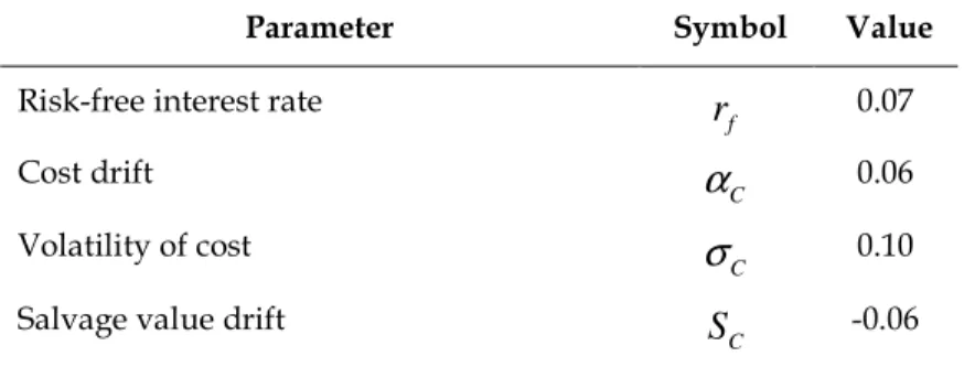
Table 1: Set of parameters and values of the numerical case

Parameter Symbol Value

Risk-free interest rate

f r 0.07 Cost drift C

α

0.06 Volatility of cost C

σ

0.10

Salvage value drift

C

Volatility of salvage value

C

S 0.10

Market risk price η 0.4

Minimal cost

N

C 1

Acquisition price P 10

Investment tax credit rate ϕ 0

Tax rate

τ

0.30

Depreciation rate

δ

a _0.50

Mun (2003) presents a case with

α

_C =0.10 and

σ

_C =0.35 where

σ α

_{C C} =3.5. For

α

_C =0.06, one obtains

σ α

_{C C} =1.66, which is a satisfactory 50% of Mun’s (2003) previous ratio.

To make the risk adjustment, we use the Shape ratio as the risk price. Bernstein and Damodaran (1998) and Hull (1993) describe this concept as the premium demanded by the market to compensate for each unit of risk. Taking the total risk premium to equal η σ ρm C Cm, the adjusted growth rate value

* C α will be: * C C m C Cm

α

=

α η σ ρ

− . (14)

We estimate the market risk price to be η_m =0.40, which is based on the use of a market index return rate as an evaluation pattern. Therefore, the market risk price is calculated as the ratio between the market risk premium

µ

m−rf and the

market standard deviationσm:

m f m m r µ η σ − = . (15)

According to Ibbotson Associates (2006), the market risk premium for this case is

(

µ

_m−r_f

)

=0.08and volatility is

σ

_m =0.2. These values result in a market risk price of

η

_m=0.40. The lack of correlation between the OMC and the systematic factor of evaluation, which produces an adjusted growth rate *

C

α

with an annual value of 0.06, is assumed. Concerning new asset characteristics, an acquisition price P =10 and OMC initial value C_N =1

is also assumed. Thus,

( )

N

V C corresponds to the after-tax value of the cost to replace an infinite sequence of stochastic assets. In respect to tax parameters, the numerical case includes a credit investment rate, whose value represents the possibility of reinvestment of the amount resulting from an asset sale, and the case also defines an initial value ϕ=0, a tax rate τ =0.30, and a depreciation rate δa

=0.50. The depreciation method follows a negative exponential function. In discrete terms, exponential amortization corresponds to a regimen similar to the one described in Table 2.

Table 2: Description of the depreciation rate for annual periods

Period 1 2 3 4 5

Depreciation Rate 39.35% 23.87% 14.47% 8.78% 5.33%

4.

Characteristics of the solution

The OMC critical level is endogenous and results from equation (6) in conjunction with the applied boundary conditions defined in the previous section. The numerical simulation obtained from the present model produced critical value results in Table 3.

Table 3: Numerical solution for a two-factor function1

Mod. C* S* E[T*] V(C*) V(CN)

0 2,736 2,924 6,700 23,960 22,835

1 2,264 3,534 13,202 23,032 15,507

2 1,137 5,999 1,085 82,184 78,325

From Table 3, a substantial critical level modification is possible. This could be due to the introduction of decreasing dynamics for salvage value S that could motivate an anticipation of asset replacement. A more detailed observation highlights an even larger variation in the replacement period, which results from the application of the critical level to a first passage time distribution. These results seem to confirm the intuition that the introduction of a two-factor function would induce strong variations in the cost replacement critical level, confirming some weaknesses in the previous model. These indications lead us to conduct a comparative analysis based on behavioral standards and also to conduct an analysis of the impact of variations of each parameter in the determination of the optimal replacement policy.

5.

Sensitivity analysis

This section examines the impact of changes in parameter values on the replacement model by analyzing replacement boundary values and the optimal replacement periods for different states of nature. In this way, one can defines a set of panels to isolate the effect of varying each parameter and verify the critical level sensitivity associated with parameter value variations.

The analysis begins with observation of the impact of varying parameters constituting the salvage value S , described in equation (2). Table 4 shows the critical level and critical period updates resulting from the variation of drift rate

S

α

.

Table 4: Effect of increasing the cost growth rate ααααs C* S* E[T*] V(C*) V(CN) -0.09 1.079 6.501 0.940 90.290 83.254

-0.06 1.137 5.999 1.085 82.184 78.325

-0.03 1.157 5.218 1.328 83.189 78.325

Elevating αS results in two positive effects resulting from changing these

parameter: 1) an increase in the critical OMC, and 2) reduction in the exercise period. The intuitive explanation for this effect resides in the more distant intersection point associated from a flatter slope. The effect of changing

σ

S

(shown in Table 5 at 0.05 intervals) will depend on its relative position to

σ

C. If

C S

σ

>

σ

, the critical level should go down and if

σ

C ≤

σ

S the critical level should

go up.

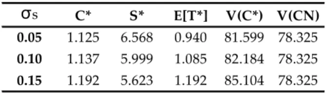
Table 5: Effect of changing the standard deviation of salvage value

σ_{s C* S* E[T*] V(C*) V(CN)}

0.05 1.125 6.568 0.940 81.599 78.325

0.10 1.137 5.999 1.085 82.184 78.325

0.15 1.192 5.623 1.192 85.104 78.325

From Table 5, one can verify an ascent of *

C coincident with *

E T _{ }. As expected, the introduction of

σ

S does not significantly modify the function of the

replacement model but induces a lower replacement critical level. Table 5 also shows that the simple consideration of

σ

S results in a 10.7% decrease in a new

critical *

C compared to the adjusted numerical case. The reason for this behavior seems to be in the evidence that less volatile markets create fewer investment opportunities based on economic savings from asset replacement.

As Dobbs (2002) and Dixit (1989) suggest, volatility in variation intervenes with the value of the asset exchange option. In this case, the exchange option becomes influenced not only by

σ

C but also by

σ

S, whose increase provokes a

delay in the moment that the asset exchange option is chosen. Uncertainty in S

produces a new optimal boundary where σS and σC work against each other.

An increase in

σ

Scan induce the decision to replace by increasing the possibility

of a future price decline, while an increase in

σ

C induces a choice to keep the

asset because future OMC are expected to descend. Thus, delay or advancement of the optimal replacement moment will depend on the combined effect of these two volatilities (Brach, 2002).

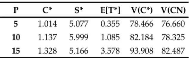
The next table shows the two-factor function panel with the effect from varying the acquisition price P. In the previous tests, the varying P upwards led to an increase in *

C , establishing a higher level for exercising the replacement option. This panel establishes positive and negative variations about the acquisition price using a standard level of P=10, which results in the following:

Table 6: Effect of changing the acquisition price

P C* S* E[T*] V(C*) V(CN)

5 1.014 5.077 0.355 78.466 76.660

10 1.137 5.999 1.085 82.184 78.325

15 1.328 5.166 3.578 93.908 82.487

Table 6 shows the effect of varying the acquisition price in terms of the critical replacement level and an increase in the discount OMC from growth in the acquisition price P. This critical level behavior results from the decline in the attractiveness of the alternative asset resulting from an increase in the cost of the new asset.

In the Adkins (2005) replacement model, where the value of critical revenue is the basis for model functionality, incremental increases in the investment cost has the effect of making the asset less attractive for the purposes of exchange. Consequently, because the critical revenue value is a decreasing function of investment cost, the decision to exercise asset replacement will be delayed for

lower levels of the exchange option. This analysis seems to contradict Keles and Hartman (2004), who relate the impact of variation in acquisition price to the critical decision of asset replacement. A possible explanation for the conclusions of Keles and Hartman (2004) is the budgetary restriction in their replacement model. Another parameter that influences the alternative cost Ω

(

C S,

)

is the tax credit ϕ, which, when increased, produces a reduction of C* as a result of the reduction of P

(

1−ϕ

)

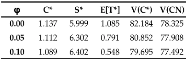
and the increased attractiveness of a new and improved asset cost.

Table 7: Effect of changing the tax credit rate

φ C* S* E[T*] V(C*) V(CN)

0.00 1.137 5.999 1.085 82.184 78.325

0.05 1.112 6.302 0.791 80.852 77.908

0.10 1.089 6.402 0.548 79.695 77.492

Table 7 suggests that an increase in tax credits act as an incentive for asset exchange, which further suggests two other effects. The first effect is the reduction of the net acquisition price. The second effect is the corresponding decrease in the asset salvage value (from the change in the depreciation base). In functional terms, the increase in ϕ corresponds to negative variation in the acquisition price P, which is a similar effect to the one previously discussed in the analysis of the acquisition price.

The tax credit rate ϕ, the tax rate τ , and the depreciation rate δa constitute the tax vector. While variation in ϕ effects the level of the acquisition price and the depreciation base, the change in

τ

is reflected not only in the tax savings value given by C but also in taxation resulting from

(

*

( )

*

)

S C

τ −ϑ⌢

.

The growth of tax rate

τ

suggests an increase in the critical level for asset exchange, and consequently, an increase in the critical period. This results from

the fact that incremental increases in the tax rate also increase the taxes charged to capital gains received from reduction of the net salvage value. In this situation, the new asset becomes less attractive, and maintenance of the current asset is favored by the C

(

1−τ

)

reduction and by the increased contribution of depreciation cost Cδ to the reduction in total costs.

Table 8: Effect of changing the tax rate

ττττ C* S* E[T*] V(C*) V(CN)

0.10 1.030 6.454 0.078 94.807 92.775

0.30 1.137 5.999 1.085 82.184 78.325

0.50 1.386 5.998 4.333 70.033 63.874

Table 8 shows an increase in *

C increase resulting from tax rate

τ

growth. This scenario is an outcome of lower cost flows and lower current values and results from the OMC and net revenue increase.

In the two-factor model, the behavior of *

C with changes in the depreciation rate depends on two effects. The effect of tax savings, defining the depreciation rate as:

(

1

)

a Z a N C C P C δ δ _{δ ϕ} −   = −     , (16)

and the effect of converting this cost into a perpetuity through the opportunity cost: * 1 2 1 2 a a a f C C r r Z Z Z δ α δ δ δ σ         = − − − − − −        . (17)

Table 9 does not indicate any consistent effect of increasing the depreciation rate

δ

a

Table 9: Effect of depreciation rate variation

δδδδa C* S* E[T*] V(C*) V(CN)

0.25 1.011 6.175 0.011 50.734 48.949

0.50 1.137 5.999 1.085 82.184 78.325

0.75 1.078 6.225 0.434 76.531 73.014

As Table 9 shows, when the depreciation rate increases, the critical level oscillates around a reference value. Thus, while increases in the depreciation rate up until 0.5 provokes critical level growth, increases in the depreciation rate above 0.5 causes a reduction in the critical level. In the two-factor model, there are various effects. OMC moves away from its initial value, tax savings are reduced and it modifies the opportunity cost used to discount the net tax depreciation cost.

When δa <0.50 there is an incentive to delay replacement because tax savings prevail due to reduction in the net replacement cost and the potential increase in capital gains. When

δ

a ≥0.50

, the increase in the depreciation rate contributes to the erosion of the asset’s taxable base, which motivates replacement. These considerations of critical level behavior as a function of the depreciation rate can be compared to Dixit and Pindyck (1994). According to these authors, inclusion of depreciation diminishes the investment opportunity of the project. The analogy to the replacement problem is the reduction in the incentive to replace the asset.

6.

Conclusion

This article presented a new methodology for approaching the optimal asset replacement problem in terms of assets with a fixed tax regimen applied to one-cycle cases. It demonstrates how it is possible to evaluate OMC using a two-model factor. This two-model incorporates the flexibility of choosing the appropriate salvage value to make an optimal replacement decision. Thus, one analyzes the

replacement decision in a one-cycle environment where salvage value S is decreasing and follows a GBM.

Thus, a new formula for OMC evaluation has been developed and one do provided some outcomes from numerical simulations applied to the numerical case. Besides, with this different dynamics of salvage value S , one can collect evidence concerning anticipation of the asset replacement decision. This evidence confirms the significant influence of S in the evaluation of OMC. The next step is extending the analysis carried out in this work to a multi-cycle environment.

Appendix A.

This section uses the Method of Characteristics to find a new system of coordinates and reduce the differential equation to its canonical form. This reduction allows the application of the Method of Separation of Variables (Weinberger, 1995). This application will result in a closed solution on which boundary conditions are applied. Following Polyanin (2001), one begins with a general form of a second order partial differential equation:

2

xx xy yy x y

aExc + bExc +cExc +dExc +eExc + fExc=g, (18)

where a b c d e f g, , , , , , are coefficients of the equation classified as parabolic in the cases where b2−ac=0. Thus, it is possible to reduce equation (5) to its canonical form through the introduction of a new system of coordinates

( )

θ η, :

(

, , , ,

)

Exc_θθ =

φ θ η

Exc Exc Exc_{θ η} , (19)

2 2 1 2 C a= σ C , 1 2 C S CS b= σ σ CSρ , e 1 2 2 2 S c= σ S , (20)

from which one obtains the following determinant:

(

)

2 1 2 2 2 2 2

1

4 C S CS

b −ac= σ σ C S ρ − .

Admitting that equation (18) is classified as parabolic, we need to change system coordinates,

(

C S,

)

− >

( )

θ η, , it will be necessary to solve the following equation:

0 S C S C S C σ η η σ + = , where C C η η = ∂ ∂ e S S η η =∂

∂ . The solution is:

S C dS b S dC a C σ σ = = ,

rearranging, one obtains:

S C dS dC S C σ σ = ,

( )

( )

0 S C ln S σ ln C S σ = + ,

from which results:

(

,

)

0 _S C S C S S C σ σ η = = . (21)

For θ, one chooses a function that intercepts the lines of constants, such as:

(

C S,

)

C

θ = . (22)

Differentiating the expressions (21) and (22):

(

)

1 , S C S C C S C S C σ σ σ η σ + = − ,

(

,

)

S C S C S C σ σ η = − ,

(

,

)

1 C C S θ = , θ_S

(

C S,

)

=0, for C C θ θ =∂ ∂ and S S θ θ =∂

∂ . AssumingExc C S

(

,

) ( )

=v θ η, , one calculates:

1 S C S C C S Exc v v C θ σ η σ σ σ + = − ,

S C S Exc C v σ σ η − = , 2 2 2 1 2 2 2 S S C C S S CC C C S S Exc v v v C C θθ σ θη σ ηη σ σ σ σ σ + σ + = − + , 2 1 S C SS Exc v C ηη σ σ = , 2 1 1 S S C C S CS C S Exc v v C C θη ηη σ σ σ σ σ σ + = − .

Just before making the substitution in equation (5) we simplify the following expression:

(

)

2

2 2 2 2

1 1 1

2ExcCCσCC +ExcCSσ σC SCS+2ExcSSσSS =2 ExcCσCC+ExcSσSS . (23) Substituting the new coordinate

ξ

and ηin the last equation:

2 2 1 2 C C S f S C C v_θθ r v α σ v_η v_θ σ θ α η α θ σ   = − −  −   . (24)

To find a general solution, Abell and Braselton (1997) suggest the transformation q=θ and r =η, producing the function v

( ) ( )

θ η, =v q r, . The solution will result from the product of two functions, each one depending only on one independent variable. This process is typically called the Method of

Separation of Variables (Weinberger, 1995) and serves to convert a partial differential equation into an ordinary differential equation. Thus, considering:

' dQ Q dq = e 'R dR dr = , and

( )

,

( ) ( )

v q r =Q q R r .

Differentiating v

( )

. , one obtains:

' q v_θ =v =Q R, ' r v_η = =v QR , '' qq v_θθ =v =Q R.

Applying these expressions to (24), one transformation produces:

2 '' ' ' _f 0 q Q RΠ +ξξ qQ RΠ +ξ rQR Π −η r QR = . (25) with 2 1 2 C ξξ σ Π = , C ξ α Π = , C S S C η α α σ σ Π = − ,

where rf corresponds to the risk-free rate of interest. Splitting equation (25) into

two separate equations, one a function of R and another a function of Q .

2 2 ' '' ' f f a r R q Q qQ r Q k R Q ξξ ξ η Π + Π − −Π = = − ,

where ka is a constant. Thus, the previous expression allows us to obtain the

following differential equations:

2 ' 0 a f k R−r R Π =η , (26) and

(

)

2 2 '' ' _{f a} 0 q Q Π +ξξ qQ Π −ξ Q r −k = (27)

To find the expression for R, one manipulates (26): 2 a k dR dr R =Πη r ,

( )

2

( )

1 a k ln R = _η ln r +k Π ,

( )

( )

ka2 r R r =k r Πη

where kr is a constant. Proceeding in similar way for Q, one verifies the

presence of a Cauchi-Euler equation for which the following general solution exists:

( )

1 2 1 2 Q q =k qϖ +k qϖ , (28) where

( )

(

)

(

)

(

(

)

)

(

)

2 _{2 * 2 2} * * 2 2 2 2 2 2 2 1,2 2 2 2 8 8 2 1 16 2 2 2 a f C a f C C C C a f a f a f C a f a f C C k r k r k r k r k r k r k r α σ α α σ σ σ ϖ σ   − −   − _± − − + + − −_ − − − −     = . (29)

Consequently, the expression v q r

( )

, =Q q R r

( ) ( )

takes the following form:

( )

( ) ( )

(

)

2 1 2 1 2 , a k r v q r =Q q R r = k qϖ +k qϖ k rΠη ,

( )

2 2 1 2 1 2 , a a S S k k r r v q r k k q rϖ α k k q rϖ α     = +     ,

( )

2 2 1 2 1 2 , a a S S k k r r v q r =k k q rϖ α +k k q rϖ α ,

( )

2 2 1 2 , a a S S k k A B v q r =k q rϖ α +k q rϖ α . (30)

Replacing q and r by the corresponding terms in C and S, one achieves the general solution (6).

References

Abell, M. e Braselton, J. (1997). Differential Equations with Mathematica. London: Academic Press.

Adkins, R. (2005). Real options analysis of capital equipment replacement under

revenue uncertainty. Working paper, 106. University of Stanford.

Bernstein, P. e Damodaran, A. (1998). Investment Management. New York: John Wiley & Sons.

Brach, M. (2002). Real Options in Practice. New Jersey: Wiley, John & Sons, Incorporated.

Dixit, A. (1989). Entry and exit decisions under uncertainty. Journal of Political

Economy, 97, 620-38.

Dixit, A. e Pindyck, R. (1994). Investment under uncertainty. Princeton University

Press.

Dobbs, I. (2002). Replacement investment: Optimal economic life under uncertainty. Working paper. University of Newcastle.

Keles, P., e Hartman, J. (2004). Case study: Bus fleet replacement. The Engineering

Economist, 49 (3), 253–278.

Hull, J. (1993). Options, Futures and Other Derivatives. New Jersey: Prentice Hall. Margrabe, William (1978). The value of an option to exchange one asset for

another. Journal of Finance, 33 (1), 177-186.

Mauer, D. e Ott, S. (1995). Investment under Uncertainty: The Case of Replacement Investment Decisions. Journal of Financial and Quantitative

Analysis, 30, 581-605.

Merton, R. (1973). Theory of Rational Option Pricing. Bell Journal of Economics and

Mun, J. (2003). Options Analysis Course: Business Cases and Software Applications. New Jersey: Wiley, John & Sons, Incorporated.

Polyanin, A. (2001). Handbook of Linear Partial Differential Equations for Engineers

and Scientists. London: CRC Press.

Rust, J. (1985). Stationary Equilibrium in a Market for Durable Assets.

Econometrica, 53 (4), 783-805.

Ye, M.H. (1990). Optimal Replacement Policy with Stochastic Maintenance and Operation Costs. European Journal of Operational Research, 44, 84-94.

Weinberger, H. (1995). A First Course in Partial Differential Equations With Complex