MODELING THE IMPACT OF GOLD MINING ON ECOSYSTEM SERVICESIN GHANA´S SOUTHERN WATER BASINS
MODELING THE IMPACT OF GOLD MINING ON ECOSYSTEM SERVICES IN GHANA´S SOUTHERN WATER BASINS
Thesis supervised by
Pedro da Costa Brito Cabral, PhD
NOVA Information Management School, Universidade Nova de Lisboa, Lisboa, Portugal.
Judith Verstegen, Jun. Prof. Dr.
Institute for Geoinformatics (IFGI),
Westfälische Wilhelms-Universität, Münster, Germany.
Carlos Granell Canut, PhD
Institute of New Imaging Technologies (INIT) Universitat Jaume I, Castellón, Spain.
Thesis submitted by
Jonas Moritz Meyer To:
Universidade Nova de Lisboa, NOVA – Information Managemant School Lisbon, Portugal
Westfälische Wilhelms-Universität Münster, Institute for Geoinformatics (ifgi)
Münster, Germany
Universitat Jaume I, Dept. Lenguajes y Sistemas Informaticos Castellón, Spain
Declaration
I, Jonas Moritz Meyer, declare this Master thesis entitled “MODELING THE
IMPACT OF GOLD MINING ON ECOSYSTEM SERVICES IN GHANA´S SOUTHERN WATER BASINS” was composed independently as a
requirement for the Master of Science in Geospatial Technologies. This thesis is based on my work and under the guidance of my supervisors.
It contains no material that has been submitted previously, in whole or in part, for the award of any other academic degree or diploma. Except where otherwise indicated, this thesis is my own work.
February 2019 Lisboa, Portugal
Abstract
All natural resources are more or less limited and they can be overused and destroyed. While nature degradation occurs, political decisions are often short-sighted and profit-oriented, the importance of ecosystems is often unknown or less important than other interests for the decisionmaker. In this work, we apply GIS technics and InVEST models within a gold mining area in the southern water basins in Ghana. The aim was to identify the impact of mining activities on ecosystem services. The research was done with freely available datasets. It was possible to model and map water and soil pollution and to identify differences between regions were gold mining is taking place and regions without it. Gold mining was identified as a threat to the quality of the habitat and the water and soil quality regulation ecosystem services. This work may contribute to mitigate the negative effects of gold mining activities.
KEYWORDS
Ecosystem services Gold mining
Habitat quality InVEST
Land cover analysis Water pollution
ACRONYMS
CGIAR-CSI – Consultative Group for International Agricultural Research CICES - Common International Classification of Ecosystem Services DEM – Digital Elevation Model
DLR – Deutsches Zentrum für Luft- und Raumfahrt ES – Ecosystem Services
ESA – European Space Agency GDP - Gross Domestic Product
GIS – Geographic Information System GNI – Gross National Income
HQ – Habitat Quality model
InVEST – Integrated Valuation of Ecosystem Services and Tradeoffs ISRIC – International Soil Reference and Information Centre
JRC/EC – Joint Research Centre / European Commission LC – Land Cover
LULC – Land Use Land Cover
NASA – North American Space Agency
NDR – Nutrients Retention and Delivery model OSM – OpenStreetMap
SRMT – Shuttle Radar Topography Mission USD – United States Dollar
INDEX OF TEXT
1. Introduction ... 1
2. Literature review ... 3
2.1 Ecosystem Services ... 3
2.2 Reasons for ES degradation ... 6
2.3 Water and Soil pollution ... 7
3. Study area ... 10
3.1 The study Area inside Ghana's southern water basins. ... 10
3.2 Gold Mining in Ghana ... 12
4. Methodology ... 15
4.1 Data and pre-processing ... 15
4.2 Methods ... 25
4.2.1 Invest ... 25
4.2.2 Estimation of Copper and Zink at the Ankobra ... 26
4.2.3 Estimation of Nitrogen (N) and Phosphorus (P) ... 29
4.2.4 Estimation of Mercury (Hg) ... 32
4.2.5 Habitat quality ... 35
5. Results ... 40
5.1. Copper and Zinc ... 40
5.2. Nitrogen and Phosphorus ... 43
5.3 Mercury ... 46
5.4 Habitat Quality ... 47
5.5 Comparison of model results inside and outside gold mine areas ... 50
6. Discussion ... 52
6.1 Contributions ... 52
6.2 Limitations ... 52
6.3 Future work ... 53
References... 57
Annexes ... 60
Annex A: Create the Study area layer ... 60
Annex B: Create River area and Gold mining LC layer ... 61
Annex C: Create copper content tables for every LULC class ... 62
Annex D: Create Input layers for the InVEST NDR model ... 63
Annex E: Seasonal mercury delivery layer ... 64
Annex F: Threats to habitat tables (Terrado, M., Acuña, V., Mandle, L., Sabater, S., Ziv, G., & Chaplin-Kramer, B. , 2015)... 65
INDEX OF FIGURES
Figure 1 Study area ... 11
Figure 2 Small scale gold mining spots 1 ... 17
Figure 3 Small scale gold mining spots 1 ... 21
Figure 4 Small scale gold mining spots 2 ... 21
Figure 5 Large scale gold mine ... 22
Figure 6 Industrial quarter ... 23
Figure 7 Small scale gold mining spots and river systems ... 24
Figure 8 Diagram of copper and zinc estimation within the Ankobra river system ... 27
Figure 9 Study area at the Ankobra river ... 28
Figure 10 NDR inside and outside mining area ... 32
Figure 11 Diagram for mercury delivery and retention model ... 33
Figure 12 Diagram of habitat quality estimation ... 36
Figure 13 Threat map ... 37
Figure 14 Soil zinc content ... 42
Figure 15 Soil copper content ... 42
Figure 16 NDR Nitrogen (Annual) ... 44
Figure 17 NDR Phosphorus (Annual) ... 45
Figure 18 Mercury delivery (Annual) ... 46
Figure 19 Result of the Habitat Quality Model ... 47
Figure 20 Habitat quality within and without the mining area ... 48
INDEX OF TABLES
Table 1 Pressures and indicators for ecosystem condition assessment (HAINES-YOUNG &
Potschin-Young, 2017) ... 4
Table 2 CICES classification (HAINES-YOUNG & Potschin-Young, 2017) ... 5
Table 3 Pressures ES Value and grade of degradation (Sutton et al. 2016) ... 7
Table 4 Climatic characteristics of Ghana ... 11
Table 5 Datasets used ... 15
Table 6 Nutrients and phosphorus load per land cover class (adapted from Leh et al, 2013) ... 30
Table 7 Values of the NDR “Biotable” (adapted from Leh et al., 2013) ... 31
Table 8 Sensitivity of landcover to threats ... 39
Table 9 Threat table ... 39
Table 10 Zinc and Copper content in mg/100kg ... 40
Table 11 Differences of heavy metals in mg/100kg ... 41
1
1. Introduction
The natural environment is featured by species and physical processes which are all involved in more or less complex interactions. These species, processes, and interactions on a specific area can be described as a
particular system, the ecosystem. Every ecosystem is embedded in and interacting with circulating flows of substances and the climate. Many ecosystems of the world are nowadays under pressure by more and more intense and overexploiting anthropogenic land use and related pollution and other biophysical changes like global warming.
In developing countries such as Ghana, where poverty is a severe problem for many inhabitants it should be understandable that the protection of the natural environment is not their primary concern while policy making. When the protection of ecosystems has to compete with economic development, it has to get in line most of the times (Turpie, Forsythe, Knowles, Blignaut, & Letley, 2017a; Turpie, Heydenrych, & Stephen J. Lamberth, 2003).
But there is no doubt that the unsustainable use of natural resources is not just resulting in directly occurring adverse effects like water or air pollution, but also in long term effects like soil degradation. These adverse effects are finally resulting in losses for the national economy and, nevertheless decreasing people’s livelihood.
Labeled with the term Ecosystem Services (ES) researches are done where the measurement of benefits for people provided by ecosystems is the primary research object. In this paradigm, ecosystems are viewed from an economic perspective. Unsustainable use of natural resources and pollution are degrading the valuable outcome of ecosystems which is decreasing income and causing costs (Costanza, Groot, et al., 2014).
Against this background, this master thesis reports about a biophysical assessment of the spatially explicit extent of land degradation through pollution in Ghana´s gold mining region implemented by InVEST models (InVEST, n.d.) and Geographical Information Systems (GIS).
2
The aim was to identify the impact of mining activities on the environment and, therefore, on the habitat quality and to ascertain the damage of the ecosystem.
Habitat means the living environment of any species and is assembled by several conditions that allow life. The habitat quality depends on the availability of several different resources and is decreasing through anthropogenic land use and pollution.
Related research questions developed to reach this aim were:
• Is there a difference in soil pollution inside and outside the gold mine areas?
• Is there a difference in nutrient retention by the landscape inside and outside the gold mine areas?
• What is the habitat quality inside and outside the gold mine areas?
Based on these research questions, the following hypotheses were developed:
• Gold mining can be considered a threat to soil and water quality. • Gold mining can be considered as a threat to habitat quality, and
this is possible to illustrate with InVEST.
To approach the answers to the research questions and report about the impact of gold mining on ecosystem services, it is first discussed the framework in which this study is embedded, after that it is presented the methodology and the results of the practical research that was done.
3
2. Literature review
2.1 Ecosystem Services
Humans health, livelihoods, and survival are depending on a range of services provided by ecosystems, the ecosystem services (ES) (Tallis & Polasky, 2011). ES is a growing interest for researchers and policymakers around the world (de Groot et al., 2012). The specialty of the ES paradigm, and therefore its importance for science, is the integrative relationship between humans and their natural environment, that allow a pragmatic view on the impact of ecosystem degradation on living quality.
For proper sustainable protection of the ecosystems and their services, the usage of their goods and benefits need to be balanced between people and economy on the one hand, and the assumed biotic equilibrium on the other hand. This understanding is crucial for building a sustainable and desirable future society (Costanza, de Groot, et al., 2014).
Besides contributing to people's well-being, ecosystems are also a
significant contributor to the economy. The total monetary value of ES is around 33 trillion US Dollar per year and exceeds the overall global gross domestic product(Costanza et al., 1997). This is why the idea that people have to decide between nature and the economy is false. Instead, it should be considered how to manage natural and human-made capital efficiently and sustainable.
The primary goal of any ES approach should be to clarify the direct and indirect benefit of natural capital for the people (Potschin & Haines-young, 2011). On base of researches on ES, it is than possible to value ecosystems and their protection. Approaches for valuation and mapping of ES can inform policy decision maker about the role of the natural capital within regional planning and development, conservation and restoration of landscapes and their delivery benefits to the people (Turpie, Forsythe, Knowles, Blignaut, & Letley, 2017b).
4
ES assessments are generally based on the quantity of the service, and the spatial distribution of ecosystems as the basic input parameters (Benjamin Burkhard & Maes, 2017a). For more accurate results it is necessary to assess also the condition of the system, which allows viewing the quality of the service. The amount of timber provided by a forest, as example, is not only depending on the extent of the forest, but also the composition of the trees and their age.
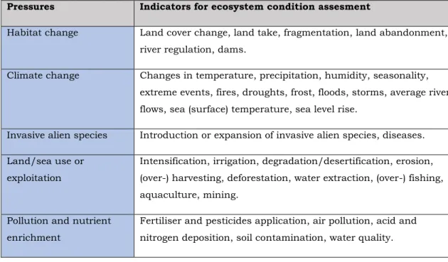
The main anthropogenic effects which pressure the ecosystem are habitat change, climate change, invasive species, land management, and pollution and nutrient enrichment (Table 1).
Table 1 Pressures and indicators for ecosystem condition assessment (HAINES-YOUNG & Potschin-Young, 2017)
Pressures Indicators for ecosystem condition assesment
Habitat change Land cover change, land take, fragmentation, land abandonment, river regulation, dams.
Climate change Changes in temperature, precipitation, humidity, seasonality, extreme events, fires, droughts, frost, floods, storms, average river flows, sea (surface) temperature, sea level rise.
Invasive alien species Introduction or expansion of invasive alien species, diseases. Land/sea use or
exploitation
Intensification, irrigation, degradation/desertification, erosion, (over-) harvesting, deforestation, water extraction, (over-) fishing, aquaculture, mining.
Pollution and nutrient enrichment
Fertiliser and pesticides application, air pollution, acid and nitrogen deposition, soil contamination, water quality.
While the threats to the ecosystems are plenty and diverse their services are also. To overcome problems in the exchange of scientists regarding
researches on the interactions between humans and ecosystems, standards and classifications are helpful.
One standard is the Common International Classification of Ecosystem Services (CICES) (HAINES-YOUNG & Potschin-Young, 2017).
5
CICES classifies the final services that interface between ecosystems and society. They are split into three main categories:
• Provisioning services are all material and energetic outputs of an ecosystem from which goods are produced.
• Regulating services are all the positive physical and chemical influences of an ecosystem which are helping to maintain the people's natural environment.
• Cultural services are all features of an ecosystem that are
contributing to the mental or intellectual well-being of the society.
Table 2 CICES classification (HAINES-YOUNG & Potschin-Young, 2017)
An essential aspect of the CICES categorization is the differentiation of services and benefits. While service is a direct output of the ecosystem, the benefit is the final good used by the society which arises by human
processing of the service. The importance of this differentiation is the identification of services independent from the natural goods derived by an ecosystem. Every service could lead to more than one benefit at the same time (Benjamin Burkhard & Maes, 2017b; Levrel, Cabral, Feger, Chambolle, & Basque, 2017).
6
2.2 Reasons for ES degradation
Ecosystems and their services are mainly degraded through anthropogenic land use and pollution. To stop the extent of degradation and restore the ecosystems is important, especially inside the tropics where the climate change is (and probably will be) causing climatic extreme events and unpredictability of rainfall patterns (Kubiszewski, Costanza, Anderson, & Sutton, 2017).
Within western Africa ecosystems are under pressure due to human’s expansive utilization and the overexploitation of natural resources, on a local or nationwide scale and due to threats like invasive species and
climate change on a global scale (Leh, Matlock, Cummings, & Nalley, 2013). As the main driver of ecosystem degradation, it was identified land cover change. Probably due to the lack of suitable data, just a few researches on ES based on land cover change in Africa were done until now. Although that, especially this continent is featured by strong and ongoing changes in land use and economic and demographical dynamics. For this reason, such analyses are important for policy decision making (Niquisse & Cabral, 2017; Wangai, Burkhard, & Müller, 2016).
In Ghana, the main driver of land cover change is agricultural expansion. On the one hand, a growing population needs more food, on the other hand, crop plants like, as for example, cocoa, are growing for the world market because the economy is still mainly based on the production of raw materials (Leh et al., 2013).
For the identification of land cover change in huge areas, the most appropriate method is remote sensing. Coulter et al. (2016) performed a land cover change analysis with Landsat 7 ETM+ imagery for the provinces Ashanti, Central, Eastern and Greater Accra which are all (at least partly) located within the study area of this thesis as it can be viewed in Figure 1. From all the land surface within the four surveys provinces 26 percent exhibit land cover changes. Most of those changes (62%) were agriculture expansion, but also 2,2 percent were an expansion of mining area. In total,
7
the mining area increased from 0,48 km² in 2000 to 2,89 km² in 2010 which is a rise of 602 percent (Coulter et al., 2016b).
Huge expansion of mining area was also reported from the Ankobra water basin, where the area increased from 4,3 km² in 1991 to 137 km² in 2016. The water landcover class increased as well due to the mining water inside the pits of the abandoned mines (Obodai, Adjei, Odai, & Lumor, 2019). Although protection and conservation should be an important interest for the population and their policymakers, generally other economic interests have got a higher priority (Turpie et al., 2017b). To overcome this problem, it could be important to communicate the monetary value of ecosystems based on their services. Kubiszewski et al. (2017) were calculating the monetary value of ES for every country in the world, both actual and potential. Based on this approach they estimate the rate of degradation as the gap between the potential and the actual value. In table 4 their results for the monetary value of ES are presented for Ghana and as an example for comparison, Portugal, Germany, and Spain, as well as for the whole world together.
Table 3 Pressures ES Value and grade of degradation (Sutton et al. 2016)
Name ESV Potential (Mill. USD/Y) ESV Degraded (Mill. USD/Y) % Degradation
Ghana 105370,42 83921,87 20,4
Portugal 39854,11 30351,24 23,8
Germany 179034,86 174173,82 2,7
Spain 225871,32 174941,01 22,5
World 68782784,67 62462358,24 9,2
2.3 Water and Soil pollution
The understanding and research of the local water cycle is vital for the estimation of the pollution caused by substances within the surface.
8
The land surface is an essential component of the water cycle because it is determining the flow direction and the amount of water which seeps into the soil and finally into the groundwater (Eduful & Shively, 2015).
Humans use the land in multiple ways, which introduces diverse and complex changes on land use and the hydrographic system. Anthropogenic impacts are either a change of the water flow in shape and size or
alterations of the water quality through pollution. While anthropogenic activities are constantly polluting the environment, the surface runoff is depending on the climate and is an inconstantly and a seasonal
phenomenon (Asare-Ansa et al., 2014).
The estimation of the extent of waste treatment on the water quality, caused by substances in a given area, is usually done with models for sediment transport. This estimation is achieved by combining soil maps with calculations for the capacity of the vegetation and the river systems to
retain nutrients and sediments from agriculture. More elaborate studies use more hydrological indicators, topographic data, and information about the specific land use, like the different agricultural processes and their input into the soil (Crossman et al., 2013).
While most of the waste-water will flow through the river system into the ocean, some amount of soil pollution (depending on the retention efficiency) will stay within the land surface where it occurs.
For the modeling of the available water yield of an area, river basins are often used as the spatial unit. As the input parameters information about the precipitation and evapotranspiration, as well as maps for soil and land-use types are land-used. The models range from simple water balance
estimations (input-output = consumable water) to complex hydrological models using data for the daily precipitation, stream gauge, water storage capacity and water extraction for an improved and partially explicit water flow model (Crossman et al., 2013).
Soil pollution is a result of anthropogenic activities such as industrial production, the traffic or the use of crop fertilizer and pesticides.
9
important source of soil pollution and therefore as well of soil degradation (Sun, Xie, Wang, Hu, & Cheng, 2018a).
The degradation caused by mining activities includes the destroying of the surface within the mining area, the production of often toxic waste as side products (tailings or drainage) and the emission of dust, enriched with heavy metals to the atmosphere. The most problematic type of mining, even more, when it is illegal, is small-scale mining. These mines are a serious threat to the health and the security of the population that lives close to them (Sun, Xie, Wang, Hu, & Cheng, 2018b).
In Ghana widespread land cover change and land degradation as a result of mining area expansion is reported. Consequences are changing livelihoods and land use conflicts (Schueler, Kuemmerle, & Schröder, 2011).
10
3. Study area
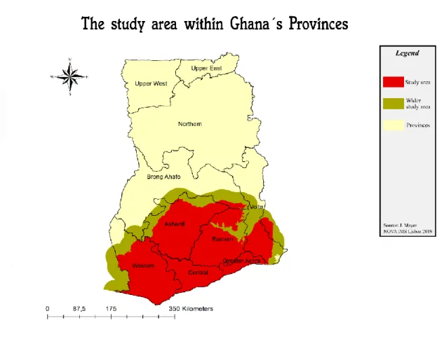
3.1 The study Area inside Ghana's southern water basins.
For a study of substances flow, it is suitable to use water basins as the borders of the study area because they cover all possible flow directions within their area. Ghana´s southern water basins (Figure 1) are chosen as the study area in this research because:
• Within is located one of the most important gold mining areas of the
world.
• It has the highest population density in Ghana, containing the two major cities Kumasi and Accra.
• Its landscapes are widely shaped by humans.
Another important fact that influenced the study area election, is that Ghana is facing a relatively huge grow in population and in the economy rate. The population in Ghana is in continuous growth, increasing from 5 million in 1950 to 19 million in 2000, 25 million in 2010 and 28,2 million in 2016 (Coulter et al., 2016b; World Bank, n.d.). According to the United Nations Population Division, the population will continue growing up to 50 million in 2050. An increase in urbanization accompanies this increment in the population. The number of inhabitants that are living in cities increased from 15% in 1950 to 52% in 2010, and it is expected to be 75% in 2050 (Coulter et al., 2016).
For the Gross Domestic Product (GDP) the World bank was calculating 42690 million US-Dollar, which is 1513 USD per capita. The Gross National Income (GNI) was calculated to be 41299 million USD, which is 1380 USD calculated with the World banks Atlas method (World Bank, n.d.).
11 Figure 1 Study area
Regarding the weather, Ghana is a tropical country when following the Köppen classification. The tropics are characterized by high temperatures (generally over 18ºC), an absence of thermal seasons and plentiful
precipitation distributed in rainy and dry seasons. Moreover, the
temperature difference between day and night is more significant than that between the warmest and the coldest month.
A specific lookup on the main climatic characteristics of Ghana, extracted from the weatherbase.com and are shown in table 4 (Weatherbase, n.d.).
12
Table 4. shows values for the average temperature (in Celsius) and the average precipitation (in millimeter per square meter) in Ghana, both for one year (Annual) and for every month. The colors represent different values, high values (red), medium values (orange) and low values (green). It represents, on the one hand, that the temperature is relatively high the whole year and does not have big variations during the seasons. On the other hand, the precipitation shows two seasons, a rain-season from April to October and a dry-season from November to March. This regularity is interrupted in August, where the precipitation is lower than in July and September.
This climate influences the rivers resulting in reduced or even missing water flow occurring during the dry season. Lower reaches of the Pra River generally flow the whole year whereas the upper Pra River, the Mamang River, and the other tributary streams flow seasonally during raining periods (Attiogbe & Nkansah, 2017).
3.2 Gold Mining in Ghana
Gold is a particular resource because of its function as money and its very high price. During the world financial crisis that started in 2008, capital investments were secured by navigation into a so-called, safe harbour. One of these harbours is gold because of its high value for being a rare metal. Ghana seems to face a resource curse dilemma: The increasing amount of exported minerals is increasing the countries overall income, but as well the dependency on these minerals, while other economic sectors lack in their development Schueler, Kuemmerle, & Schröder, 2011).
According to the Ghana Chamber of Mines, Ghana has a long history of mining. More than half of the foreign direct investment is produced by the mining sector which makes an essential contribution to the gross domestic product (GDP) and creates a large number of jobs. The exploiting minerals in Ghana include gold, manganese, limestone, and diamonds, among others. In particular gold is the most important good that
13
contributes more than 95 percent of the country´s total mineral benefit (Attiogbe & Nkansah, 2017).
For a brief overview, Ghana exported gold for around 4428 Million US Dollar in 2016 (World Bank, n.d.). The average gold price in the same year was 39775 US Dollar per kg (GOLD). This means Ghana exported a total of 111.326 kg of gold in 2016.
To obtain these huge amounts of gold, large land areas are affected. Hausermann et al. (2018) conducted a remote sensing analysis in Ghana's gold mining region, where they found out that vast areas were transformed into gold mining land between 2008 and 2013. The total extent of gold mining spots inside their study area increased from 0,35 km² into 8 km². The size of the so-called mining water, which is stagnant water inside the abandoned pits of former mining spots, was increasing from 0,02 km² to 2 km². Nineteen roads that are leading to the mining sites expanded from together 36,3 km to 88,5 km (Hausermann et al, 2018).
Many effects of the land cover changes and its related impacts are not occurring immediately but are visible after some years. Therefore, in-depth knowledge of the place is needed to understand the uncertain long-term outcome of gold mining. The local population reported about long-term severe consequences of the mining expansion, such as diseases through polluted water bodies or food insecurity (Hausermann et al, 2018). In Ghana all land that is accounted as areas for mineral exploration is about 12 percent of the whole country. Gold is nowadays (since the start of a gold rush in the 1980s) the main mineral that is extracted. It can be found particularly within reef formations and valleys and on the riverbanks Schueler, Kuemmerle, & Schröder, 2011).
There are two types of extracting gold which differs in their procedure and their caused pollution: Large-scale mining companies with industrialized processes and small-scale miners that skim the soil at the riverbanks with their hand to sell the gained gold on local markets (Schueler, Kuemmerle, & Schröder, 2011). Small-scale gold extraction is polluting water bodies, soils and the air with arsenic, mercury and sulfur contaminations which lead to
14
degraded environments containing acid rains and impacts on human health (Ansa et al., 2014).
In Ghana, gold mining is mainly located on the river Pra which flows
through the Western, Eastern and Ashanti regions. The water bodies inside this area contain high values of Hg (Mercury) and toxic heavy metals as, cadmium, copper, zinc, and lead (Ansa et al., 2014).
15
4. Methodology
4.1 Data and pre-processing
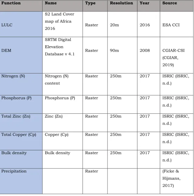
For the performance of this research, it was possible to apply several actual datasets with high-resolution. The table below shows which datasets were used, their resolution and source.
Table 5 Datasets used
Function Name Type Resolution Year Source
LULC
S2 Land Cover map of Africa
2016 Raster 20m 2016 ESA CCI
DEM
SRTM Digital Elevation
Database v 4.1 Raster 90m 2008 CGIAR-CSI (CGIAR, 2019) Nitrogen (N) Nitrogen (N)
content
Raster 250m 2017 ISRIC (ISRIC, n.d.)
Phosphorus (P) Phosphorus (P) Raster 250m 2017 ISRIC (ISRIC, n.d.)
Total Zinc (Zn) Zinc (Zn) Raster 250m 2017 ISRIC (ISRIC, n.d.)
Total Copper (Cp) Copper (Cp) Raster 250m 2017 ISRIC (ISRIC, n.d.)
Bulk density Bulk density Raster 250m 2017 ISRIC (ISRIC, n.d.)
Precipitation Raster (Ficke &
Hijmans, 2017)
16 OSM Vector Layer OSM
DatasetGhana Vector 2018 Geofabrik (“GeoFabrik,” n.d.) Admin. Boundaries
HUM Data Vector 2016 Hum Data
(Humdata, 2019)
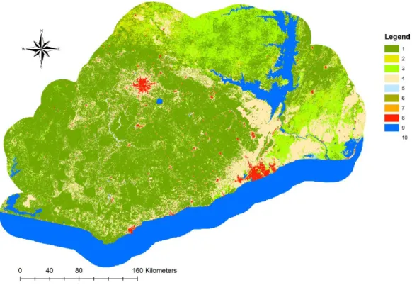
As the land cover map (LULC), the S2 prototype Land Cover 20m map of Africa 2016 was used (Figure 2). It is based on one-year long observations done by the Sentinel- 2A satellite-based system. Its creation process realized by the European Space Agency (ESA) includes image analysis and classification. Cloud-free remote sensing imagery was classified with Random Forest and Machine Learning algorithms and then overlaid to predict the most suitable landcover class for every pixel.
The identification of open water and urban areas was supported by the use of external datasets, the Global Surface Water product and the Global Human Settlement Layer from JRC/EC, as well as the Global Urban Footprint from DLR.
Landcover was classified into ten classes: 1. Trees cover areas; 2. Shrubs cover areas; 3. Grassland; 4. Cropland; 5. Vegetation aquatic or regularly flooded; 6. Lichen and mosses / sparse vegetation; 7. Bare areas; 8. Built-up areas; 9. Snow and ice and 10. Open water (ESA, 2019).
17
Figure 2 Small scale gold mining spots 1
The Digital elevation model (DEM) was extracted from the Shuttle Radar Topography Mission (SRTM) Digital Elevation Database v.4.1 which is freely available on the internet. It was processed by NASA and USGS and then pre-processed by the Consultative Group for International Agricultural Research (CGIAR, 2019). The database is covering the United States in 1 arc-seconds (30m at the equator) and the rest of the world in 3 arc-seconds. In its original release, SRTM data contained regions of no-data, specifically over water bodies. Therefore, the pre-processing included several steps to provide a seamless and complete elevational surface for the whole globe (CGIAR-CSI).
Vector layers for locations and infrastructure were extracted from
OpenStreetMap (OSM)(OSM, 2016). OpenStreetMap is an open source world map that was created and is edited by a vast non-profit oriented
community. Although it is possible to download geodata directly from the OSM homepage, this data is hard to use because of the non-standard data format and a missing arrangement by geodata type. For this reason, it is
18
recommended to get OSM data from the company Geofrabrik (“GeoFabrik,” n.d.), that offers cost-free downloads of national and province scale based extractions of the OSM database. These datasets are arranged by type into layers and saved as shapefiles.
The International Soil Reference and Information Center (ISRIC), offers the Soil Metadata Catalogue which contains multiple, high-resolution datasets, especially for Africa. The datasets represent soil properties like the texture, the root zone depth or the pH value of the water content; and soil
components like the sand or iron content. The ISRIC datasets used in this research are (ISRIC, n.d.):
• Total nitrogen (N) in g/kg of the fine earth fraction measured in 0-20 cm
• Total extractable Phosphorus (P) in mg/100kg of the soil fine earth fraction measured in 0-30 cm depth.
• Extractable Zinc (Zn) content in mg/100kg of the soil fine earth fraction measured in 0-30 cm depth.
• Extractable sodium Copper (Cu) of the soil fine earth fraction in mg/100kg of the soil fine earth fraction measured in 0-30 cm depth.
• Bulk density (Bd) of the soil fine earth in kg/m3, measured at six standard depths.
The average precipitation was calculated based on the WorldClim 2.0 global climate layers for monthly average precipitation in mm.
For assessing the amount of pollution that is secreted by gold mining and its influence on the habitat quality, the input data was pre-processed by using ArcMap GIS and Excel. After that, the InVEST models NDR, and habitat quality were conducted. In the following section the methodology is explained in detail:
19 1. Preparation of work environment
The first step of the practical work was to download the datasets and to
install the software.
The work was performed with ArcMap v. 10.5.1 from ESRI, Redlands as GIS, Excel from Microsoft, Redmond for table-based calculations, Google Earth Pro from Google, Mountain View for data extraction and accuracy assessment, InVest from the natural capital project at Stanford University for model processing and Inkscape v. 0.92 for Graphics.
Main parts of the data processing were done with the GIS ArcMap and its Modelbuilder. ModelBuilder is an application within ArcMap that allows arranging desired geoprocessing tools step by step, one after the other. The GIS work environment was created with model builder. Due to the huge amount of data, the created folder structure is cleaned by deleting not useful files.
2. Compilation and cutting to size of the input data
The study area that is the southern water basins of Ghana was extracted from the water basins shapefile with the tool Select by attribute. To respect the influence of the surrounding landscapes on environmental processes, the bordering regions within 30 km were included in the study area by using Buffer and Merge. Besides, to get a more suitable shape for the study area´s shapefile, some adjacent parts that were extracted from a layer with the administrative boundaries of Ghana (Humdata, 2019), were added.
The single merged parts are assembled into one part with the tool Dissolve. To get the value for the output shapefiles extent in km², the input tables fields, “Shape_Area” were aggregated. This shapefile represented the study area plus its surroundings and used to cut out the other datasets with the tool Clip. When Clip was used to cut a portion of a raster dataset, the input dataset was always determining the clipping geometry, and the extent maintained to secure that the single output files had the same shape.
20
From the OSM layers, only some of the data was needed and therefore extracted with Select. Out of the “roads” layer, just the “primary,”
“secondary,” “tertiary” and “residential” class were chosen just to consider streets with relevant traffic volume. From the “places” layer, “city,”
“suburbs” and “towns” were selected to get the locations of the main
settlements. From the points of interest layer, the points that are classified by the following names were selected to identify important tourism sites: “attraction,” “camp site,” “hostel,” “hotel,” “motel,” “tourist info”. After clipping all of the datasets, they were projected by the use of Project Raster to the same coordinate system suitable for the study area: WGS 1984 UTM Zone 30N.
All raster datasets were overlaid with the same foursquare raster to secure that they are overlaying before being exported from ArcMap. The overlay of the spatial input files is a requirement of the InVEST models. Thus, a new raster was created by the tool Create constant raster with the LULC as extent and 0 as the constant value. For unifying layers, Mosaic to new
raster was used.
3. Primary-data preparation
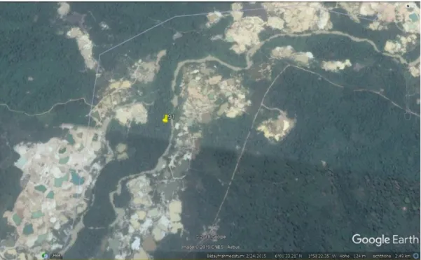
The location of mines and industrial sites was obtained from interpreting remote sensing imagery provided by Google Earth Pro (Figure 2-5).
Within a suitable resolution, it is possible to see the mining spots. They are clearly to identify due to the absence of vegetation and dug over soil with often water-filled pits. Conversely, the surroundings are covered by forest. Nearly all of the small-scale mining sites are located close to rivers whose water is used to wash out the gold from the soil by the use of toxic
substances like Mercury.
Vast parts of the rivers Ankobra and Tano are covered by mining spots,
where most of the fields are, probably, already abandoned. The identified mining spots areas were marked within Google Earth.
Tiny areas were not pointed out and huge mining areas were marked multiple times, following the river flow every 5 kms.
21
The following images (Figures 3 and 4) show two mining sites identified locations where the marker represents the location of a point inside the point-layer “Goldspots”.
Figure 3 Small scale gold mining spots 1
22
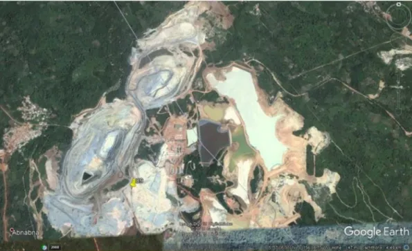
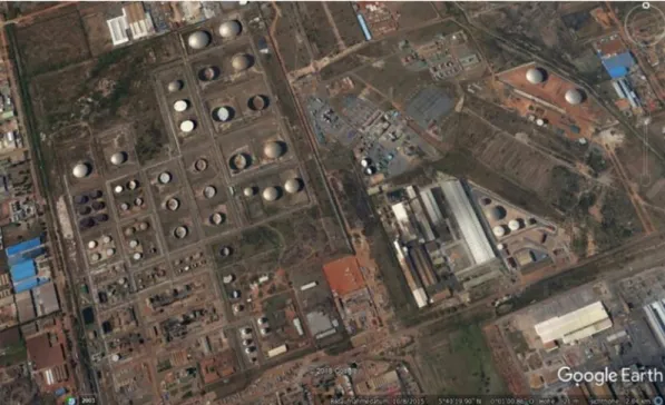
Although gold is extracted in Ghana in both, small and big scale mining, around 96% of it is extracted in big scale mines that are managed by big mining companies. These large-scale gold mines are located on the main gold veins, that are not always close to rivers. For their identification in Google Earth, it was useful to know beforehand where gold veins are located and what their shape and structure are. The following images (Figures 5 and 6) show two mining sites identified locations where the marker represents the location of a point inside the point-layer “Industry”.
23 Figure 6 Industrial quarter
24
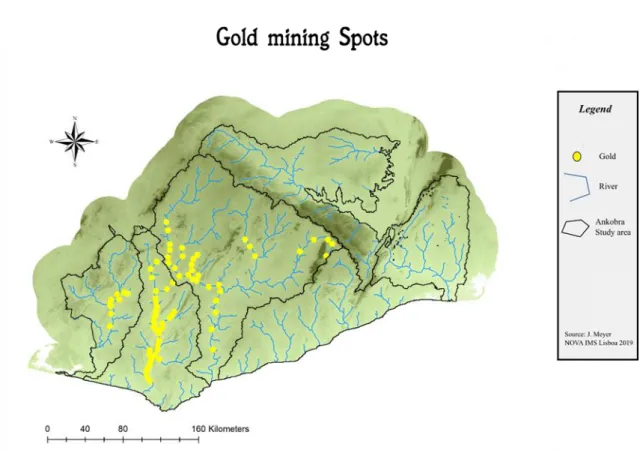
After the identification of the small-scale mining sites, their location was extracted from Google Earth, and imported into a point layer in ArcMap. The locations, the river system and water basins are presented below (Figure 7).
Figure 7 Small scale gold mining spots and river systems
The rivers were selected with the tool Select and a polygon for the
surrounding of the river system was created with “Buffer” and 2km as the buffer-distance.
The “Goldspots” layer was used to create a polygon for the areas where the mining occurs (Buffer with 4km).
Using the tools Intersect and Dissolve, the small-scale gold mining area was determined by overlay the “Goldspots” with their surroundings.
From the LULC 2016 layer, the class for bareland was selected and clipped with the Gold Area to establish the new landcover class “Goldmining.”
25
This was done because it was observed that many lands used for mining activities are classified as bareland within the LULC 2016 dataset. Than the Aggregate tool was used with 9 as the Cell factor and SUM as the Aggregation technique, to get wider areas and exclude single points in favor of a more realistic model of the observed mining area.
For exporting it into the InVEST model, the raster containing the
“Goldmining” landcover class was merged with the background-layer using the tool Mosaic to new raster.
4.2 Methods
4.2.1 Invest
Besides others, (e.g., ESTIMAP, ARIES, Costing nature, LUCI MIMES) InVEST is a commonly applied framework for modeling ES with
standardized methods (Crossman et al., 2013). InVEST is a collection of open access GIS-tools for mapping and evaluating ES, it was developed within the Natural Capital Project. Several standalone models offer a wide range of possibilities for analyzing spatial patterns of multiple ES and their changes during the time based on land cover maps and spatially explicit biophysical variables (InVEST, n.d.).
The goal of the InVest models is to provide information about the impact of changes inside the ecosystems on the related benefits of the people. The prediction of these impacts under alternative land use scenarios and climatic conditions, as well as the evaluation of trade-offs between
ecosystem services and economic sectors, provide valuable information for decision-makers (InVEST, n.d.). Possible questions that Invest can help to answer are for example:
• Where is the source of an ES and where is it consumed? • What is the impact of urbanization or climate change on ecosystem
26
• Or what effect on biodiversity or water quality can be expected from several different forestry management plans?
In concrete, InVEST models are used for supporting applications that estimate the impact on the environment of infrastructure projects, the creation of strategies for sustainable resource supply or the development of sea-level adaption strategies (InVEST, n.d.).
In this study two InVEST models were used, the Nutrients retention and delivery model (NDR) and the habitat quality model (HQ).
The NDR model is evaluating the effects of land use on water quality. By considering the nutrients retaining capacity of the single landcover classes and the surface water flow based on slope, it is calculating a value for the average annual export of the examined substance per raster cell (Niquisse & Cabral, 2017). The HQ model is ranking the landscape based on landcover classes with respect to threats to the biotope and the biodiversity within it (Niquisse & Cabral, 2017).
Based on this previously described framework, it was developed the methodology which is presented in the next section.
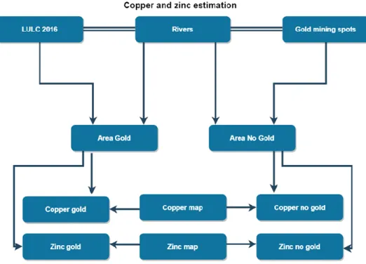
4.2.2 Estimation of Copper and Zink at the Ankobra
Copper and Zinc are heavy metals that are typical of pollution within gold mining areas. Both substances are a natural consistence of the soil and do support metabolic functions inside animals and plants (Sun et al. 2018). To identify pollution caused by gold mining activities within the Ankobra river system, two areas for comparison were defined, one with (“AreaGold”) and one without mining activities (“AreaNoGold”) (Figure 8).
27
Figure 8 Diagram of copper and zinc estimation within the Ankobra river system
The river parts where the small-scale mining sides are located on were extracted from the “rivers” layer with Select. Then around the same size of river-parts within the same river system that are not located in the mining area were extracted. With Buffer the study area is defined as the
surrounding of the river within a distance of 5km. The small scale “Gold-mining spots” point layer was amplified with Buffer by 8km radius and used as the erase feature in the Erase tool, to subtract it from the study area. The resulting layer is defining the area where there is no gold mining. Erase was used one more time to subtract this area from the study area to get the gold mining area (Figure 9).
28 Figure 9 Study area at the Ankobra river
Both layers were then used to clip the “LULC 2016” layer, the “Copper” layer, and the “Zinc” layer using the tool Clip.
Subsequently, Resample was used to transform the two Copper layers (AreaGold and AreaNoGold) and the two Zinc layers to the same cell size that the LULC 2016 layer had. This was done in favor of the processing capability.
The four landcover layers were then split into their single landcover classes by using Extract by Attributes. With Reclassify every one of the resulting layers was rearranged into two classes: 5000 for the value and 0 for
NoData. This enhancement makes the identification of the pixels noticeable later on. Then all the landcover classes were combined by Mosaic to new
layer four times, once with “AreaGold-Copper”, once with
“AreNoGold-Copper,” once with “AreaGold-Zinc” and lastly, once with “AreaNogold-Zinc.” With Extract by attributes tool, all cells with values bigger than 5000 were extracted and the resulting layers tables were saved with Make table view and Table to excel.
29
The next step was to calculate the average values of copper and zinc content for every landcover class both within and without the mining area.
Accordingly, the tables were loaded into Excel where the cells values were multiplied with their occurrence. The sum of all values divided by the number of cells gives the average interstratification of the examined metals within the first 30cm of the soil. The resulting values were ordered into a table and are discussed in the results chapter.
4.2.3 Estimation of Nitrogen (N) and Phosphorus (P)
To estimate the pollution caused by agriculture it is suitable to measure nitrogen and phosphorus. Both are nutrients that can be found nearly everywhere inside the nature. In agricultural landscapes they are deployed as nutrients for fertilization. When the extant of nutrients in water bodies is high, it causes algae to grow faster. This is resulting in decrease in the available oxygen that is needed by the animals inside the water.
The nutrient retention model (NDR) estimates the amount of nitrogen and phosphorus that reach the rivers by modelling the movement of nutrients
through space.
Therefore, it is calculating a raster-based annual water yield by using an elevation model and average precipitation data. This water yield is then combined with coefficients for either nitrogen (N) and phosphorus (P) export for every landcover class to estimate the subsurface flow of nutrients.
As input, it is using average values for every LULC class that represents nutrient loads located on the surface. These values are divided into two parts: One part that is transported with the surface flow which is floating to the rivers, and one part that trickles of
into the sediment.
The flow direction is estimated by a slope map, which is created
automatically out of the DEM by the model. Within the model's control window, the user has to insert a value for the flow accumulation threshold. This value determines the number of
in-30
flowing cells into a cell, from which on the cell itself is considered as part of the flow. The value should be as low as possible, but high enough to identify rivers on the slope map quickly. Below it is presented the slope map for the study area with 150 flow accumulation threshold as used in this study. Another input parameter of the InVEST NDR model is the bulk density of the surface. It determines the percentage of substances that trickle-down into the soil instead of flow away on the surface and is depending on the soils texture and consistence.
The used values represent the average for every landcover-class and were obtained from the literature (Leh et al., 2013).
The study area in Leh et al. (2013), covers the whole of Ghana and the neighboring country Cote Ivoire. It was necessary to transform their values into the corresponding landcover classes. This procedure, the
trans-formation between the base values (Leh et al., 2013) and the used values (“Corresponding LC”) is shown in table 6. While for the value of Forest, just the Tropical Forest was applied, the other values are the average of the corresponding base values for the land cover.
Table 6 Nutrients and phosphorus load per land cover class (adapted from Leh et al, 2013)
As the model's input Nutrients Runoff Proxy, a layer for the average precipitation of the whole year was created. After clipping and projecting,
31
the twelve layers for the twelve months of the year were merged with Mosaic to new raster.
Finally, a “Biophysical table” was created, containing the values for the load of nutrients per raster-cell, the average amount of nutrients that could be stored in the soil for each land cover class, and the maximum travel-distance of nutrients within the single landcover classes. To get obvious values for the nutrients load for each landcover class, two different approaches were used:
The second approach uses average values extracted from the corresponding ISRIC layers with the same procedure than the one done while estimating the bulk density as described before. The resulting values, representing the N and P loads for both the first approach (Database) and the second
approach (Own-data) are shown in Table 7.
Table 7 Values of the NDR “Biotable” (adapted from Leh et al., 2013)
After the estimation of the input values, the InVEST NDR models was equipped. It needs a DEM, a LULC layer, a polygon layer for the water basins and a layer representing the precipitation (“Nutrient Runoff Proxy”) and furthermore, the biophysical table.
Within the model control panel, some adjustments were also needed. It was always used 150 for the “Threshold Flow Accumulation”, 0,5 for the
“Borselli k Parameter”, 75 as the “Subsurface Maximum Retention
Efficiency” (which is the maximum percentage used within the input data)
Name Nitrogen (Datab.) Phosphorus (Datab.) Nitro. (Own-Val.) Phosph.(Own-Val.) Retention-efficency
Forest 3,1 0,1 28,5 5,8 0,75 Shrubs 7,2 0,4 24,7 35,4 0,65 Grassland 5,2 0,4 28,2 40,2 0,62 Cropland 10,2 1,1 31,7 38,7 0,3 Wetland 2,8 0,2 34,4 40,3 0,6 Sparse Veg. 3,4 0,6 29,2 16,2 0,55 Bareland 2 1,3 29,4 36 0,05 Urban 4 2,6 28,5 43,3 0,05 Water 0 0 34,6 36,5 0,02
32
and 20000 as the “Subsurface Critical Length” (which is as well the maximum value used as input).
For the estimation of nitrogen and phosphorus delivery within the small-scale mining areas, the parts of the river system within the area were selected. A comparable area outside the mining area was as well selected (Figure 10). The buffered polygons were used as the mask for extracting values from the results of the NDR model.
Figure 10 NDR inside and outside mining area
4.2.4 Estimation of Mercury (Hg)
Large amounts of Mercury (Hg) are released into the environment as a result of its usage in small-scale gold extraction. For the identification of mercury deliverance from the small-scale gold mining sites, the InVEST
33
NDR model was equipped with its average amount per cell (Figure 10). The model was conducted three times for analyzing the influence of the
precipitation seasons on the mercury release.
Figure 11 Diagram for mercury delivery and retention model
The value for the Hg load was calculated with the amount of gold exported, the gold price (Gold.de, 2019) and the amount of Mercury that is released into nature during the gold extraction. The total amount of produced gold was estimated by comparing the monetary value for the export in 2016, which was 4428 Million US Dollar (World Bank), with the average gold price on the world market for the same year, which was 39775 US Dollar per kg. Therefore, it is:
4428000000
39775 = 111326
This means Ghana exported a total of 111326 kg of gold in 2016. The amount of produced gold within the small-scale mining spots is around 4% of the overall quantity in Ghana (Aragon & Rud, 2012):
111326
100 × 4 = 4453
This complies to 4453 kg gold produced by small-scale mining per year and 12,2 kg every day. The amount of Hg that is going directly into the water, soil, and streams as inorganic Hg and later converted into organic forms is
34
estimated to be around 1,32 kg per 1 kg gold produced (Aragon & Rud, 2012):
1,32 ×12,2 =16,47
The total amount of mercury delivery is about 16,47 kg per day. The next step was to establish a new landcover class for the small-scale gold mining sides. The point layer (“Goldspots”) that was created from the observed mining areas (Chapter 4.1.) was used to identify the rivers on which the pollution is mainly occurring.
The total daily load for Hg (16,47 kg) was now multiplied with the number of days within the desired time-spawns and divided by the number of cells (12287) within the “Goldmining” landcover class:
For the annual runoff the mercury load per cell is 489,26 (g):
16470 × 365
12287 = 489,26
For the rainy-season runoff it is 163,53 (g):
16470 × 122
12287 = 163,53
For the dry-season runoff it is 160,86 (g):
16470 × 120
12287 = 160,85
These calculated values represent the input load per cell for the three-time periods (annual, rainy-season, dry-season) and are inputted into the NDR
35
model. All other datasets (DEM, Precipitation), values (bulk-density,
retention-efficiency) and adjustments within the models control panel were the same than used in chapter 4.2.3.
4.2.5 Habitat quality
In general, habitat quality means the capability of an ecosystem to provide all necessary goods and services in a sufficient amount for all of its living environment (Niquisse & Cabral, 2017). The InVEST habitat quality model, is ranking areas in dependency on their predicted biodiversity. High habitat quality means richness of native species. The model calculates the spatial distance of a habitat to several threats that can be weighted to respect the strength of their impact (Terrado et al., 2015).
For the study area, it is considered as a threat: agricultural land, urban areas, tourism sites, industrial sites, mining sites, small-scale mining sites, streets with high traffic density and streets with medium-high traffic
density.
The locations of gold mining spots and industrial areas were identified by visual research on Google Earth remote sensing imagery. The approach is
explained in Chapter 4.1.
To determine cities and villages, the land cover class “urban” was extracted with ArcMap, transformed into a polygon shapefile and, then classified into either city or village dependent on the size of the dissolved polygon.
Subsequently, the cities were used to eliminate all roads within them and to identify the first order roads that are within a 20km radius around them. All of the remaining roads represent the second order roads layer.
Both the roads layers extents were amplified with Buffer of 500m to determine their threat area and transformed to raster files.
36 Figure 12 Diagram of habitat quality estimation
The roads layer within the cities radius of 20km was merged with the “highways” layer with Mosaic to new raster. “Agriculture” is also the corresponding class in the LULC2016 layer minus the “Cities” layer. To reduce the computing time of the model, the LULC layer was resampled with the tool Aggregate. “Median” was chosen as the aggregation technique to ensure that the most suitable class for the new pixels is selected.
For the InVEST habitat quality model, it was necessary that all input raster
have the same extent.
If the cell contains the specific threat, the value must be 1; if not 0. If there is at least one cell in one of the rasters that has the value “NoData”, the model is running but producing wrong values for all cells. For this reason, it is recommended to ensure that the data frame has the same coordinate system than the threat raster before exporting them to the InVEST model.
37 Figure 13 Threat map
Four factors ascertain the negative effect on the habitat quality that is caused by the threats:
• The relative impact of a threat to any habitat.
• The relative sensitivity of one habitat to any threats. • The distance between habitat and the source of a threat. • A specific value for the impact of a threat to the single habitat
classes.
These values were based on general ecological insights and organized into a table which is one of the input files for the model.
Terrado et al. (2016) performed a study of habitat quality with InVEST in Cataluña, for which they conduct interviews with ten experts of different ecological disciplines, to obtain values as input parameters (Annex F). Their values were slightly modified to apply them to Ghana.
38
Several considerations were done to determine which values should be adjusted. For a brief overview, the impact of the single threats on the habitat quality is described shortly:
• Agriculture is a threat to the materials cycle because of pollution with nutrients and a threat to biodiversity through monoculture. Also, agricultural expansion is more likely to occur close to agriculture.
• High traffic density roads are a threat through exhaust gas
pollution, soil pollution, noise pollution and the danger to animals that cross the street. The probability of destruction of habitat due to urbanization is also increasing nearby highways and main roads close to cities and towns.
• Roads exhibit the same threats than the main roads, but due to the lower traffic density, their extent is much smaller. Based on their locations outside of the main settlement areas, roads are a threat to habitat because they exploit outlands and raise
therefore the probability of deforestation.
• Villages are a threat to habitat because their inhabitants produce wastes that might not get eliminated. Also, they interfere with their surroundings while hunting or timbering.
• The city’s have a better-equipped waste disposing system than villages, but due to their huge population density and existing slum quarters, the extent of waste and waste-water pollution is even greater.
• Tourism is a threat similar to a village but with higher waste production due to the high consumption and short stay time of the single tourists.
• Industry means in this case, locations that cover heavy industry like big fabrics or airports, harbours or big scale mining sites. It is polluting the habitat mainly through air pollution and waste water and is the strongest of all threats to the habitat. On base of these considerations, the sensitivity of the landcover to the single threats was adjusted on base on the values used by Terrado et al.
39
(2016), (Table 8.). The sensitivity of each land cover class to any threat, is represented with a value between 0 and 1.
A second table (Table 9) gives information about the weight of the threats impact in relation to the other. Furthermore, the table contains information about the distance in which the threat is impacting the habitat and if the decay of the impacts strength is linear or exponential.
Both tables are in CSV format, using “;” as a delimiter between the columns and “.” between numbers (the U.S.-American delimiter style).
Table 8 Sensitivity of landcover to threats
Table 9 Threat table
Land Cover Agriculture Highways Roads Villages Cities Tourism Industry Gold
Forest 0,7 0,8 0,8 0,75 0,75 0,55 0,7 0,7 Shrubsland 0,7 0,8 0,8 0,75 0,75 0,65 0,7 0,7 Grassland 0,7 0,7 0,7 0,75 0,75 0,75 0,7 0,7 Cropland 0,1 0,6 0,6 0,7 0,7 0,7 0,9 0,8 Wetland 0,7 0,3 0,3 0,5 0,5 0,4 0,9 0,8 Mosses 0,7 0,7 0,7 0,75 0,75 0,75 0,7 0,6 Bareland 0,7 0,7 0,7 0,75 0,75 0,75 0,7 0,6 Urban 0,2 0,1 0,1 0,1 0,1 0,3 0,5 0,5 Water 0,9 0,8 0,8 1 1 0,5 1 1
THREAT Max. Distance Weight Decay
Agriculture 4 0,68 exponential Streets 2,9 0,71 exponential Roads 2,9 0,36 exponential Villages 3,6 0,5 linear Cities 7,1 1 linear Tourism 3,6 0,5 exponential Industry 8 1 linear
40
5. Results
5.1. Copper and Zinc
As explained in chapter 4.2.2., it was calculated the average copper and zinc content of the most near-ground soil layer for both the small-scale gold mining sites and a neighboring, comparable area. Both areas were split into landcover categories to get an insight into the impact of heavy metal
pollution caused by gold mining on different land cover. The results are presented in table 10.
Table 10 Zinc and Copper content in mg/100kg
The total extent of the Area Gold is 2449,95 km², and the size of Area No Gold is slightly bigger with 2619,95 km². Both Areas are covered mostly by forest and cropland.
Interesting is that the values of forest are above average, while its values must be equated the most because of its vast size and forest is located mostly at the margins of the study area.
Bareland is the landcover class where most mining areas are classified. It is bigger in the area without gold mining, but its values for zinc is much less than inside the mining area.
41
When subtracting the values of the “No Gold” area from the “Gold” area (Table 11), it gets visible that wetland and the small content of urban are more polluted outside the mining area. All other land cover classes and as well the total study area contain higher amounts of zinc and copper within the mining area.
Table 11 Differences of heavy metals in mg/100kg
LC Difference (Zinc) Difference (Copper)
Forest 13,2 3,25 Shrubs 3,21 2,98 Grassland 4,44 -2,45 Cropland 9,79 -1,49 Wetland -9,59 -12,12 Sparse veg. 0 0 Bareland 31,66 -0,57 Urban -31,78 -25,14 Water 0,15 -2,6 Total 5,43 1,88 5,4345334 1,8826494
42 Figure 14 Soil zinc content
43
In the maps for the copper and zinc content of the highest soil layer above the surface (Figure 14 and Figure 15), it is visible that the content of both heavy metals is higher in other areas. The cities Accra and Kumasi show higher content. This means that it is possible to identify pollution of heavy metals with soil layers, but not all differences of heavy metal content are a result of pollution
On base of this approach it can be declared, that coherence between heavy metal pollution and gold mining activities is being established.
5.2. Nitrogen and Phosphorus
By using 1 as the input data for all the landcover classes, it was possible to test the behavior of the NDR model when the difference between the single landcover classes would not be respected. It was a big range within the values visible, as well as dependency to the height and even more to the river systems.
The following map illustrates the results of the NDR model for Nitrogen and Phosphorus delivery. The values indicate the amount of the examined substances that is reaching the stream and therefore will flow into the ocean.
44 Figure 16 NDR Nitrogen (Annual)
On the map (Figure 16), it is visible, that:
• There is a wide range of values from close to zero up to 17 grams per 100 kilograms of annual nitrogen retention.
• The peak of values is in the agricultural region, that is located southern of the Lake Volta in the south-east.
45 Figure 17 NDR Phosphorus (Annual)
Above (Figure 17) it is presented a map that shows the result of the NDR model for the annual phosphorus retention. There it is visible, that: • There is again a wide range of values from close to zero up to 4,2
grams per 100 kilograms of annual phosphorus retention.
• The peak of values is again in the agricultural region, that is located southern of the Lake Volta in the south-east. And as well inside the metropolitan areas Kumasi and Accra.
• In general, the spatial pattern is highly unallocated. Within huge areas, the retention is close to nothing.
46
5.3 Mercury
The results of the approach estimating the mercury retention and delivery (which is explained in chapter 3.4.) is a spatial dataset, as the output of the InVEST NDR model.
Figure 18 Mercury delivery (Annual)
The model was used with different precipitation layer, one for the rain season (November to February) and one for the dry season (April to July). When comparing the model´s results for both seasons (Annex E) with the results for the whole year, there are slight differences in the distribution of the amount of delivered mercury visible. Within the whole year (Figure 18) the spatial pattern shows that the highest amount is occurring on the Ankobra and the Upper Pra with its peak in the centre of the Ankobra.
47
The spatial pattern for the two seasons shows that the amount is higher during the rain season, but this in different extent: While the seasonal difference is high on the Upper Pra, it is low on the Ankobra. The reason therefor must be differences in the water yield between the two streams. While the amount of water in the Ankobra is diverse only in its upper part close to its source, the Pra contains obvious more water during the rain season.
5.4 Habitat Quality
The result of the InVEST Habitat Quality model is presented in Figure 18. For the estimation of habitat quality within and without the small-scale mining area, it was necessary to cut the habitat quality models output to size. The green lines in Figure 19 represent the borders of both areas: Within and without the mining area.
48
The habitat quality is displayed with a range between red and blue, where red means low quality (Figure 19). While interpreting the map, it is visible that the significant metropolitan areas of Kumasi and even more of Accra are the worst habitats within the study area. The main agricultural region, located south-western of the lake Volta, also shows low habitat quality.
Figure 20 Habitat quality within and without the mining area
Based on the resulting layer (Figure 19), the study area was ranked into ten classes that represent their habitat quality (Figure 20). The quality within the mining area is less high, but the worse habitats are outside of the buffer.
When ranking the whole study area, a wider overview is showing up (Figure 21). The highest habitat quality is located within the north-east and the western border of the study area. The reasons, therefore, are a high amount of forest, a low population density, and the absence of industry.
49 Figure 21 Classified Habitat Quality
The nature reserves are protected areas that show a habitat quality higher
than the average within the study area.
In general, the coast shows less habitat quality than the mainland, but the mining areas are visible as a strip from the coast to Kumasi with less high
quality.
While Accra shows the lowest habitat quality within the study area, Kumasi shows a distinctly higher level. The main reason, therefore, is probably that there are much more streets around the city than in Kumasi. This fact is visible on the threat map (Figure 13) and can be explained with the low density of buildings within this area. That is why the landcover is interpreted within the LULC layer as “Grassland” and as “Cropland” instead
of as “Urban”.
Another reason is the shape of the cities suburbs, which is more or less round in Accra and more or less radial in Kumasi. While buffering and
50
generalizing the road network of this suburbs (which was done while
transforming the lines from the vector into raster cells), the resulting threat layer is bigger around Accra.
Based on this background, it is possible to declare that gold mining is a relatively high threat to the habitat, because:
• Most industrial activities outside the metropolitan areas are gold mining.
• The small-scale gold mining is permanently destroying river banks and polluting water that streams down the landscape
• Settlements and streets are over proportional located near gold mining areas.
Even when keeping in mind that the output is depending on the input and the adjustments done within the threat and sensitivity table, the habitat quality map can add some other insights to ES studies and the relation between ecosystems and anthropogenic land use. For example, within the study area, the spatial view shows that industry and tourism are less critical threats to many habitats. This is because of the locations of the threats within the densely populated coast and in Kumasi.
5.5 Comparison of model results inside and outside gold mine areas
For the identification of the impact of gold mining on the ecosystem, it is useful to compare the mining area with its surroundings like it was done in this work. Table 12 shows an overview on the results of the different