Advanced probabilistic load flow

Tomasz Ciereszko

Cálculo do Fluxo de Potência Usando

Métodos Probabilísticos

Advanced Probabilistic Load Flow

Probabilistyczne podejście do obliczania

przepływów mocy w sieci energetycznej

Tomasz Ciereszko

Cálculo do Fluxo de Potência Usando

Métodos Probabilísticos

Advanced Probabilistic Load Flow

Probabilistyczne podejście do obliczania

przepływów mocy w sieci energetycznej

Dissertação apresentada à Universidade de Aveiro para cumprimento dos requisitos necessários à obtenção do grau de Mestre em Engenharia Electrónica e Telecomunicações, realizada sob a orientação científica do Prof. George Anders, da Lodz University of Technology, Polónia e co-orientação científica do Doutor Rui Manuel Escadas Ramos Martins, Professor Auxiliar do Departamento de Engenharia Electrónica e Telecomunicações da Universidade de Aveiro e colaboração do Doutor Carlos Alberto Bastos, Professor Auxiliar do Departamento de Engenharia Electrónica e Telecomunicações da Universidade de Aveiro.

agradecimentos I would like to thank my supervisors, parents and friends for all the support and guidance I received from them. Without it, my stay in Portugal would not be so rich.

o júri

Presidente Joaquim João Estrela Ribeiro Silvestre Madeira

Professor Auxiliar do Departamento de Electrónica, Telecomunicações e Informática da Universidade de Aveirorofessor XXXXX

Vogais Marcin Janicki

Professor of Department of Electrical, Electronic, Computer and Control Engineering of Lodz University of Technology

Carlos Alberto Bastos

Professor Auxiliar do Departamento de Electrónica,

Telecomunicações e Informática da Universidade de Aveiro

Rui Manuel Escadas Ramos Martins

Professor Auxiliar do Departamento de Electrónica,

keywords Probabilistic Load Flow, PLF, Load Flow, LF, Sequence Operation Theory, SOT, Energetic Power System, Addition-Type-Convolution, Subtraction-Type-Convolution, Sequence-Multiplication-Operation

abstract This thesis sets forth a computational framework of probabilistic load flow analysis taking into consideration of high penetration of variable energy resources, such as the wind generation. The framework enables a faster and more precise estimation of the impact of variable energy resources in load flow analysis.

This thesis consists of six chapters: introduction, probabilistic load flow algorithms, computer program for PLF calculations, conclusion and future work, appendices and reference.

The second part contains the mathematical development of the framework based on Sequence Operation Theory newly established. The formulation is novel in that it provides an improved computational alternative to the existing simulation based frameworks.

The third part contains information about program written in Fortran 90/95 environment like format of reading data etc. Include the studies based on the standard IEEE 9-bus system. Data obtained as a result of program’s work in debugging process are compared with manual calculations for the same network to check if the program is working in proper way. Moreover comprise the results obtained in the program for largest tested network 96-RTS (24 buses).

Appendices include content of two input files (random generation, system configuration for 96-RTS) and intermediate result calculated for the 24-bus system.

resumo Esta dissertação descreve parte do desenvolvimento de uma aplicação de software para calcular o fluxo de potência em sistemas de redes elétricas usando métodos probabilísticos, considerando o caso da existência de geradores com produção fortemente variável, como acontece nas quintas eólicas.

A dissertação está dividida em seis capítulos: introdução, algoritmos de fluxo de potência probabilísticos, desenvolvimento do código, conclusão, apêndices e referências.

A segunda parte é constituída pelo desenvolvimento matemático do método utilizado, que foi recentemente criado apresentando uma alternativa mais eficiente às tradicionais.

A Terceira parte contem informação sobre a o programa criado para implementar o algoritmo e seu teste, nomeadamente o desempenho na análise do standard IEEE 96-RTS (24 - bus system).

Os apêndices incluem o conteúdo dos ficheiros de entrada e resultados intermédios para debug da solução apresentada.

streszczenie Praca przedstawia probabilistyczną metodę do obliczania przepływów mocy w sieci energetycznej z szczególnym uwzględnieniem zmiennych źródeł energii takich jak generacja wiatrowa. Prezentowane podejście umożliwia szybsze i bardziej precyzyjne oszacowanie zmiennych zasobów energetycznych w analizie rozpływów mocy.

Dokument został podzielony na sześć następujących części: wstęp, algorytm probabilistic load flow, program komputerowy, podsumowanie i możliwośći rowoju projektu, dodatki, bibliografia. Druga część pracy zawiera założenia metody Sequence Operation Theory (SOT). Prezentowany algorytm jest nowy i stanowi alternatywę dla dotychczasowo stosowanych metod.

Część trzecia opisuje program komputerowy z zaimplementowaną metodą SOT stworzony na potrzeby tej pracy. Kod programu został napisany w środowisku Fortran 90/95. Rozdział zawiera badania oparte na systemie sieci energetycznej 9 magistral w celu sprawdzenia poprawności działania kodu. Ponadto w tej części zostały zaprezentowane wyniki działania aplikacji dla systemu testowego 96-RTS (24 magistral).

W dodatkach zaprezentowano zawartość dwóch plików wejściowych: konfigurację systemu testowego 96-RTS i wartości generacji dla zmiennego źródła oraz pośrednie wyniki obliczeniowe dla tego systemu.

LIST OF FIGURES

Fig. 1.1 Example of electric power system ... 1

Fig. 2.1 Discretized sequence of random variable ... 10

Fig. 2.2 The 3-bus System of the numerical example ... 19

Fig. 2.3 Probability sequence of generation at Bus 2 ... 23

Fig. 2.4 Contribution of the random generation at bus 2 to the flows in lines 1, 2, 3 ... 25

Fig. 2.5 The total line flows on lines calculated using ATC ... 26

Fig. 2.6 The total line flows on lines calculated using STC ... 26

Fig. 3.1 The 9-bus System of the Example ... 34

Fig. 3.2 Probability sequence of generation at Bus 2 ... 37

Fig. 3.3 24-bus IEEE Test System ... 43

Fig. 3.4 The contribution of random generation at buses 2 and 15 on the flows in transmission line 6 ... 44

Fig. 3.5 The contribution of total line flows and generation at bus 2 on lines 1-7 ... 45

Table 2.1 Example of Probability Sequence ... 11

Table 2.2 Examples of Sequence Operations ... 14

Table 2.3 Impedance of the Transmission System ... 19

Table 2.4 Generation and Load Information ... 19

Table 2.5 Sequences of Generation Shift Factor of Bus 2 for Line 1, 4 and 6 ... 24

Table 3.1 Impedance of the Transmission System ... 34

Table 3.2 Generation and Load Information ... 35

CONTENT

1. INTRODUCTION... 1

2. PROBABILISTIC LOAD FLOW ALGORITHMS ... 3

2.1. Load Flow ...3

2.2. Traditional probabilistic Load Flow problem ...5

2.2.1. Mathematical model ...5 2.2.2. Example of solution ...7 2.3. Sequence Operation... 10 2.3.1. Definition of sequence... 10 2.3.2. Addition-Type-Convolution (ATC) ... 12 2.3.3. Subtraction-Type-Convolution (STC)... 12 2.3.4. Sequence-Multiplication-Operation (SMO) ... 13 2.4. Power equations ... 15

2.5. Random Inputs and Probabilistic Load Flow Calculation ... 16

2.6. SOT Based Computational Framework ... 17

2.6.1. Process I. Data preparation ... 17

2.6.2. Process II. Discretization ... 17

2.6.3. Process III. Sequence operation ... 18

2.6.4. Process IV. Analysis ... 18

2.6.5. Numerical Example with a 3-bus Test System ... 18

3. COMPUTER PROGRAM FOR PLF CALCULATIONS ... 27

3.1. Implementation ... 27

3.1.1. Data preparation ... 28

3.1.1.1. Inputs ... 29

3.1.2. Discretization ... 32

3.2. Tests on 9-bus system... 33

3.2.1. Data and manual calculations ... 33

3.2.2. Debug process ... 38

3.2.3. Output ... 42

3.3. 24-bus IEEE Test System ... 43

4. CONCLUSION AND FUTURE WORK ... 47

4.1.1. Conclusion... 47

4.1.2. Future work ... 47

5. APPENDICES ... 49

5.1. Appendix A ... 49

5.1.1. Random generation file for the 24-bus system ... 49

5.1.2. System configuration file for 24-bus system ... 49

5.2. Appendix B ... 54

5.2.1. Intermediate results ... 54

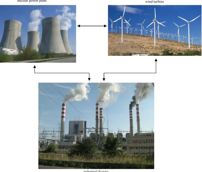
nuclear power plant _{wind turbins}

industrial factory

1. INTRODUCTION

A electric power system is a network of electrical components used to supply and transmit electric power. Computation of power flows in the electric power system is one of the major tasks facing power system planners and operators. At the beginning of the electric utility industry, the power flows in transmission lines were computed by engineers with the help of a slide rule, pencil and a piece of paper. They could spend days to analyze power flows, generation conditions and setting up system configuration. Situation has changed with the advent of digital computers. New technology allows analysis of more complex systems and also a study of the effects of power system faults. The illustration of power system with two different generations (power station and wind turbins) and one kind of load (factory) is illustrated below:

Furthermore, nowadays we can study future system conditions, which give confidence in making judgments concerning investment and operating decisions. However, future operating conditions can never be stated precisely, and many phenomena governing the design and operating criteria of the power systems cannot be predicted with certainty. Electric power systems are designed to survive bad weather condition, short-circuit current and possible unit outages. High-voltage systems consist of many components and the state of each of it can be uncertain. In the past, engineers used deterministic methods to analyze and design power systems. Modern systems are much bigger, more complicated and very often include renewable sources, output of which is depended on the wind and solar conditions. Thus, one can argue that nowadays deterministic methods are insufficient. In designing new power systems, engineers have to work with the unknown future load and generation conditions as well as with the unknown equipment conditions. This justifies a replacement of traditional analysis methods by more rigorous ones based on formal mathematical techniques and reliability theory. The most popular approaches for modeling uncertainty are probabilistic methods.

Probabilistic Load Flow (PLF) has been often used to study the impact of uncertainties [7] such as those from load and forced outages. For example, [12] has reported an application of PLF in calculation of available transfer capability of transmission lines; [5] has used PLF for transmission system expansion analysis. Application of PLF in short-term planning and operation has also been explored, as those in [9],[10]. In addition, PLF can be used for distribution system analysis as well, as suggested by [11]. Recently, there is a growing interest in applying PLF to understand the impact of resource-side uncertainties from renewable generations on the power system operation [13].

2. PROBABILISTIC LOAD FLOW ALGORITHMS

The load flow study involves the steady-state simulation of a power system. The deterministic load flow is used to analyze and appraise the power system. Inputs contain data of the real and reactive loads at load buses, real power generation and voltage magnitude at generation buses. As a result of the calculations, we obtain voltage magnitudes and angles at the load buses, angles and reactive power demand at the generating buses and active and reactive power flows in the transmission lines. It is important to underline that this method ignores several uncertainties, including the change of network configuration or outage rate of generators. Moreover, more often, renewable energy is exploited in the hi-tech power systems. Unfortunately, wind turbines and photovoltaic systems provide additional uncertainties into the system due to their uncontrollable prime sources. Thus, deterministic load flow may results in an unrealistic state estimation. In order to take into consideration many uncertainties, a probabilistic approach can be used.

The first approach to the Probabilistic Load Flow (PLF) analysis was proposed by Borkowska in 1974 in [4]. The idea is to incorporate uncertainties in available generation and load in the analysis. The goal is to obtain the distributions of the state variables and line flows through repeated calculations of the load flows to support decisions under uncertainty. The PLF can be solved numerically or analytically.

A numerical approach is a process in which we select a set of values of system parameters and as a result obtain a solution of the system model for a selected set. Repeating this process for different sets of system parameters we obtain different sample solutions. The main aim of this process is to obtain sample solutions by the selection of representative sets of system parameters. The most popular numerical approach is the Monte Carlo (MC) method. The two main features of the MC simulation are random number generation and random sampling. Software such as MATLAB provides algorithms for pseudorandom number generation. Probabilistic Load Flow calculations using MC approach involves performing deterministic load flow studies many times for different combinations of the nodal power values. Using the MC approach, we can obtain accurate results with an application of the non-linear LF

equations. Unfortunately, this method has some limitations. The random sampling demands a large number of iterations to maintain the desired accuracy, which is very time consuming.

The basic idea of the analytical approach proposed by Borkowska is to use a convolution method with probabilistic density function of stochastic variables of the power inputs. Unfortunately, there are some difficulties of using this approach, because this method has the following assumptions that are needed to solve practical cases:

 Linearization of the Load Flow equations.

 Total independence of linear-correlated power variables.

 Normal and discrete distributions are usually assumed for load and generation.  Network parameters and configuration are constant.

Very often, Load Flow equations are non-linear and power inputs at different buses are usually not completely independent.

Because of the complexity of the convolution method, another approach involving so called Sequence Operation mathematical tools is proposed and discussed in section 2.3. In that work

2.2. TRADITIONAL PROBABILISTIC LOAD FLOW PROBLEM

This section describes a method for evaluation power flow which takes into consideration uncertainty proposed by Barbara Borkowska in [4]. Calculation are used for networks with constant configuration and line parameters. The aim of the method is to compute the probability distributions of the line flows given random loads and generation at some buses.

2.2.1. MATHEMATICAL MODEL

The mathematical model of this approach is presented below:

Pn – random vector of power inputs and outputs.

It is assumed that distribution function Fni of mutually independent random variables Pni is known.

The first step is to obtain a random vector of net power inputs. We define a transformation matrix T of order NxR as follows.

T – transformation matrix of order NxR, the elements of this matrix are equal to zero or

to one according to definition below:

1 for P

∈ P

0 for P

∉ P

Because Pni belongsto one node only:

= 1 = 1,2, … ,

PN – random vector of net nodal loads is therefore given by:

P

= T P

Since branch flows are linearly related to the net nodal loads and active and reactive power flows are independent of each other.

P

= A P

where:

PB – vector of branch real power flows

PW – vector of nodal real powers

A – transformation matrix of order BxN (B - number of branches, N – number of nodes)

A = [A

|0]

Ao – transformation matrix of order Bx(N-1)

A

= Z

C (C

Z

C)

ZB – matrix of moduli of branch impedances

C – connection matrix

The sum of nodal real powers must be equal to zero since the losses are neglected.

∈

P

= 0

P

= P

– P

S =

∈

P

= ∈

P

or outputs)

S – the balance of power in the network

Let consider two possibilities S can denote the deficiency or surplus of power. If S denotes deficiency the vector PL is the vector of the deficiency distributed among the particular nodes and if S denotes surplus of power the vector PL is a vector of the reserve capacity distributed among the nodes. That is why it may be written as:

P

= ɸ(S)

Taking into account equation PB = A Pw we get

P

= A (P

- ɸ(S))

In the above equation all data on the right side are known. We can calculate the vector of unknown branch flows - PB.

2.2.2. EXAMPLE OF SOLUTION

FBj for j = 1, 2,…B) – distribution function of the branch flows PBj

N – number of nodes

B – number of branches

R – number of distribution function of active power inputs or outputs

i – distribution number

j – branch number

k – node number

Taking into account the calculation from Section 2.2.1, it may be written:

P

= G

– Ψ(S

)

Where

G

= ∑

∑

T

P

Ψ(S

) ∑

ɸ

(S)

The random variables GR and SR are dependent

G

= G

+ W

P

where

W

= ∑

T

G

= ∑

P

S

= ∑

G

= W

P

S

= P

Thus the distribution function FGS1 of the variables (G1,S1) is given by:

F

(W

β, β) = F

β

Because (G1, S1) and Pn2 are mutually independent then

F

(g,s) = ∫

(g - W

β, s – β) dF

(β)

Since

G

= G

+ W

P

S

= S

+ P

For i = 2, 3, …, R

F

(g,s) = ∫

(g – W

β, s – β) dF

(β)

If the distribution function FGSR is known then the density function fGS of the random variables (GR, SR) is:

F

(g,s) =

( , )

F

(g) = ∫

∫

(g - Ψ(s), s) ds dg

The evaluation of FGSR is simpler and less time consuming if the function ɸ(S) is linear.

ɸ(S) = L

S

Then it can be written

P

= H P

H = A(E - L

∈

) T

P

= ∑

P

P

= H

P

P

(H

β) = F

(β)

P

= P

+ H

P

F

(γ) = ∫

(γ - H

β) dF

(β)

As we can see method for PLF proposed by Borkowska is based on probability convolution. However, the initial analytical formulation is too complicated to be directly used in practice for large networks [Section 2.1]. Therefore, a large number of research works have been devoted to the development of simplified computational frameworks, so that PLF can be effectively used to solve complicated practical

problems. One of the challenges of simplification is to find an appropriate tradeoff between accuracy and the efficiency of computations. One such approach using a tool of sequence operation is discussed in this thesis.

2.3. SEQUENCE OPERATION

Sequence operation is a new computational idea: the distributions of input random variables can be represented by sequences, and the major arithmetic operations can be completed through a number of standard sequence operations using the proposed operators, which will be introduced in next subsection. This approach was fist discussed in [2],[3].

2.3.1. DEFINITION OF SEQUENCE

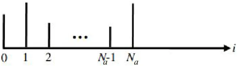
Sequence a(i), i = 0, 1, 2, 3, …, Na is defined as a series of numerical values that begins from 0 and ends with Na (the biggest number, which is called the length of a sequence a(i).)

The example of discretized sequence of random variable is shown in the picture below,

FIG. 2.1 DISCRETIZED SEQUENCE OF RANDOM VARIABLE

Where the height of vertical line contains the information of probability of random variable.

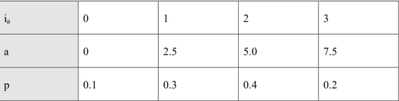
Probability sequence can then be created based on the probability distribution, or the likelihood estimated from the historical observations, of the underlying random variable. More specifically, a probability sequence is a set of indexed pairs of magnitude and its probability density of the underlying random variable, as shown in Table 2.1. The difference between two consecutive points is referred as “sequence interval”.

a a

TABLE 2.1 EXAMPLE OF PROBABILITY SEQUENCE

ia 0 1 2 3

a 0 2.5 5.0 7.5

p 0.1 0.3 0.4 0.2

In Table 2.1 ia is sequence number (ia = 0,1,2,3) for a probability sequence a(i); a is a random variable and p is the corresponding probability. For example in column 5, the probability for the magnitude being 7.5 is 0.2. In this probability sequence, the sequence interval is 2.5, which is the difference between two consecutive points of a(ia+1) and a(ia).

As will be shown in the following sections, sequence operation provides a number of flexible computation methods for operation on random variables. Unlike discrete convolution which only deals with addition/summation of random variables, with the sequence operators described below, addition, subtraction, multiplication, division and other logic operations can all be realized systematically.

The line flows can be computed using the Sequence Operation algorithms. These algorithms use Addition Type Convolution (ATC), Subtraction Type Convolution (STC) and Sequence Multiplication Operation (SMO). SMO can be used to compute line flow contribution from each bus. If we want to calculate aggregation of net injected power we can use ATC or STC The algorithms and their applications are described next.

2.3.2. ADDITION-TYPE-CONVOLUTION (ATC)

ATC operator is used for addition of discrete random variables. It was originally discussed in [2]. Let a(i) and b(i) represent two discrete sequences with length Na and Nb, the addition of the two sequences, x(i), can be represented by Addition Type Convolution defined as follows:

( ) = ( ) ⊕ ( ) where ⊕ is the symbol representing ATC operator.

The ATC operator (⊕) performs the following discrete operation,

( ) = ( ) ( ), = 0,1,2, … ,

Where Nx= Na + Nb.

In the ATC operation, the ith element in x(i) is the summation of the multiplication results for all elements in a(i)and b(i) which satisfy ia + ib = i.

2.3.3. SUBTRACTION-TYPE-CONVOLUTION (STC)

STC operator is used for subtraction of discrete random variables. It was originally discussed in [2]. For two discrete sequence a(i) and b(i), the result of subtraction, y(i), can be obtained by the Subtraction Type Convolution as follows:

( ) = ( ) ⊖ ( ) Where ⊖ is the symbol representing STC operator.

Without loss of generality, assuming Na ≥ Nb, the STC operator (⊖ ) completes the follow discrete operation,

( ) = ⎩ ⎪ ⎨ ⎪ ⎧ ( ) ( ), 1 ≤ ≤ ( ) ( ), = 0

Where Ny = Na.

In the STC operation, the first element y(0) of the sequence y is equal to the summation of multiplication of all elements in a(i) and b(i) which satisfy ia ≤ ib; while other elements in y can be obtained by summarizing the multiplications of all elements in a(i) and b(i) which satisfy ia - ib= i.

2.3.4. SEQUENCE-MULTIPLICATION-OPERATION (SMO)

SMO operator is for multiplication of discrete random variables, including deterministic ones or constants. Consider the two discrete sequences a(i) and b(i), with length Na and Nb, sequence interval Δ and Δ , respectively, the multiplication result, s(i), can be obtained through Sequence Multiplication Operation defined as follows:

( ) = ( ) ⊚ ( )

where (⊚ ) is the symbol of the SMO operator. The SMO operator ( ⊚ ) completes the follow discrete operation,

( ) = _⋅ ( ) ( ), = ⋅

0, ℎ

The dimension of the new sequence Ns= Na· Nb, and the sequence interval Δ ̅ = Δ ⋅ Δ .

In the SMO operation, the ith element in s(i) is the summation of the multiplications of all elements in a(i) and b(i) which satisfy the condition that ia · ib = i, otherwise s(i) = 0.

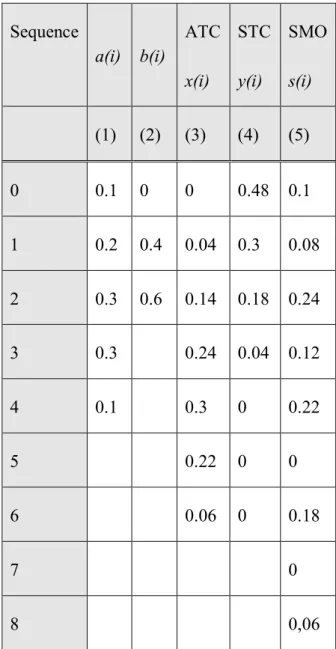
Table 2.2 provides several examples of applying ATC, STC and SMO operations on two arbitrarily given discrete sequences of a(i) and b(i), with lengths of 4 and 2, respectively. The numerical results, i.e., resultant probabilistic sequences, are calculated and presented in column 3, 4 and 5.

TABLE 2.2 EXAMPLES OF SEQUENCE OPERATIONS Sequence a(i) b(i) ATC x(i) STC y(i) SMO s(i) (1) (2) (3) (4) (5) 0 0.1 0 0 0.48 0.1 1 0.2 0.4 0.04 0.3 0.08 2 0.3 0.6 0.14 0.18 0.24 3 0.3 0.24 0.04 0.12 4 0.1 0.3 0 0.22 5 0.22 0 0 6 0.06 0 0.18 7 0 8 0,06

Examples of calculations are presented below:

The number in row 3 and column 5 of Table 2.2 is the magnitude of the product of sequence a(i) and b(i), which is equal to 0.24 and the sequence number is 2. This number is equal to a(1)×b(2) + a(2)×b(1) = 0.2×0.6 + 0.3×0.4, according to SMO calculation introduced before.

The number in row 2 and column 3, which is equal to 0.04 and the sequence number is 1. This number is equal to a(0)×b(1) + a(1)×b(0) = 0.4×0.1 + 0.2×0, according to ATC calculation introduced before.

The number in row 4 and column 4, which is equal to 0.04 and the sequence number is 3. This number is equal to a(4)×b(1) + a(3)×b(0) = 0.1×0.4 + 0.3×0, according to STC calculation introduced before.

2.4. POWER EQUATIONS

Power equations in a DC load flow model for a system with N buses and NT lines can be written as,

, = , ; = 1, … , ; = 1, … ,

Where Pl,T is the active power flow in transmission line l, Pk is the net power injection at bus k, and Gl,k is the generation shift distribution factor (GSDF) of bus k on line l.

DC power equations in a matrix form can be written as,

ℙ = ℙ

in which PT is a NT –dimensional vector of the line flows, PSP is a N-dimensional vector for the net injected powers. G is a NT×N dimension matrix of GSDF, which can be calculated once the line impedances of the power system are known. Calculation of Generation Shift Factor matrix is discussed in Section 2.6.5.

For each transmission line l, the line flow, Pl,T, can be found in a procedure consisting of three steps:

Step 1) Aggregation of total loads and total generations at each bus to obtain net inject power Pk;

Step 2) Calculation of line flow contribution of net injected power at each bus, i.e., Gl,k Pk, for k=1,2,…,N;

2.5. RANDOM INPUTS AND PROBABILISTIC LOAD FLOW CALCULATION

In PLF analysis, net injected power, Pk, at each bus represents power generation, load or the difference between the two.

Variable generation such as that from the renewables can be represented by a random variable. In Step 1 of the DC load flow analysis, if multiple variable generations are connected to the same bus, the total generation can be computed with the ATC operation.

Similarly, aggregation of multiple variable loads at a load bus can be obtained with the ATC as well. It should be noted that the input variables are assumed to be independent in this framework.

For a bus having both the generation and load connected, the net inject power is the difference between the total generation and the total load. This difference can be computed using the STC operator. ATC and STC are also used to compute the total line flow later in Step 3. The line flow contribution of the net injected power at each bus is a function of all generations and loads connected to this bus, which could be a random variable if any generation or load is random.

SMO or Matrix SMO is used for the calculation of the line flow contributions in Step 2. It is worthwhile to point out that, in addition to the application in estimation of load flow impacts from uncertain load and variable generations, sequence operation can also be used to study the impact of forced outages of generation or transmission lines. For example, a two-state outage model that is often used to represent the availability of generation or the status of transmission lines can be discretized into a two-state discrete sequence [FOR, 1-FOR], where FOR stands for a Forced Outage Rate. Thus, the impact of outages on line flow, ΔPl,T, can also be calculated through the sequence operations.

2.6. SOT BASED COMPUTATIONAL FRAMEWORK

The PLF computational framework described above includes four processes: Data preparation, Discretization, Sequence Operation, and Analysis.

2.6.1. PROCESS I. DATA PREPARATION

Data preparation refers to the work of developing a load flow model, obtaining the probability distributions of the random load or generation, and obtaining model parameters including line impedance or generation shift factors, etc. Data preparation is an essential part in almost every PLF framework.

2.6.2. PROCESS II. DISCRETIZATION

Discretization is to create sequences of input variables. In addition, several parameters describing a sequence; such as, sequence interval, starting point and ending point etc., are also defined in this process. These parameters may affect the sparsity and the length of sequence, as well as the smoothness of the resultant distributions. Fortunately, similar to determination of the step length in numerical calculation, these parameters can be easily found or adjusted. The general criterion for determination of an appropriate step length is relatively simple in sequence operation comparing to those for many other numerical algorithms. For a probability sequence of input random variables whose distribution function can be expressed by analytical functions, there commended initial step length of a sequence can be determined in such a way that the step length is around 1/10th to 1/20th of the standard deviation of the underlying input random variable. For those probability sequences that are obtained based on numerical estimation, e.g. histograms, without known parametric form, the initial step length should be chosen close to the smallest step length of the corresponding histogram because it determines the step length or the accuracy of the results. In the sequence operation based PLF framework, all random inputs and constants need to be discretized. For a random input, discretization creates a probability sequence with the method of a deterministic variable, such as generation shift factor, creates a deterministic sequence.

2.6.3. PROCESS III. SEQUENCE OPERATION

Sequence operation is used to compute line flow applying ATC, STC and SMO operators. SMO can be used to compute the line flow contribution from each bus, while ATC and STC can be used for aggregation of the net injected power or calculation of the total line flow once all line flow contributions are known.

The result of sequence operation is a sequence vector that consists of the probability sequences of the line flows. These sequences can be converted to probability distributions similar to those obtained with the Monte Carlo simulation.

However, with sequence operation, the distributions are obtained in a structured, analytical-like approach; and computation time is dramatically reduced without compromising the accuracy.

2.6.4. PROCESS IV. ANALYSIS

This part is common for all PLF computational frameworks, which is to calculate the distributions of line flows, evaluate steady-state reliability indices of interest, conduct related contingency analysis. Since each element in a sequence vector is a sequence, it can be converted to a set of probability distributions. Once the corresponding distributions are known, the conventional methods can be used to evaluate various reliability indices under uncertainty. The example below demonstrates how the sequence operation can be applied to the PLF analysis.

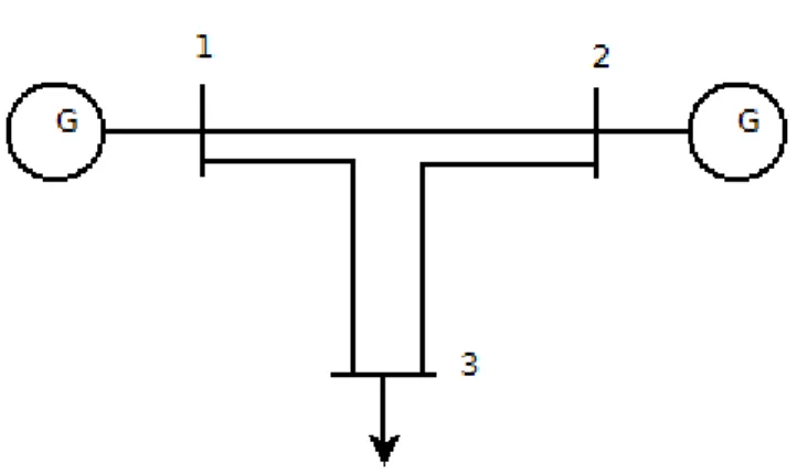
2.6.5. NUMERICAL EXAMPLE WITH A 3-BUS TEST SYSTEM

The studies presented below are based on a 3-bus system as shown in Fig. 2.2. Under consideration are two generators located at bus 1 and bus 2, and one load located at bus 3. Bus 1 is assigned to be the slack. Slack Bus is used to provide system losses by emitting or absorbing active/reactive power to/from the system. The topology of system is shown in Fig. 2.2 below. The line parameters are summarized in Table 2.3. The matrix of generation shift factors can be easily formulated based on the information in Table 2.3 and Fig. 2.2 as shown below. To facilitate the illustration, only generation at bus 2 is considered as variable resource, and assumed to be described by a normal

distribution. Bus 1 is slack and the load is assumed to be deterministic. The information is summarized in Table 2.4.

FIG. 2.2 THE 3-BUS SYSTEM OF THE NUMERICAL EXAMPLE

TABLE 2.3 IMPEDANCE OF THE TRANSMISSION SYSTEM

Line From Bus To Bus R [p.u.] X [p.u.]

1 1 2 0.0119 0.1008

2 1 3 0.0085 0.072

3 2 3 0.01 0.082

TABLE 2.4 GENERATION AND LOAD INFORMATION

Bus# Type P [MW] Input Type

1 Slack 51 Non-random

2 Gen. 150 Random, Normal Distribution

µ=150 [MW], σ=10%

The first step in the process of calculations is to organize data into matrices and determine the GSF. The matrices of impedance, load and generation are as follows:

imp = 1 1 0,0119 0,1008 2 1 0,072 0,072 3 2 0,01 0,082 gen_load = 1 SLACK 51 CONST 0 2 GEN 150 RAND 10% 150 3 LOAD 200 CONST 0

Thus the reactance matrix will be:

X =

0 0,1008 0,072

0,1008 0 0,082

0,072 0,082 0

Let us assume that Vi = Vk = 1pu, Gik = 0 and sinδik ≈ δik, where Vi and Vk are the rms values of voltages at bus i and neighbor buses k; δik are the angles between voltages in buses i and k; Gik values of conductances. Then the equation for the power injected in bus i is:

P = ∑

,

δ

where Xi,k is the reactance of the line ik.

If i = k (where i and k are the numbers of buses):

Y, = ∑

,

If i≠ k

Yi,k = -

,

and one can easily calculate the admittance matrix:

Y1,1 = _, + _, = 23,81

Y1,3 = - _, = - 13,889 Y2,1= - _, = - 9,921 Y2,2= _, + _, = 22,116 Y2,3 = - _, = - 12,195 Y3,1= - _, = - 13,889 Y3,2= - _, = - 12,195 Y3,3 = _, + _, = 26,084 Y = 23,81 −9,921 − 13,889 −9,921 22,116 − 12,195 −13,889 − 12,195 26,084

In order to calculate an inverted admittance matrix Z, one needs to remove (slack column) the first column and the first row. After inversion, one needs to add one column and one row filled with zeros in the place of the ones previously removed:

C = submatrix(Y,1,n,1,n)

which subtracts a submatrix without first column and row returning:

C = . 22,116 −12,195

−12,195 26,084

Inverting a matrix is a simple problem:

C-1 = 0,061 0,028

0,028 0,052

and adding zero column and row, which finally gives:

Z =

0 0 0

0 0,061 0,028

0 0,028 0,052

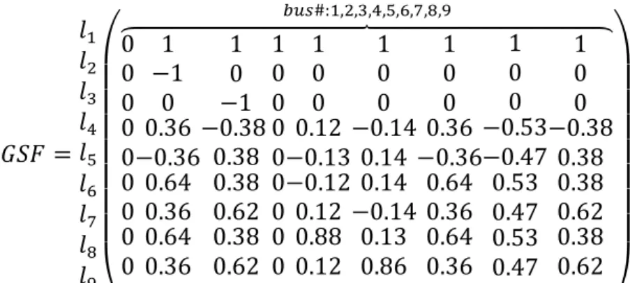
The next very important step is to calculate the Generation Shift Factors. This matrix contains network distribution factors. GSF represents the amount of real power flowing in the line ik as a result of injection of 1MW at bus j. Notation “(ik)j” represents elements of GSF matrix in the row corresponding to transmission line ik (from bus i to bus k) and in the column corresponding to bus j. The matrix is obtain as follows:

GSF(ik)j =

, ,

,

If j corresponding to the slack bus GSF(ik)j = 0

GSF1,1 = = 0 , bus 1 is a slack GSF1,2 = = , , = - 0,6 GSF1,3 = = , , = - 0,28 GSF2,1 = = 0, bus 1 is a slack GSF2,2 = = , , = - 0,39 GSF2,3 = = , , = - 0,72 GSF3,1= = 0, bus 1 is a slack GSF3,2= = , , , = 0,4 GSF3,3 = = , , , = - 0,29

As a result we get GSF =

0 −0,6 − 0,28 0 −0,39 − 0,72 0 0,4 − 0,29

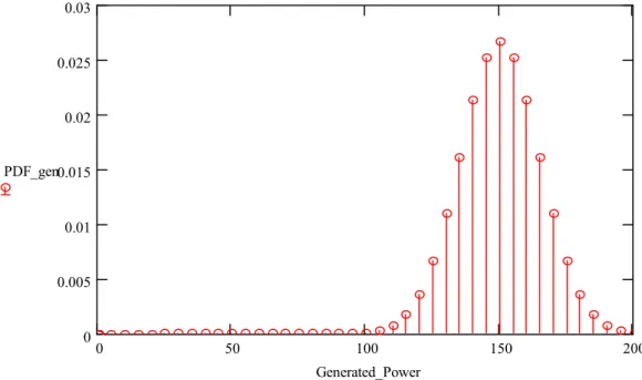
GSF is the basis of further calculations but it is a deterministic quantity and the generation at bus 2 is described by a normal distribution function N(150,10%). Thus all the parameters have to be discretized. In this example, random generation at bus 2 is discretized to the following probability sequence: the sequence interval is chosen to be 0.1MW and discretization window to be [µ -3σ, µ +3σ] (because 99,7% of values drawn from a normal distribution are within three standard deviations). Since generation at bus 2 is normally distributed with σ=10%, the selected window is [105MW, 195MW] based on the information in Table 2.3. The upper bound of 195MW and sequence interval of 0.1MW set the length of the sequence to be 1950, i.e. there will be 1950 observations in the probability sequence for this random generation. Since the lower bound of 105MW is µ-3σ, the probabilities of any sequence values beyond this lower bound are so small that they can be safely assumed to be zero. Fig. 2.2. plots the discrete probability sequence representing generation at bus 2.

FIG. 2.3 PROBABILITY SEQUENCE OF GENERATION AT BUS 2

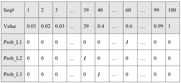
Discretization of a constant, i.e. generation shift factor, in this example, is straightforward: the probabilities of all sequence values are zero except the one is equal to the constant. This probability equals 1. Table 2.5 summarizes the example

0 50 100 150 200 0 0.005 0.01 0.015 0.02 0.025 0.03 PDF_gen Generated_Power

showing discretization of the generation shift factors of bus 2 for transmission lines 1, 2, 3, which equal 0.6, 0.39, and 0.4, respectively. Since the generation shift factors range in values from 0 to 1, if the sequence interval is chosen to be 0.01, the maximal sequence length will be 100. The sequences of aforementioned three shift factors are shown in Table 2.5. The first row lists the sequence number, while in the second row contains the discrete sequence values. Probability sequences corresponding to shift factors for line 1, 2 and 3 are shown in the third, the forth, and the fifth rows, respectively. Since shift factor is deterministic, the probability equals one when the sequence value equals to the corresponding shift factor, which is highlighted in bold italic font in Table 2.5, while all others are equal to zero. For example, in the sequence of shift factor for line 1, the coefficient at sequence number 60 is one, meaning the probability for sequence value to be equal to the corresponding shift factor, 0.6, is one.

TABLE 2.5 SEQUENCES OF GENERATION SHIFT FACTOR OF BUS 2 FOR LINE 1, 4 AND 6

Seq# 1 2 3 … 39 40 … 60 … 99 100

Value 0.01 0.02 0.03 … 39 0.4 … 0.6 … 0.99 1

Prob_L1 0 0 0 … 0 0 … 1 … 0 0

Prob_L2 0 0 0 … 1 0 … 0 … 0 0

Prob_L3 0 0 0 … 0 1 … 0 … 0 0

Once all the random and deterministic inputs are discretized, the distributions of the line flows can be calculated through the sequence operations, i.e., SMO, ATC and STC. SMO will be used to compute the line flow contributions of the individual net injected power at each bus. The contribution of random generation at bus 2 on:

a) transmission line 1 can be found through sequence multiplication between the probability sequence shown in Fig. 2.3 and the deterministic sequence of generation shift factor shown in the third row in Table 2.5:

b) transmission line 2 can be found through sequence multiplication between the probability sequence shown in Fig. 2.3 and the deterministic sequence of generation shift factor shown in the fourth row in Table 2.5,

B2_on_L2 = SMO(PDF_gen, Prob_L2)

c) transmission line 3 can be found through sequence multiplication between the probability sequence shown in Fig. 2.3 and the deterministic sequence of generation shift factor shown in the fifth row in Table 2.5.

B2_on_L3 = SMO(PDF_gen, Prob_L3)

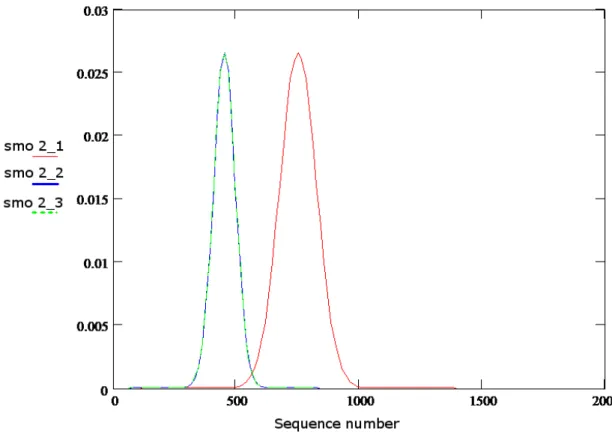
The results are presented below :

FIG. 2.4 CONTRIBUTION OF THE RANDOM GENERATION AT BUS 2 TO THE FLOWS IN LINES 1, 2 AND 3

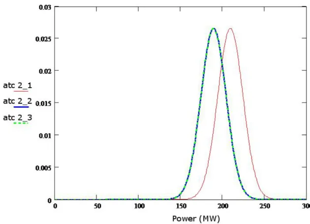
The total line flows on line x can be found by aggregating the contributions from the net injected powers in other buses with ATC or STC:

1) ATC on line 1, 2 and 3 2) STC on line 1,2 and 3

FIG. 2.5 THE TOTAL LINE FLOWS ON LINES CALCULATED USING ATC

3. COMPUTER PROGRAM FOR PLF CALCULATIONS

The program is written to make a proper calculations of Probabilistic Load Flow according to SOT method presented in chapter 2.6. Project is created in Fortran 90/95 environment. The program which is developed to work with the project is called “Compaq Visual Fortran 6”. To make code more readable it was divided into 9 parts. Each one is implemented as a different source file, as presented below:

- main.f90

- convolution.f90 (include 4 subroutine: ATC, STC, SMO calculation and discretization)

- matrices.f90 (in this section GSF matrix is calculated) - def_constant.f90 (all parameters are defined in that section) - def_variables.f90 (variables are defined here)

- def_types.f90 (all types of input variables are defined here) - read_input.f90 (this part corresponds to reading input files) - output.f90 (corresponds to creating output files and print results) - res_errors.f90 (contains the list of errors)

As an input input.raw and rndgn.txt are read. To simplify using the program input files should be located in INPUT_AND_OUTPUT_FILES folder. The format of input files was imposed. It is the most common format in energetic companies used to describing network configuration in power systems. Description of the input files is given in Section 3.1.1.1.

It was added extra code to check/debug the correctness of algorithms and calculations: e.g. all calculated matrix can be printed. It helped to check if code and calculations are proper. User can turn on the debugging process. In order to do this, set up parameter DEBUG as a true. In that case fort.10 file is created. In that file all calculated matrix are saved. The following matrices are saved during the debug:

- Admittance matrix (Matrix Y)

- Admittance matrix with removed one row and one column (Matrix Y1) - Inverted admittance matrix Y1 (Matrix Y1-1)

- Fully inverted matrix Y – Y1 with added a row and a column containing zeros (Matrix Y_1)

- Generation Shift Factor Matrix (Matrix GSF)

Another important issue is to create escape in case of error and print the reason of exit. In case of error, information about fault is printed on the screen. List of errors which can be recognised is presented below:

- Unable to read input file - Problems with input file - Input data file does not exist - Problems with reading input data - Bus Data are missing

- Load Data are missing - Generator Data are missing - Branch Data are missing - Read Bus Data Error - Read Load Data Error - Read Generator Data Error - Read Branch Data Error

As a final product program creates 3 outputs files SMO_out, ATC_out and STC_out in INPUT_AND_OUTPUT_FILES folder.

3.1.1. DATA PREPARATION

The program reads input file and saves the network configuration and random generation parameters in appropriate variables. From the input data a matrix of line impedance is created and subsequently a matrix of admittance. The admittance matrix is then used for creating generation shift factor. The program reads input data in the

subroutine read_input_data() and creates the matrices of impedance, admittance and generation shift factor in the subroutine Calculate_GSF().

3.1.1.1. INPUTS

Program reads data from two files. Information about network configuration (buses, generation, load, branches) from the first one called “input.raw” and information about random generation from the second file called “rndgn.txt”.

Example of the “input.raw” for 6 buses network

0 100.00 / PSS/E-26 RAW 1 'Bus_No_1' 138.000 3 0.000 0.000 1 1 1.05000 0.00 1 2 'Bus_No_2' 138.000 2 0.000 0.000 1 1 1.05000 8.60 1 3 'Bus_No_3' 138.000 1 0.000 0.000 1 1 1.02130 -4.32 1 4 'Bus_No_4' 138.000 1 0.000 0.000 1 1 1.01460 -3.64 1 5 'Bus_No_5' 138.000 1 0.000 0.000 1 1 1.01290 -5.31 1 6 'Bus_No_6' 138.000 1 0.000 0.000 1 1 1.00810 -6.66 1 0 / END OF BUS DATA, BEGIN LOAD DATA

2 01 1 1 1 20.0000 0.000 0.000 0.000 0.000 0.000 1 3 02 1 1 1 85.0000 0.000 0.000 0.000 0.000 0.000 1 4 03 1 1 1 40.0000 0.000 0.000 0.000 0.000 0.000 1 5 04 1 1 1 20.0000 0.000 0.000 0.000 0.000 0.000 1 6 05 1 1 1 20.0000 0.000 0.000 0.000 0.000 0.000 1 0 / END OF LOAD DATA, BEGIN GENERATOR DATA

1 01 60.700 0.000 50. -40. 1.05000 0 100.000 0.00000 1.00000 0.00000 0.00000 1.00000 1 100.0 110.000 0.000 1 1.0000 0 0.0000 0 0.0000 0 0.0000

2 02 130.000 0.000 75. -40. 1.05000 0 100.000 0.00000 1.00000 0.00000 0.00000 1.00000 1 100.0 130.000 80.000 1 1.0000 0 0.0000 0 0.0000 0 0.0000

0 / END OF GENERATOR DATA, BEGIN BRANCH DATA

1 3 1 0.0342 0.18 0.0212 85.00 85.00 0.00 0.00000 0.000 0.00000 0.00000 0.00000 0.00000 1 1.0 1 1.0000 0 0.0000 0 0.0000 0 0.0000

2 4 1 0.1140 0.60 0.0704 71.00 71.00 0.00 0.00000 0.000 0.00000 0.00000 0.00000 0.00000 1 1.0 1 1.0000 0 0.0000 0 0.0000 0 0.0000

1 2 1 0.0912 0.48 0.0564 71.00 71.00 0.00 0.00000 0.000 0.00000 0.00000 0.00000 0.00000 1 1.0 1 1.0000 0 0.0000 0 0.0000 0 0.0000 3 4 1 0.0228 0.12 0.0142 71.00 71.00 0.00 0.00000 0.000 0.00000 0.00000 0.00000 0.00000 1 1.0 1 1.0000 0 0.0000 0 0.0000 0 0.0000 3 5 1 0.0228 0.12 0.0142 71.00 71.00 0.00 0.00000 0.000 0.00000 0.00000 0.00000 0.00000 1 1.0 1 1.0000 0 0.0000 0 0.0000 0 0.0000 1 3 2 0.0342 0.18 0.0212 85.00 85.00 0.00 0.00000 0.000 0.00000 0.00000 0.00000 0.00000 1 1.0 1 1.0000 0 0.0000 0 0.0000 0 0.0000 2 4 2 0.1140 0.60 0.0704 71.00 71.00 0.00 0.00000 0.000 0.00000 0.00000 0.00000 0.00000 1 1.0 1 1.0000 0 0.0000 0 0.0000 0 0.0000 4 5 1 0.0228 0.12 0.0142 71.00 71.00 0.00 0.00000 0.000 0.00000 0.00000 0.00000 0.00000 1 1.0 1 1.0000 0 0.0000 0 0.0000 0 0.0000 5 6 1 0.0228 0.12 0.0142 71.00 71.00 0.00 0.00000 0.000 0.00000 0.00000 0.00000 0.00000 1 1.0 1 1.0000 0 0.0000 0 0.0000 0 0.0000

0 / END BRANCH DATA, BEGIN TRANSFORMER ADJUSTMENT DATA

0 / END TRANSFORMER ADJUSTMENT DATA, BEGIN AREA INTECHANGE DATA 0 / END OF AREA INTECHANGE DATA, BEGIN TWO-TERMINAL DC DATA 0 / END OF TWO-TERMINAL DC DATA, BEGIN SWITCHED SHUNT DATA 0 / END OF SWITCHED SHUNT DATA, BEGIN TRANS. IMP. CORR. TABLE DATA

0 / END OF TRANS. IMP. CORR. TABLE DATA, BEGIN MULTI-TERMINAL DC LINE DATA 0 / END OF MULTI-TERMINAL DC LINE DATA, BEGIN MULTI-SECTION LINE DATA 0 / END OF MULTI-SECTION LINE DATA, BEGIN ZONE DATA

0 / END OF ZONE DATA, BEGIN INTERAREA TRANSFER DATA 0 / END INTERAREA TRANSFER DATA, BEGIN OWNER DATA 0 / END OF OWNER DATA, BEGIN FACTS DEVICE DATA 0 / END OF FACTS DEVICE DATA, END OF CASE DATA

Important is that not all data are used but for future develop all are read to program.

Data which are used:

First section - BUS DATA – first column informs about number of the bus and fourth

column informs about type of the bus (If the value is 1 the bus is a load, if the value is 2 the bus is a generation and it the value is 3 the bus is a slack).

Second section – LOAD DATA – first column informs about number of bus, sixth column informs about value of the load.

Third section – GENERATION DATA – first column informs about number of bus, third column informs about value of the generation.

Fourth section – BRANCH DATA – fifth column inform about reactance between buses from first and second column.

Example of the “rndgn.txt” is presented below:

#first random generation is defined as a continuous normal distr. at bus 2, mean=163 and stdev=16.3

2 2 0 163.00000 16.30000 0.0 0.0 0.0

#second random generation is defined as a discrete distribution at the bus 3, 11 following lines define the distribution

3 1 11 0.0 0.00000 0.0 0.0 0.0 113.00000 123.00000 133.00000 143.00000 153.00000 163.00000 173.00000 183.00000 193.00000 203.00000 213.00000

It is formatted according to the following pattern:

1) Lines starting with # sign are considered as comments and not read

2) First number (integer) in the line defines the number of a bus at which random generation occurs

3) Second number (integer) defines type of the distribution: 1 – discrete (user must provide additional information for this kind of distribution), 2 – Normal distribution, 3 – Weibull distribution

4) Central value (or mean): mandatory for Normal distribution, ignored for discrete and optional for Weibull distribution

5) Standard deviation: mandatory for Normal distribution, ignored for discrete and optional for Weibull distribution

6) Scale parameter: mandatory for Weibull, ignored otherwise

7) Shape parameter: mandatory for Weibull (0 for 1-parameter Weibull distribution), ignored otherwise

8) Location parameter: mandatory for Weibull (0 for 1- or 2-parameter Weibull distribution), ignored otherwise

3.1.2. DISCRETIZATION

As previously discussed, all inputs are discretized, including both random variables and constants. If an input variable is already discrete it does not have to be processed but if it is a continuous type the recommended initial step length of sequence is determined in such a way that the step length is 1/10th of the standard deviation of the underlying input random variable. A separate subroutine named discretization() was created to achieve this task.

3.1.3. SEQUENCE OPERATION

In order to perform sequence operation three subroutines were created. Their names correspond to the operation they performed, thus

a) subroutine ATC(rows_A, mx_A, rows_B, mx_B, rows_C, mx_C_out) performs addition type convolution of two vectors mx_A and mx_B returning vector mx_C_out as the result;

b) subroutine STC(rows_A, mx_A, rows_B, mx_B, rows_C, mx_C_out) performs subtraction type convolution of two vectors mx_A and mx_B returning vector mx_C_out as the result;

c) subroutine SMO(rows_A, mx_A, rows_B, mx_B, rows_C, mx_C_out) performs sequence multiplication operation on two vectors mx_A and mx_B returning vector mx_C_out as the result.

3.2. TESTS ON 9-BUS SYSTEM

The studies presented below are based on the standard IEEE 9-bus system [15]. Data obtained as a result of program’s work in debugging process are compared with manual calculations for the same network to check if the program is working in proper way.

3.2.1. DATA AND MANUAL CALCULATIONS

Under consideration are three generators located at bus 1, bus 2 and bus3, and three loads located at bus 5, bus 6 and bus 8. Bus 1 is assigned to be the slack. The topology is shown in Fig 3.1 below. The line parameters are included in Table 3.1. The matrix of generation shift factors can be easily formulated based on the information in Table 3.1 and Fig 3.1, as shown below. To ease the illustration, only generation at bus 2 is considered as variable resource, and assumed to be described by a normal distribution. Generations at other buses as well as all the loads are assumed to be deterministic. The information is summarized in Table 3.2.

FIG. 3.1 THE 9-BUS SYSTEM OF THE EXAMPLE = ⎝ ⎜ ⎜ ⎜ ⎜ ⎜ ⎜ ⎜ ⎛0 0 0 0 0 0 0 0 0 1 −1 0 0.36 −0.36 0.64 0.36 0.64 0.36 1 0 −1 −0.38 0.38 0.38 0.62 0.38 0.62 1 0 0 0 0 0 0 0 0 1 0 0 0.12 −0.13 −0.12 0.12 0.88 0.12 1 0 0 −0.14 0.14 0.14 −0.14 0.13 0.86 1 0 0 0.36 −0.36 0.64 0.36 0.64 0.36 1 0 0 −0.53 −0.47 0.53 0.47 0.53 0.47 1 0 0 −0.38 0.38 0.38 0.62 0.38 0.62 #: , , , , , , , , ⎠ ⎟ ⎟ ⎟ ⎟ ⎟ ⎟ ⎟ ⎞

GENERATION SHIFT FACTOR FOR THE SYSTEM FROM FIG 3.1

As discussed earlier, all inputs need to be discretized, including both random variables and constants, prior to sequence operation: random variables need to be converted to probability sequences, and relevant constants need to be converted to deterministic sequences.

TABLE 3.1 IMPEDANCE OF THE TRANSMISSION SYSTEM

Line From Bus To Bus R [p.u.] X [p.u.]

1 4 1 0 0.0576

2 7 2 0 0.0625

4 7 8 0.0085 0.072 5 9 8 0.0119 0.1008 6 7 5 0.032 0.161 7 9 6 0.039 0.17 8 5 4 0.01 0.085 9 6 4 0.017 0.092

TABLE 3.2 GENERATION AND LOAD INFORMATION

Bus# Type P [MW] Input Type

1 Slack 71.63 Non-random

2 Gen. 163 Random, Normal Distribution

µ=163 [MW], σ=10% 3 Gen. 85 Non-random 4 Load 0 Non-random 5 Load 125 Non-random 6 Load 90 Non-random 7 Load 0 Non-random 8 Load 100 Non-random 9 Load 0 Non-random

In this example, random generation at bus 2 is discretized to the following probability sequence: the sequence interval is chosen to be 0.1MW and discretization window to be [µ -3σ, µ +3σ]. Since generation at bus 2 is normally distributed with σ=10%, the selected window is [114MW, 212MW] based on the information in Table 3.2. The upper bound of 212MW and sequence interval of 0.1MW set the length of the sequence to be 2120, i.e. there will be 2120 observations in the probability sequence for this random generation. Since the lower bound of 114MWis µ-3σ, the probabilities of any sequence values beyond this lower bound are so small that they can be safely assumed to be zero. Fig 3.2 plots the discrete probability sequence representing generation at bus 2. The choices for sequence interval and window width depend on user’s preference to the trade-off between the accuracy and size of the sequence. Discretization of a constant, i.e. generation shift factor, in this example, is straight forward :the probabilities of all sequence values are zero except the one is equal to the constant. This probability equals 1. Table 3.3 shows the example showing discretization of generation shift factors of bus 2 for transmission line1,4,6, which equal 1, 0.36, and 0.64 respectively. Since the generation shift factors range in values from 0 to 1, if the sequence interval is chosen to be 0.01, the maximal sequence length will be 100. The sequences of aforementioned four shift factors are shown in Table 3.3. The first row lists the sequence number, while in the second row are the discrete sequence values. Probability sequences corresponding to shift factors for line 1, 4 and 6 are shown in the third, the forth, and the fifth row, respectively. Since shift factor is deterministic, the probability equals one when the sequence value equals to the corresponding shift factor, which is highlighted in bold italic font in Table 3.3, while all others are equal to zero. For example, in the sequence of shift factor for line 4, the coefficient at sequence number 36 is one, meaning the probability for sequence value to be equal to the corresponding shift factor, 0.36, is one.

TABLE 3.3 SEQUENCES OF GENERATION SHIFT FACTOR OF BUS 2 FOR LINE 1, 4 AND 6 Seq# 1 2 3 4 … 36 … 64 … 99 100 Value 0.01 0.02 0.03 0.04 … 0.36 … 0.64 … 0.099 1 Prob_L1 0 0 0 0 … 0 … 0 … 0 1 Prob_L4 0 0 0 0 … 1 … 0 … 0 0 Prob_L6 0 0 0 0 … 0 … 1 … 0 0

Once all the random and deterministic inputs are discretized, the distributions of line flows can be calculated through sequence operations, i.e., SMO, ATC and STC. SMO will be used to compute the line flow contributions of the individual net injected power at each bus. For example, the contribution of random generation at bus 2 on transmission line 6 can be found through sequence multiplication between the probability sequence shown in Fig 3.2 and the deterministic sequence of generation shift factor shown in the fifth row in Table 3.3.

FIG. 3.2 PROBABILITY SEQUENCE OF GENERATION AT BUS 2

0 50 100 150 200 250 0 0.005 0.01 0.015 0.02 0.025 Generated power [MW] P ro b ab il it y [ p .u .] gen_probi Pi

The total line flows on line 6 can be found by aggregating the contributions from the net injected powers in other buses with ATC or STC. As discussed earlier, this probability sequence can be converted to probability distribution.

3.2.2. DEBUG PROCESS

During coding process used some additional function to debugging. For this purpose, matrixes are printed to standard fortran file called “fort.10” the result is printed if the parameter “DEBUG” is set as true ( we can find this parameter in “def_constants” section)

The content of this file for 9 bus network is presented below:

Matrix X (impedance) : 0.000 0.000 0.000 0.058 0.000 0.000 0.000 0.000 0.000 0.000 0.000 0.000 0.000 0.000 0.000 0.063 0.000 0.000 0.000 0.000 0.000 0.000 0.000 0.000 0.000 0.000 0.059 0.058 0.000 0.000 0.000 0.085 0.092 0.000 0.000 0.000 0.000 0.000 0.000 0.085 0.000 0.000 0.161 0.000 0.000 0.000 0.000 0.000 0.092 0.000 0.000 0.000 0.000 0.170 0.000 0.063 0.000 0.000 0.161 0.000 0.000 0.072 0.000 0.000 0.000 0.000 0.000 0.000 0.000 0.072 0.000 0.101 0.000 0.000 0.059 0.000 0.000 0.170 0.000 0.101 0.000

Matrix Y (admittance): 17.241 0.000 0.000 -17.241 0.000 0.000 0.000 0.000 0.000 0.000 15.873 0.000 0.000 0.000 0.000 -15.873 0.000 0.000 0.000 0.000 16.949 0.000 0.000 0.000 0.000 0.000 -16.949 -17.241 0.000 0.000 39.876 -11.765 -10.870 0.000 0.000 0.000 0.000 0.000 0.000 -11.765 17.976 0.000 -6.211 0.000 0.000 0.000 0.000 0.000 -10.870 0.000 16.752 0.000 0.000 -5.882 0.000 -15.873 0.000 0.000 -6.211 0.000 35.973 -13.889 0.000 0.000 0.000 0.000 0.000 0.000 0.000 -13.889 23.790 -9.901 0.000 0.000 -16.949 0.000 0.000 -5.882 0.000 -9.901 32.732

Matrix Y1 (admittance matrix with removed one row and one column):

15.873 0.000 0.000 0.000 0.000 -15.873 0.000 0.000 0.000 16.949 0.000 0.000 0.000 0.000 0.000 -16.949 0.000 0.000 39.876 -11.765 -10.870 0.000 0.000 0.000 0.000 0.000 -11.765 17.976 0.000 -6.211 0.000 0.000 0.000 0.000 -10.870 0.000 16.752 0.000 0.000 -5.882 -15.873 0.000 0.000 -6.211 0.000 35.973 -13.889 0.000 0.000 0.000 0.000 0.000 0.000 -13.889 23.790 -9.901 0.000 -16.949 0.000 0.000 -5.882 0.000 -9.901 32.732

Matrix Y1_1 (inverted admittance matrix Y1): 0.278 0.153 0.058 0.112 0.091 0.215 0.189 0.153 0.153 0.278 0.058 0.091 0.115 0.153 0.180 0.219 0.058 0.058 0.058 0.058 0.058 0.058 0.058 0.058 0.112 0.091 0.058 0.132 0.069 0.112 0.103 0.091 0.091 0.115 0.058 0.069 0.138 0.091 0.101 0.115 0.215 0.153 0.058 0.112 0.091 0.215 0.189 0.153 0.189 0.180 0.058 0.103 0.101 0.189 0.228 0.180 0.153 0.219 0.058 0.091 0.115 0.153 0.180 0.219

Matrix Y_1 (fully inverted matrix Y – Y1 with added a row and a column containing zeros): 0.000 0.000 0.000 0.000 0.000 0.000 0.000 0.000 0.000 0.000 0.278 0.153 0.058 0.112 0.091 0.215 0.189 0.153 0.000 0.153 0.278 0.058 0.091 0.115 0.153 0.180 0.219 0.000 0.058 0.058 0.058 0.058 0.058 0.058 0.058 0.058 0.000 0.112 0.091 0.058 0.132 0.069 0.112 0.103 0.091 0.000 0.091 0.115 0.058 0.069 0.138 0.091 0.101 0.115 0.000 0.215 0.153 0.058 0.112 0.091 0.215 0.189 0.153 0.000 0.189 0.180 0.058 0.103 0.101 0.189 0.228 0.180 0.000 0.153 0.219 0.058 0.091 0.115 0.153 0.180 0.219

Matrix GSF: 0.000 1.000 1.000 1.000 1.000 1.000 1.000 1.000 1.000 0.000 -1.000 0.000 0.000 0.000 0.000 0.000 0.000 0.000 0.000 0.000 -1.000 0.000 0.000 0.000 0.000 0.000 0.000 0.000 0.361 -0.385 0.000 0.125 -0.135 0.361 -0.533 -0.385 0.000 -0.361 0.385 0.000 -0.125 0.135 -0.361 -0.467 0.385 0.000 0.639 0.385 0.000 -0.125 0.135 0.639 0.533 0.385 0.000 0.361 0.615 0.000 0.125 -0.135 0.361 0.467 0.615 0.000 0.639 0.385 0.000 0.875 0.135 0.639 0.533 0.385 0.000 0.361 0.615 0.000 0.125 0.865 0.361 0.467 0.615

The test and debug process covered the following steps in the process of solving problem:

Step Purpose Methodology Result

Reading input data

To check whether all the parameters are correctly

read

After reading the variables were printed out and the results were compared against the

input data file.

Positive

Matrix of line impedance

To check whether the matrix of line impedances

is properly created

The matrix of impedances was compared element by element against the known network diagram and the matrix from the

computational example (Table 3.1).

Positive

Matrix of line admittance

To check whether the matrix of line admittances

The matrix of impedances was only checked whether it is created and the

is properly created elements have reasonable values. Attention was also paid to the errors and avoiding

them using sanity check in vulnerable points (i.e. dividing by zero).

Generation shift factor

GSF

To check whether the GSF is properly created

Calculated GSF for 9-bus system was compared element by element against the

one from the computational example.

Positive

Discretization

To check whether the discrete values correspond to the continuous function

The results of discretization were

compared against the manual calculations. Positive

Sequence operation: ATC, STC

and SMO

To check whether the sequence operators work

properly

The subroutines ATC, STC and SMO were tested in two steps. The purpose of the first

step was to obtain the same results as presented in the Table 2.2. The purpose of

the second step was to obtain the same results for the 9-bus system as in the

example and in Fig. 3.2.

Positive

3.2.3. OUTPUT

As a result, the program generated 3 txt files: ATC_out, STC_out and SMO_out.

In SMO_out the contribution of a random generation at each generation bus is described.

In ATC_out and STC_out the contribution of total line flow and generation at each generation bus on all lines is described.

3.3. 24-BUS IEEE TEST SYSTEM

The largest tested network has 24 buses. The system is an IEEE 24-bus reliability test system based on [14] with the diagram shown below.

The test on this system was performed using data presented in Appendix A. Appendix B contains intermediate results which may be useful for any further comparison, testing or debugging purpose. The testing procedure involved the following analysis:

 the line flow contributions of the individual net injected power at each bus (SMO), and

 the total lines flow influence on each line (ATC).

Environment used during test:

 computer's specification: Dell inspiron 1545  operating system: Windows XP

The computation time: 8.7 sec

Figures 3.4 – 3.6 show the results for the chosen lines and two generating buses.

FIG. 3.4 THE CONTRIBUTION OF RANDOM GENERATION AT BUSES 2 AND 15 ON THE FLOWS IN TRANSMISSION LINE 6

FIG. 3.5 THE CONTRIBUTION OF TOTAL LINE FLOWS AND GENERATION AT BUS 2 ON LINES 1-7