T. G. Ritto
[email protected] Department of Mechanical Engineering Federal University of Rio de Janeiro (UFRJ), BrazilRubens Sampaio
[email protected] Department of Mechanical Engineering PUC-Rio, BrazilF. A. Rochinha
[email protected] Department of Mechanical Engineering Federal University of Rio de Janeiro (UFRJ), BrazilModel Uncertainties of Flexible
Structures Vibrations Induced by Internal
Flows
In many situations analysts use incomplete models to design a system, or to make decisions. These models are incomplete due to unmodeled phenomena, which means that some features are not included in the model (either because it was not previously thought about or because it would be too expensive to include). These uncertainties related to the model are difficult to take into account. In this paper, the nonparametric probabilistic approach is used to investigate model uncertainties in the problem of structures excited by internal flow. A reference model is constructed, where an Euler-Bernoulli beam is used to model the structure, and the fluid is added to the model by means of a constant mass, damping and stiffness. Then, an incomplete model of the reference model is considered. In it the influence of the fluid stiffness is not taken into account, hence, the uncertainty is related to this unmodeled feature (fluid stiffness). The incomplete model is then used together with the nonparametric probabilistic approach to infer the behavior of the reference model. Besides, a procedure is proposed to calibrate the dispersion parameter of the probabilistic model.
Keywords: fluid-structure interaction, stochastic dynamical model, inverse stochastic problem, model uncertainties
Introduction
The application analyzed in this paper is the flexible-structure vibrations induced by internal flows. The dynamics of structures with internal axial flow has many technological applications, e.g., drill-strings (Ritto et al. (2009)) heat-exchanger tubes, microscale resonators (Rinaldi et al. (2010)), nuclear fuel elements, towed flexible cylinders for water transportation, etc. In the present analysis the fluid-structure interaction is modeled as done by Paidoussis (1998), where the Euler-Bernoulli beam theory is used to model the structure, and the system is discretized by means of the finite element method.
Uncertainties related to structures excited by internal flow have not got the attention it deserves. Curling and Paidoussis (2003) investigate cylinders subjected to turbulent axial flow, and analytical approximations for the lateral fluid forcing functions have been presented, where these excitations are random. For a general perspective on modeling uncertainties, see Ayyub and Klir (2006) and Caers (2011).
The interest of the present investigation is on model uncertainties, i.e., modeling errors due to incomplete information and unmodeled phenomena. For the present analysis, a reference model is constructed, and a computational incomplete model is considered, where the influence of the fluid stiffness is not taken into account, i.e., the unmodeled phenomenon is the fluid stiffness (which is not included in the incomplete model). It should be noted that this choice is arbitrary, the incomplete model considered could be another one, e.g., the fluid mass, or the damping, etc. The question that arises is the following: is there a strategy to generate good predictions using the incomplete model? When analyzing complex systems, incomplete models are always used to predict the response of the real system. By controlling the model uncertainty, as proposed in this work, it is possible to know exactly what the unmodeled phenomenon is and, hopefully, to gain some confidence in using incomplete models.
It should be noted that a careful analysis of uncertainties for the system analyzed in the present work will be the subject of a future work. For instance, if the stiffness is uncertain it is likely that the
Paper received 14 January 2011. Paper accepted 24 May 2011.
Technical Editor: Marcelo Trindade
inertia and damping of the structure are also uncertain, since there is a correlation among these quantities. The present paper focuses the analysis on only one uncertain aspect, such that the modeling error can be controlled and better analyzed.
There are few strategies found in the literature to cope with model uncertainties. There is the info-gap model uncertainty (Ben-Haim (2006)), where a non-probabilistic strategy is pursued and nested sets are considered. There is the nonparametric probabilistic approach (Soize (2000)), where a probabilistic strategy is pursued and the random matrix theory is applied (Mehta (1991)). There is the strategy found in Beck and Katafygiotis (1998), where the output prediction errors include model uncertainties (output prediction errors is the difference between numerical and real system outputs). Recently, model uncertainty is being called model form uncertainty. Roy and Oberkampf (2011) take into account model form uncertainty appending an area validation metric to the sides of the p-box (ensemble of cumulative density functions).
The nonparametric probabilistic approach (Soize (2000)) is appealing, since it is the only strategy implemented at the operator level of the model. Therefore, in the present work it will be used to model uncertainties. The procedure adopted in this paper is similar to the one followed by Ritto et al. (2008), where the nonparametric probabilistic approach was employed to the problem of a beam with uncertainty on the boundary conditions. However, the type of uncertainty analyzed now is very different and here a calibration procedure is proposed (inverse stochastic problem).
The main contributions of this paper are the following: 1) investigation of model uncertainties in structures excited by internal flow using the nonparametric probabilistic approach, 2) proposition of a calibration procedure for the dispersion parameter of the probabilistic model, and 3) benchmark for other analyses related to model uncertainties. Concerning point three, it should be remarked that the simple system considered in the present work is well suited for comparisons of different strategies for modeling uncertainties within the model.
constructed with the normal modes of the structure, is presented. The stochastic model (nonparametric probabilistic approach) is quickly reviewed in the third section, and the resulting stochastic system is shown in the fourth section. In the fifth section, the calibration procedure is explained and the stochastic system is analyzed. Finally, in the sixth section, the concluding remarks are made.
Nomenclature
E = Young Modulus, Pa F = external force, N/m L = length, m
I = area moment of inertia, m4
m = mass per unit length of the structure, kg/m Mf = mass per unit length of the fluid, kg/m U = fluid velocity, m/s
u = dimensionless fluid velocity v = transversal displacement, m
δ = dispersion parameter v = displacement vector, m, rad f = force vector, N, N.m N = shape function vector [M] = mass matrix [Mr] = reduced mass matrix [C] = damping matrix [Cr] = reduced damping matrix [K] = stiffness matrix [Kr] = reduced stiffness matrix [Kr] = random reduced stiffness matrix [G] = random germ matrix
[H] = matrix of the frequency response functions
Greek Symbols
ωi = i-th natural frequency [Φ] = normal modes matrix
Deterministic System
Figure 1 sketches the system considered in the analysis.
Figure 1. Sketch of the system considered in the analysis (the arrow represents the internal fluid flow).
Using the Euler-Bernoulli beam theory, the partial differential equation governing the dynamics of the structure is written as:
m∂
2v(x,t)
∂t2 +EI
∂4v(x,t)
∂x4 =F(x,t) x∈[0,L],t∈[0,T], (1)
wherevis the transversal displacement,Lis the length of the beam, mis the mass per unit length,Eis the elasticity modulus,Iis the area moment of inertia andFis the external force. If the fluid (Paidoussis (1998)) is included in the model, the governing equation is:
(m+Mf)∂ 2v
∂t2+2MfU
∂2v
∂x∂t+MfU2∂ 2v
∂x2+EI
∂4v
∂x4=F, (2)
whereMf is the fluid mass per unit length andUis the constant axial velocity of the fluid. Using dimensionless variables, we can write:
∂2η
∂τ2+2β
1/2u ∂2η
∂ζ∂τ+u 2∂2η
∂ζ2+
∂4η
∂ζ4 = f, (3)
where the dimensionless quantities are:
τ=t
EI (m+Mf)L4
1/2
, f=FL
2
EI.
ζ= x
L, η=
v L,
β= Mf
m+Mf
, u=U L
Mf EI
1/2
,
(4)
MakingMf =0, we get the dimensionless form of Eq. (1). Let η=ηˆexp(iωτ)andf=fˆexp(iωτ), in whichωis the dimensionless
frequency, ω=ωrad (m+Mf)L 4
EI
!1/2
, ωrad is the frequency in
rad/s andi=√−1. Substitutingη=ηˆexp(iωτ)and f=fˆexp(iωτ) in Eq.(3) leads to:
−ω2ηˆ+iω2β1/2u∂ηˆ ∂ζ+u
2∂2ηˆ
∂ζ2+
∂4ηˆ
∂ζ4 =fˆ. (5)
The partial differential equation, Eq. (5), is discretized by means of the finite element method: ˆη(e)(ξ,ω) =N(ξ)vˆ(e)(ω), in which Nare the shape functions (Hermitian functions), ξ is the element coordinate, and ˆv(e)is the vector with the element displacements.
After assembling the element matrices, the discretized system is given by:
−ω2[M]ˆv(ω) +iω[C]ˆv(ω) + ([Kb] + [Kf])v(ˆ ω) =ˆf(ω), (6) where[M],[C],[Kb]and[Kf]∈Rm×mare the mass, damping and stiffness matrices (related to the bending and to the fluid), ˆv(ω)
∈Cm is the response vector and ˆf(ω) ∈Cm is the force vector. Matrices[M]and[Kb]are symmetric positive definite, matrix [Kf] is symmetric negative definite and matrix [C] is not necessarily symmetric. Equation (6) can be written as
ˆ
v(ω) = [H(ω)]ˆf(ω), (7)
where[H(ω)] ∈Cm×m is the frequency response function (FRF), formally cast as:
[H(ω)] = (−ω2[M] +iω[C] + ([Kb] + [Kf]))−1. (8) Reduced-Order Model
probabilistic approach, because the full finite element matrices have topological zeros, which cannot be replaced by nonzero random variables, Soize (2000).
The basis generated by the normal modes associated conservative system ([C] =0) is used to construct the reduced-order model. It should be noted that these modes do not diagonalize the damping matrix.
The natural frequencies and the normal modes of the reference model are computed from the following generalized eigenvalue problem:
(−ω∗i2[M] + [Kb] + [Kf])φ∗i=0, (9)
whereω∗i is thei-th natural frequency,φ∗iis thei-th normal mode, and the matrix composed by the first normal modes is given by[Φ∗] = [φ∗1φ∗2...φ∗n]. Note that the reference model includes[Kf](fluid stiffness), which depends onu; therefore, for eachua different basis is generated. The reduced stiffness matrix of the reference model is written as
[Kr∗] = [Φ∗]T([Kb] + [Kf])[Φ∗]. (10)
As mentioned before, the unmodeled phenomenon is known to be the fluid stiffness, and the nonparametric probabilistic model (see next section) is going to be used together with the incomplete computational model. The natural frequencies and normal modes of the incomplete model are computed from the following generalized eigenvalue problem (which does not include[Kf]-fluid stiffness):
(−ω2i[M] + [Kb])φi=0, (11) whereωi is thei-th natural frequency,φiis thei-th normal mode, and the matrix composed by the normal modes is given by[Φ] = [φ1φ2...φn]. The reduced stiffness matrix of the incomplete model is written as
[Kr] = [Φ]T[Kb][Φ]. (12)
Now, let ˆv(ω) = [Φ]ˆq(ω), where[Φ]∈Rm×nis the matrix composed by the normal modes of the system and ˆq(ω)∈Cn. The reduced-order model of the incomplete system can be written as
ˆ
q(ω) = (−ω2[Mr] +iω[Cr] + [Kr])−1[Φ]Tˆf(ω). (13)
Thus, the system was reduced from dimensionmton(n<m). The reduced mass and damping matrices are constructed using[Φ]as done in Eq. (12). The reduced-order model of the reference system can be written as
ˆ
qre f(ω) = (−ω2[Mr∗] +iω[Cr∗] + [Kr∗])−1[Φ∗]Tˆf(ω), (14) where the reduced mass and damping matrices are constructed using [Φ∗]as done in Eq. (10). Hence, in physical coordinates, the response
of the reference model is given by ˆvre f(ω) = [Φ∗]ˆqre f(ω).
Stochastic Model
The nonparametric probabilistic approach (Soize (2000)) is used as a strategy to model the uncertainties related to the unmodeled physical phenomenon (fluid stiffness). Such an approach consists in constructing a stochastic model for the stiffness operator of the problem using intrinsic available information relative to it.
The idea of this probabilistic approach is based on the fact that even if all the parameters of the incomplete model are modeled as random variables, the experimental response can not be properly described, since there are unmodeled phenomena (which means that the incomplete model lacks important features of the behavior of the system). To overcome this problem, instead of modeling the parameters of the incomplete model as random variables, the reduced-order matrix of the system is modeled as a random matrix in such a way that a larger set of outcomes is achieved and, hopefully, the experimental response will be within the larger set. A simple two-degrees-of-freedom example showing the difference between parameter and model uncertainties using the nonparametric probabilistic approach can be found in Sampaio and Cataldo (2010).
The reduced random matrix is written as (note that the boldface is used for the random matrices)
[Kr] = [L]T[G][L], (15)
where [L]T[L] is the Cholesky decomposition of matrix [K r] (Eq. (12)), which does not include the fluid stiffness[Kf]. Without going into further details, the probability density function of the random matrix[G]can be constructed using the Maximum Entropy Principle (Jaynes (2003)) with the following available information:
1. Random matrix[G]is almost surely positive-definite,
2. E{[G]}= [I] , 3. E{||[G]−1||2
F}=c1,|c1|<+∞ ,
where [I] is the identity matrix, E{·} denotes the mathematical expectation and||[A]||F= (trace{[A][A]T})1/2denotes the Frobenius norm. The first available information says that [Kr] is positive-definite almost surely, which is important to guarantee the physical characteristics of the stiffness of the system; the second available information says that the mean value of[Kr]is equal to its nominal value[Kr], which means that we supposedly trust the nominal model (it should be noted that modeling the problem is a constructive process and should be approached step by step; the nominal model must be updated if it cannot be sufficiently trusted); and the third available information guarantees that the response of the system is a second order process (i.e., the response is bounded for bounded input).
The closed form expression of the probability density function of [G]is given by (Soize (2000))
p[G]([G]) =1M+
n(R)([G])CGdet([G])
(n+1)(1−δ2)
2δ2 ×
×exp
−n2+δ21tr([G]) ,
(16)
where det(·)is the determinant, tr(·)is the trace,M+n(R)is the set of real positive-definite matrices of dimensionn. The normalization constant is written as
CG=
(2π)−n(n−1)/4 n+1 2δ2
n(n+1)/(2δ2)
∏n
j=1Γ (n+1)/(2δ2) + (1−j)/2
where Γ(z) is the gamma function defined for z>0 by Γ(z) =
´+∞
0 t
z−1e−tdt. An important parameter used in the analysis is the dispersion parameterδof matrix[G], defined as:
δ=
1
nE{||[G]−[I]||
2 F}
12
, (18)
Asδincreases, the uncertainty of the stiffness also increases. Note that[Kf]depends on the dimensionless speedu. Therefore, ifu=0, then the incomplete model equals the reference model, andδ=0. For different values ofu,δshould be calibrated, as shown in the following section.
The stochastic system is written as:
ˆ
Q(ω) = (−ω2[Mr] +iω[Cr] + [Kr])−1[Φ]Tˆf(ω), (19) where ˆQ(ω)is the random response, which is random because[Kr] is random.
Calibration Procedure and Numerical Analysis
The beam is supported in both ends (i.e.,η=0 atζ=0 and at
ζ=1). It is discretized with 80 finite elements (m=160) and the reduced-order model is constructed withn=10. The frequency band analyzed is[0,30]Hz. The mass ratioβ=0.8 is fixed anduvaries from 0 to 3. For instance, for the configurationE=450×106 Pa,
di=4×10⁻²m,do=5×10⁻²m,ρ=250 kg/m3,ρf=1000 kg/m3, U=10 m/s, we haveβ=0.88 andu=1.24.
Deterministic response
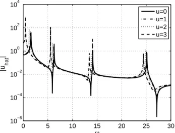
Figure 2 depicts the absolute value of the response |vˆ|of the deterministic system at ζ=0.3 for different flow velocities u=
{0,1,2,3}. It can be seen that the first natural frequency is the one that shifts the most (see Table 1).
0 5 10 15 20 25 30
10−6 10−4 10−2 100 102 104
ω
|u hat
|
u=0 u=1 u=2 u=3
Figure 2. Response in frequency of the deterministic system atζ=0.3for u={0,1,2,3}. Asuincreases the natural frequencies shift left.
Figure 3 shows the distance from the reference response as the dimensionless velocity increases. It shows how the two deterministic models get apart asuincreases. The distancedistis measured by:
dist(u) =100 nω
nω
∑
j=1
||vˆre f(ωj,u)−v(ˆ ωj)||
||v(ˆ ωj,u)||
, (20)
in which ˆvre f is the response of the reference model (stiffness matrix given by Eq. (12)) and ˆvis the response of the incomplete model using stiffness matrix given by Eq. (10). The frequency domain is discretized innω(=1500) frequencies, and|| · ||is the L2-norm.
0 0.5 1 1.5 2 2.5 3
0 50 100 150
u
dist (%)
Figure 3. Percent error as a function of the flow velocityu.
Calibration of the dispersion parameterδ
As Table 1 shows, the first natural frequency is the one that shifts the most, as the dimensionless velocityuchanges. Therefore, the first natural frequency is going to be used in the calibration procedure. Let W1be the random variable related to the first natural frequency of the
system; the convergence analysis is done as following:
lim ns→∞
E{(W1ns−W1)
2
}=0, (21)
wherensis the number of Monte Carlo simulations. The mean square convergence function (msc) is defined as:
msc(ns) =W12ns, (22)
where the overline represents the empirical mean. Figure 4(a) shows the convergence curve, and Fig. 4(b) shows the histogram ofW1for δ=0.2; 10000 samples were used in the Monte Carlo simulation. In this case, the mean value ofW1is 1.54 and its variance is 0.0045.
The strategy for the calibration of parameterδis the following: 1) Construct the graphic shown in Fig. 5 using the stochastic model, 2) computeω1(u)using the reference model (deterministic), 3) use the
graphic constructed in step 1) to associate a value ofδfor each value ofu.
Table 1. Comparison among the natural frequencies for different values ofu.
|ω1(0)−ω1(u)|
|ω1(0)| 100 |
ω2(0)−ω2(u)|
|ω2(0)| 100 |
ω3(0)−ω3(u)|
|ω3(0)| 100 |
ω4(0)−ω4(u)| |ω4(0)| 100
u=0 0.00 0.00 0.00 0.00
u=1 5.20 1.27 0.56 0.33
u=2 22.88 5.20 2.28 1.27
u=3 70.32 12.13 5.20 2.89
0 2000 4000 6000 8000 10000 2.35
2.4 2.45 2.5 2.55 2.6
number of simulations
msc
(a)
1.3 1.4 1.5 1.6 1.7 0
500 1000 1500 2000 2500
First natural frequency (b)
Figure 4. (a) Mean square convergence ofW1and (b) its histogram forδ=
0.2.
ofδ, the random variable related to the first natural frequencyW1
has a parameterω5%
1 for whichP(W1<ω5%1 ) =5% (in words, the
probability ofW1 to be smaller thanω5%1 is of five percent). The
idea is to guarantee that the first natural frequencyω1(u)computed with the reference model (deterministic) is within this limit. Note that this value is arbitrary, one could choose for instance 10% (less conservative, meaning that the value of the calibrated δ will be smaller) or 1% (more conservative, meaning that the value of the calibratedδwill be bigger). As the value ofδincreases, the value of
ω5%
1 decreases (in the same way, whenδincreases theω95%1 increases
because the standard deviation ofW1increases withδ).
Now that the graphic of Fig. 5 has been plotted, the response of the reference system (with fluid stiffness) can be used for the calibration. In a more realistic scenario, the reference response could be some experimental one. The first natural frequency
for u = {0,0.5,1,1.5,1,1.5,2.0,2.5,3.0} happens to be ω1 =
{1.57,1.55,1.49,1.38,1.21,0.95,0.47}. Knowing these values and using the graphic of Fig. 5, we can calibrateδfor differentu’s and construct the graphic shown in Fig. 6. For instance, foru=2.5 we havew1=0.95; going right with the arrow until the curve is reached
and then coming down, the value ofδis 0.6, which is the calibratedδ
foru=2.5.
0 0.2 0.4 0.6 0.8
0.8 1 1.2 1.4 1.6
δ
ω 1
5%
Figure 5. Fifth percentile (ω5%
1 ) ofW1as a function ofδ.
Figure 6 shows the calibrated dispersion parameterδas a function of the flow velocityu.
0 0.5 1 1.5 2 2.5
0 0.1 0.2 0.3 0.4 0.5 0.6 0.7
u
δ
Stochastic response
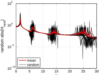
Figure 7 shows some Monte Carlo simulations of the response atζ= 0.3 for δ=0.2 together with the mean of the stochastic simulation. Although each random response presents well defined peaks, the mean does not have the same pattern. Figure 8 shows the 90% confidence envelope (yellow region) and the deterministic response of the reference model foru=1 (dashed line). A zoom image of the same (Fig. 8(b)) shows how the envelope includes the response close to the first natural frequency. There are some peaks that are not inside the 90% confidence region, which is expected. To guarantee that all peaks are inside the confidence envelope, too many Monte Carlo simulations would be necessary and the confidence region would have to be constructed for a value close to one, instead of 90% (see Fig. 9 for a comparison of different confidence regions). Another thing that should be remarked is that even though it seems that the stochastic response is damped because of the statistical envelopes shown in Fig. 8, each random response happens to have small damping, as shown in Fig. 7.
0 5 10 15 20 25 30
10−10 10−5 100 105
ω
random abs(H
rand
)
mean random
Figure 7. Random response of the system atζ=0.3forδ=0.2: Monte Carlo simulations and mean response of the stochastic system.
Figure 10 shows the same graphic of Fig. 8 forδ=0.5 andu=2. At this point the confidence envelope is already too large, given results that might be of no relevance.
It should be noticed that the value of δ used in the analysis depends on the dimensionless fluid velocityu, and also on the strategy employed for the calibration procedure. For instance, other natural frequencies could be used to calibrate the dispersion parameterδ, leading to different values. If the fourth natural frequency was used in the calibration procedure, the statistical envelope would be tighter in the region of the fourth natural frequency; however, the consequence would be that the first natural frequency would not be included in the statistical envelope.
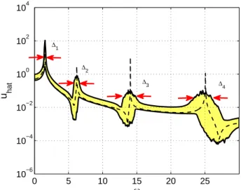
As a practical application for these results, an information that is used in the design of a structure are the values of its natural frequencies; there should not be an exciting force with frequency close to the natural frequency of the structure. In this sense, how can the stochastic model be used? Figure 11 shows the spread of the statistical envelope near the natural frequencies. Note that all∆’s increase with the natural frequency (0.3 Hz (for the 1st nat freq), 1.0 Hz (for the 2nd nat freq), 2.0 Hz (for the 3rd nat freq), 3.0 Hz (for
ω |u hat
|
0 5 10 15 20 25
10−4 10−2 100 102
(a)
ω |u hat
|
0.5 1 1.5 2 2.5
100 101 102
(b) Figure 8. Random response of the system atζ=0.3forδ=0.2. The filled region corresponds to the 90% confidence envelope and the dashed line corresponds to the deterministic response foru=1. (a) absolute value and (b) zoom close to the first natural frequency.
0 5 10 15 20 25 30
10−6 10−4 10−2 100 102 104
reference 90% 95% 99%
Figure 9. Random response of the system atζ=0.3forδ=0.2for different confidence regions (90%, 95% and 99%); the dashed line corresponds to the deterministic response foru=1.
ω |u hat
|
0 5 10 15 20 25
10−4 10−2 100 102
(a)
ω |u hat
|
0.5 1 1.5 2 2.5 3 100
101
(b) Figure 10. Random response of the system atζ=0.3forδ=0.5. The filled region corresponds to the 90% confidence envelope and the dashed line corresponds to the deterministic response foru=2. (a) absolute value and (b) zoom close to the first natural frequency.
is [10,15]Hz, the band [13,15]Hz (near the third natural frequency) should be avoided, which is a worse scenario. If one is interested in the low frequencies, anduis not big (which means thatδis also not big), then the stochastic model (incomplete model together with the nonparametric approach) is robust (thin confidence region) and the stochastic model could be used as a prediction tool. If one is interested in the medium to high frequencies, then the stochastic model is not robust (wide confidence limit), and its use is not recommended.
Concluding Remarks
This paper has analyzed the dynamics of a structure excited by internal flow, where there are model uncertainties related to the stiffness of the system due to unmodeled phenomena (the fluid stiffness). This unmodeled phenomenon was chosen arbitrarily, such that model uncertainties could be analyzed. Uncertainties within the model (modeling errors or model form uncertainty) are very challenging to take into account; and it is still a fruitful domain of research.
In the present work, these uncertainties have been modeled with the nonparametric probabilistic approach, and the stochastic system has been investigated using a simple, but non-trivial example. First, a procedure has been proposed to calibrate the dispersion parameter related to the stochastic model. Next, the spectrum of the response has been analyzed, showing how the confidence envelope changes for
ω
u hat
0 5 10 15 20 25
10−6 10−4 10−2 100 102 104
∆2
∆4 ∆3
∆1
Figure 11. Random response of the system atζ=0.3forδ=0.2. The filled region corresponds to the 90% confidence envelope and the dashed line corresponds to the deterministic response foru=1. The arrows show how wide is the statistical envelope near the natural frequencies.
different values of the dispersion parameter.
If one thinks of the solutions of the incomplete and the reference problem as points in an abstract metric space they are a certain distance apart from each other, since they are different. The strategy of the nonparametric probabilistic approach is to make a discretization of the operators random. With this, one generates a variety of solutions for the incomplete model, one for every realization. The idea is to find a sequence of realizations of the incomplete model whose solutions converge to the solution of the reference model, hence reducing the distance among the variety of solutions of the incomplete and the reference model. Now, the distance of the set of solutions of the incomplete model and the solution of the reference model is zero.
Of course, there is no perfect model. Some aspects of the real structure are not modeled and this strategy seems to give a way to approximate the reference model even if one does not know the unmodeled aspects. One drawback is that one randomizes one of the approximations of the operator, a matrix, and not the operator itself. But today, to randomize directly the operator is an unsolved problem since it is hard to define a probability space in infinite dimensions; one can do this only in special cases.
It can be concluded that by using the incomplete computational model together with the nonparametric probabilistic approach, it is possible to include the results of the reference model. As the model uncertainty depends on the dimensionless flow velocityu, ifu=0 the incomplete model gives the same results of the reference model (with
δ=0). Asuincreases, the dispersion parameterδhas to increase to encompass the response of the reference model. At certain values of uandδ, the statistical envelope gets so wide that the results might not be satisfactory. But, for smallu’s andδ’s, the incomplete model together with the nonparametric probabilistic approach have shown good results (if one is interested in the low frequencies).
the stochastic model.
Acknowledgements
The authors gratefully acknowledge the support of the Brazilian agencies CNPq, CAPES and FAPERJ.
References
Ayyub, B.M., Klir, G.J., 2006, “Uncertainty Modeling and Analysis in Engineering and the Sciences”, Chapman and Hall/CRC, USA.
Beck, J.L., Katafygiotis, L.S., 1998, “Updating models and their uncertainties: Bayesian statistical framework”, Journal of Engineering Mechanics, 124 (4), pp. 455-461.
Ben-Haim, Y., 2006, “Info-Gap Decision Theory”, Second Edition: Decisions Under Severe Uncertainty, 2nd Edition. Academic Press.
Caers, J., 2011, “Modeling Uncertainty in the Earth Sciences”, Wiley, USA.
Curling, L.R., Paidoussis, M.P., 2003, “Analyses for random flowinduced vibration of cylindrical structures subjected to turbulent axial flow”,Journal of Sound and Vibration, 264, pp. 795-833.
Jaynes, E., 2003, “Probability Theory: The Logic of Science”. Vol. 1. Cambridge University Press, Cambridge, UK.
Mehta, M.L., 1991, “Random Matrices”, 2nd Edition. Academic Press, San Diego, CA.
Paidoussis, M.P., 1998, “Fluid-Structure Interactions: Slender structures and Axial Flow”, Vol. 1, Academic Press, London, United Kingdom.
Rinaldi, S., Prabhakar, S., Vengallatore, S., Paidoussis, M.P., 2010, “Dynamics of microscale pipes containing internal fluid flow”,Journal of Sound and Vibration, 329, pp. 1081-1088.
Ritto, T.G., Sampaio, R., Cataldo, E., 2008, “Timoshenko beam with uncertainty on the boundary conditions”, Journal of the Brazilian Society ofMechanical Sciences and Engineering, 30 (4), pp. 295-303.
Ritto, T.G., Soize, C., Sampaio, R., 2009, “Nonlinear dynamics of a drill-string with uncertain model of the bit-rock interaction”.International Journal of Non-Linear Mechanics, 44 (8), pp. 865-876.
Roy, C.J., Oberkampf, W.L., 2011, “A comprehensive framework for verification, validation, and uncertainty quantification in scientific computing”,Computer Methods in Applied Mechanics and Engineering, 200 (25).
Sampaio, R., Cataldo, E., 2010, “Comparing two strategies to model uncertainties in structural dynamics”,Shock and Vibration, 17 (2), 171-186.