ISSN 0101-8205 www.scielo.br/cam
Generalizations of Aitken’s process for accelerating
the convergence of sequences
CLAUDE BREZINSKI1 and MICHELA REDIVO ZAGLIA2
1Laboratoire Paul Painlevé, UMR CNRS 8524, UFR de Mathématiques Pures et Appliquées, Université des Sciences et Technologies de Lille, 59655 – Villeneuve d’Ascq cedex, France
2Università degli Studi di Padova, Dipartimento di Matematica Pura ed Applicata Via Trieste 63, 35121 – Padova, Italy
E-mails: Claude.Brezinski@univ-lille1.fr / Michela.RedivoZaglia@unipd.it
Abstract. When a sequence or an iterative process is slowly converging, a convergence accel-eration process has to be used. It consists in transforming the slowly converging sequence into a new one which, under some assumptions, converges faster to the same limit. In this paper, new scalar sequence transformations having a kernel (the set of sequences transformed into a constant sequence) generalizing the kernel of the Aitken’s12process are constructed. Then, these trans-formations are extended to vector sequences. They also lead to new fixed point methods which are studied.
Mathematical subject classification: Primary: 65B05, 65B99; Secondary: 65H10. Key words:convergence acceleration, Aitken process, extrapolation, fixed point methods.
1 Introduction
When a sequence(Sn)of real or complex numbers is slowly converging, it can be transformed into a new sequence(Tn)by asequence transformation. Aitken’s
12process and Richardson extrapolation (which gives rise to Romberg’s method for accelerating the convergence of the trapezoidal rule) are the most well known sequence transformations. It has been proved that a sequence transformation able to accelerate the convergence of all sequences cannot exist [8] (see also [7]).
In fact, each transformation is only able to accelerate the convergence of special classes of sequences. This is the reason why several sequence transformations have to be constructed and studied.
For constructing a new sequence transformation, an important object is its kernel(we will explain why below). It is the set of sequences(Sn), characterized by a particular expression or satisfying a particular relation between its terms, both involving an unknown parameterS(the limit of the sequence if it converges or its antilimit if it does not converge), that are transformed into the constant sequence(Tn= S). For example, the kernel of the Aitken’s12process (see its definition below) is the set of sequences of the formSn=S+aλn,n=0,1, . . ., wherea 6= 0 andλ 6= 1 or, equivalently, satisfying the relation a0(Sn −S)+ a1(Sn+1−S), forn = 0,1, . . ., witha0a1 6= 0 anda0+a1 6= 0. If|λ| < 1, then(Sn) converges to its limit S. Otherwise, S is called the antilimit of the sequence(Sn).
The construction of a sequence transformation having a specific kernel consists in giving the exact expression of the parameter S for any sequence belonging to this kernel. This expression makes use of several consecutive terms of the sequence starting from Sn, and it is valid for all n. Thus, by construction, for alln, Tn = S. When applied to a sequence not belonging to its kernel, the transformation produces a sequence(Tn) which, under some assumptions, converges toSfaster than(Sn), that is
lim n→∞
Tn−S Sn−S
=0.
In that case, it is said that the transformation accelerates the convergence of(Sn).
of its kernel satisfy(Sn−S)/λn = a. Applying the usual forward difference operator1(it is an annihilation operator as will be explained below) to both sides leads to1((Sn−S)/λn) =1a =0. Thus Sn+1−S =λ(Sn−S)and it followsS =(Sn+1−λSn)/(1−λ). The problem is now to computeλ. Apply-ing the operator1to Sn = S +aλn gives1Sn = aλn(λ−1), and we obtain
λ = 1Sn+1/1Sn. Thus, replacingλ by this expression in the formula for S, leads to the transformation
Tn =
SnSn+2−Sn2+1 Sn+2−2Sn+1+Sn
, n=0,1, . . . (1)
which, by construction, has a kernel including all sequences of the form Sn = S+aλnor, equivalently, such thatSn+1−S=λ(Sn−S)for alln. We see that the denominator in this formula is12S
n, thus the name of the transformation. An important point to notice for numerical applications is that Formula (1) is numerically unstable. It has to be put under one of the equivalent forms
Tn = Sn−
(1Sn)2 Sn+2−2Sn+1+Sn = Sn+1−
1Sn1Sn+1 Sn+2−2Sn+1+Sn
= Sn+2−
(1Sn+1)2 Sn+2−2Sn+1+Sn
which are more stable. Indeed, when the termsSn,Sn+1andSn+2are close toS, a cancellation appears in Formula (1). Its numerator and its denominator are close to zero, thus producing a first order cancellation. A cancellation also appears in the three preceding formulae, but it is a cancellation on a correcting term, that is, in some sense, a second order cancellation (see [5, pp. 400–403] for an extensive the discussion).
By construction, we saw that, for alln,Tn = S, if(Sn)belongs to the kernel of the transformation. To prove that this condition is also necessary is more difficult. One has to start from the condition for alln,Tn =S, and then to show that it implies that the relation defining the kernel is satisfied. This is why, in this paper, we will only say that the kernels of the transformations studied include all sequences having the corresponding form since additional sequences can also belong to the kernel. Let us mention that, for the Aitken’s process, the condition is necessary and sufficient.
Of course, one can ask why the notion of kernel is an important one. Although this result was never proved, it is hoped (and it was experimentally verified) that if a sequence is not “too far away” from the kernel of a certain transformation, then this transformation will accelerate its convergence. For example, the kernel of the Aitken’s process can also be described as the set of sequences such that for alln, (Sn+1−S)/(Sn−S) = λ 6= 1. It is easy to prove that this process accelerates the convergence of all sequences for which there existsλ6= 1 such that limn→∞(Sn+1− S)/(Sn −S) = λ. On sequence transformations, their kernels, and extrapolation methods see, for example, [5, 14, 16].
(that is a kind of second order term) to the sequence as pointed out by Weniger [15]. Let us mention that, as showed in particular in [13], there is a strong connection between asymptotics and extrapolation methods.
In Section 5, these transformations will be extended to vector sequences. The related fixed point methods will be studied in Section 6.
The following definitions are needed in the sequel. The forward difference operator1is defined by
1un = un+1−un,
1k+1un = 1kun+1−1kun, the divided difference operatorδis defined by
δun =
un+1−un xn+1−xn
,
δk+1un =
δkun+1−δkun xn+k+1−xn and the reciprocal difference operators by
̺k+1un = ̺k−1un+1+
xn+k+1−xn
̺ku
n+1−̺kun with̺−1u
n =0 and̺0un =un.
We also remind the Leibniz’s rule for the operator1
1(unvn)=un+11vn+vn1un.
2 A first scalar kernel
We will construct a sequence transformation with a kernel containing all se-quences of the form
Sn =S+(a+bxn)λn, n =0,1, . . . (2)
whereS,a,bandλare unknown (possibly complex) numbers and(xn)a known (possibly complex) sequence.
We have, for alln,
δ(a+bxn)=δ
Sn−S
λn
2.1 First technique
From (3), we obtain
bλn+11xn =Sn+1−S−λ(Sn−S). (4) Extracting Sfrom this relation leads to a first transformation whose kernel in-cludes all sequences of the form (2)
Tn=
Sn+1−λSn−bλn+11xn
1−λ , n=0,1, . . . (5)
The problem is now to compute the unknowns b and λ (or λ and bλn+1) appearing in (5). Applying the forward difference operator1to (4), we get
bλn+1(λ1xn+1−1xn)=1Sn+1−λ1Sn, (6) which givesb(orbλn+1) ifλis known.
Writing down (6) also for the indexn+1, we obtain a system of two nonlinear equations in our unknowns. The unknown productbλn+1can be eliminated by division and we get, after rearrangement of the terms,
1Sn+2−λ1Sn+1
λ1xn+2−1xn+1
=λ1Sn+1−λ1Sn λ1xn+1−1xn
. (7)
This is a cubic equation which provides, in the real case, a uniqueλonly if it has one single real zero. So, another procedure for the computation ofλhas to be given.
It is possible to computeλ by writing this cubic equation for the indexesn, n+1 andn+2. Thus we obtain a system of 3 linear equations in the 3 unknowns
λ, λ2, andλ3
αn+iλ3+βn+iλ2+γn+iλ=δn+i, i =0,1,2 with
αn+i = 1xn+2+i1Sn+i
βn+i = −(1xn+1+i1Sn+1+i +1xn+2+i1Sn+1+i+1xn+1+i1Sn+i)
γn+i = 1xn+1+i1Sn+2+i +1xn+i1Sn+1+i +1xn+1+i1Sn+1+i
We solve this system for the unknownλ, then we computeλn+1, and we finally obtainbby (6).
Another way to proceed is to replacebλn+1by its expression in (5). Then the transformation can also be written as
Tn =
λrn(Sn+1−λSn)−(Sn+2−λSn+1)
(λrn−1) (1−λ)
, (8)
= Sn+1−
1Sn+1−λ2rn1Sn
(λrn−1)(1−λ)
, (9)
withrn =1xn+1/1xn, and whereλis computed by solving the preceding linear system. Formula (9) is more stable than Formula (8). In (9), it is also possible to replaceλ2 by its value given as the solution of the preceding linear system instead of squaringλ, thus leading to a different transformation with also a kernel containing all sequences of the form (2).
Remark 1. Obviously, for sequences which do not have the form (2), the value ofλobtained by the previous procedures depends onn.
If 1xn is constant, λ = 1 satisfies the preceding system but its matrix is singular. In this case, (7) reduces to
1Sn+2−λ1Sn+1=λ(1Sn+1−λ1Sn) andλcan be computed by solving the system
1Sn+iλ2−21Sn+1+iλ= −1Sn+i+2, i=0,1. Then, the transformation given by (8) or (9) becomes
Tn =
(Sn+2−λSn+1)−λ(Sn+1−λSn)
(λ−1)2 , (10)
= Sn+1+
1Sn+1−λ21Sn
(λ−1)2 . (11)
Formula (11) is more stable than (10).
Let us give a numerical example to illustrate this transformation. We consider the sequence
with xn = nα. We took S = 1, λ = 1.15, α = 3.5, and b = 2. With these values, the first term in(Sn)diverges, while the second one tends to zero and, according to [15], is a subdominant contribution to (Sn). On Figure 1, the solid lines represent, in a logarithmic scale, and from top to bottom, the absolute errors of Sn, of the Aitken’s 12 process (which uses 3 consecutive terms of the sequence to accelerate), of its first iterate (which uses 5 terms), and of its second iterate (which uses 7 terms). The dash-dotted line corresponds to the error of (11) (which uses 5 terms) with xn defined as above (which im-plies the knowledge ofα), and the dashed line to the error of (9) (which uses 6 terms). Iterating a process, such as Aitken’s, consists in reapplying it to the new sequence obtained by its previous application. On this example, the numerical results obtained by the Formula (8) and by the more stable Formula (9) are the same. The computations were performed using Matlab 7.3.
0 10 20 30 40 50
−4 −2 0 2 4 6 8 10
Figure 1 – Transformation (9) in dashed line, and transformation (11) in dash-dotted line, both applied to (12).
and (11), and they generate sequences which converge before diverging again. Of course, whenngrows, the subdominant contribution is almost zero, and this is why these sequence transformations no longer operate. This is particularly visible with transformation (11) which produces a rapidly diverging sequence. On the contrary, transformation (9) exhibits a behavior similar to the behavior of an asymptotic series. Thus stopping its application after 27 or 28 terms leads to an error of the order of 10−4. It must be noticed that the numerical results are quite sensitive to changes in the parametersα,λ, andbif Formula (10) is used, while they are not with Formula (11).
2.2 Second technique
Since, for alln,δ(a+bxn)is a constant, then for alln,1δ(a+bxn)=0. Thus
0 = 1δ
Sn−S
λn
= 1
λn+2
Sn+2−S−λ(Sn+1−S)
1xn+1
−λSn+1−S−λ(Sn−S) 1xn
and it follows, forn=0,1, . . .,
1xn[Sn+2−S−λ(Sn+1−S)] −λ1xn+1[Sn+1−S−λ(Sn−S)] =0. (13) ExtractingSfrom this relation, we obtain the following sequence transforma-tion whose kernel includes all sequences of the form (2)
Tn =
Sn+21xn−λSn+1(1xn+1xn+1)+λ2Sn1xn+1
1xn−λ(1xn+1xn+1)+λ21xn+1
(14)
= Sn+1+
1Sn+11xn−λ21Sn1xn+1
1xn−λ(1xn+1xn+1)+λ21xn+1
. (15)
Formula (15) is more stable than (14).
to (13), we get, for alln,
L(Sn+21xn)−λL(Sn+1(1xn+1xn+1))+λ2L(Sn1xn+1)=0. (16) This polynomial equation of degree 2 has 2 solutions and we don’t know which solution is the right one. So, we will compute simultaneouslyλandλ2. For that, we write (16) for the indexesnandn+1, and we obtain a system of two linear equations in these two unknowns
λL(Sn+1(1xn+1xn+1))−λ2L(Sn1xn+1) = L(Sn+21xn)
λL(Sn+2(1xn+1+1xn+2))−λ2L(Sn+11xn+2) = L(Sn+31xn+1). It must be noticed that this approach requires more terms of the sequence than solving directly the quadratic equation (16) forλ.
The solution of the system is
λ = L(Sn+31xn+1)L(Sn1xn+1)−L(Sn+21xn)L(Sn+11xn+2)
/Dn
λ2 = L(Sn+31xn+1)L(Sn+1(1xn+1xn+1))
−L(Sn+21xn)L(Sn+2(1xn+1+1xn+2))
/Dn
with
Dn = L(Sn1xn+1)L(Sn+2(1xn+1+1xn+2))
−L(Sn+11xn+2)L(Sn+1(1xn+1xn+1)).
Replacing λ and λ2 in (14) or (15) completely defines our sequence trans-formation. Let us remark that, for sequences which are not of the form (2), a different transformation is obtained if the preceding expression forλis used in (14) or (15), and then squared for gettingλ2.
Remark 2. The annihilation operator L used for obtaining (16) from (13)
must be independent ofn since it has to be applied to a linear combination of terms of the sequence(xn)whose coefficients can depend onn. SoLcannot be
Let us mention that annihilation operators are only known for quite simple sequences. For example, the annihilation operator corresponding toxn = nk is L ≡ 1k+1, since 1k+1nk = 1k(1nk). If, for all n, x
n is constant, the transformation (11) is recovered.
This construction could be extended to a kernel whose members have the formSn = S+Pk(xn)λn, where Pk is a polynomial of degreek. Indeed, since
δkPk(xn)is a constant, we have, for alln,
1δkPk(xn)=1δk
Sn−S
λn
=0.
However, the difficulty in applying the two techniques described above lies in the derivation and the solution of a system of equations involvingλand its powers. We will not pursue in this direction herein.
3 A second scalar kernel
We will now construct a sequence transformation with a kernel containing all sequences of the form
Sn=S+
λn
a+bxn
, n=0,1, . . . (17)
whereS,a,bandλare unknown scalars and(xn)a known sequence. We have, for alln,δ(a+bxn)=δ(λn/(Sn−S))=b. Thus
λn
λ
Sn+1−S
− 1
Sn−S
=b1xn,
which is a nonlinear equation in S. Therefore the problem is to bypass such a nonlinearity.
We have, for alln,
1δ(a+bxn)=1δ
λn
Sn−S
=0,
and, therefore,
λ1xn
λ
Sn+2−S
− 1
Sn+1−S
−1xn+1
λ
Sn+1−S
− 1
Sn−S
=0.
Settingen =Sn−Sand reducing to the same denominator, we have
3.1 First technique
The main drawback of (18) is that it is a quadratic equation in S. Let us con-sider the particular case where1xn is constant. If we apply the operator 1, then, by Leibniz’s rule, 1(en+pen+q) = en+p+11en+q + en+q1en+p. Since
1en+i = 1Sn+i, we obtain a linear expression in S. Remark that, for each product en+pen+q, we can choose, in Leibniz’s rule, either un = en+p and
vn=en+qor vice versa. However, after simplification, all these choices lead to the same expression.
Applying1to (18), we obtain, when1xnis constant,
λ2(en+21Sn+en1Sn+1)−2λ(en+11Sn+2+en+21Sn) +(en+31Sn+1+en+11Sn+2)=0.
(19)
Define the transformation
Tn = Nn Dn
(20)
with
Nn = λ2Sn+1(Sn+2−Sn)−2λ(Sn+3Sn+1−Sn+2Sn)+Sn+2(Sn+3−Sn+1) Dn = λ2(Sn+2−Sn)−2λ(Sn+3−Sn+2+Sn+1−Sn)+(Sn+3−Sn+1). Then, by (19), the kernel of the transformation (20) includes all the sequences of the form (17).
It remains to compute λ, and the problem can be solved as above. If, in (19), we do not separateλandS, the unknowns areλ2,λ,λ2S,λS andS. So, writing (19) for the indexesn, . . . ,n+4, leads to a system of 5 linear equations in these 5 unknowns
λ2Sn+1+i(Sn+2+i −Sn+i)−2λ(Sn+1+iSn+3+i −Sn+iSn+2+i) −λ2S(Sn+2+i −Sn+i)+2λS(Sn+3+i −Sn+2+i+Sn+1+i −Sn+i) −S(Sn+3+i −Sn+1+i)= −Sn+2+i(Sn+3+i −Sn+1+i), i =0, . . . ,4,
(21)
which providesλandλ2.
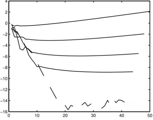
Let us give a numerical example to illustrate this transformation. We consider the sequence
Sn = S+
λn
2+αn + b n
nβ, n =0,1, . . . (22)
We took S = 1, λ = −1.2,b = 0.1, α = 1.1, and β = 2.5. With these values, the first term in(Sn)diverges, while the second one tends to zero. This second term is a subdominant contribution to(Sn). On Figure 2, the solid lines represent, in a logarithmic scale, and from top to bottom, the absolute errors of Sn, of the Aitken’s12process (which uses 3 consecutive terms of the sequence to accelerate), of its first iterate (which uses 5 terms), and of its second iterate (which uses 7 terms). The dashed line corresponds to the error of (20) (which uses 8 terms).
0 10 20 30 40 50
−16 −14 −12 −10 −8 −6 −4 −2 0 2 4
Figure 2 – The transformation (20) applied to (22), in dashed line.
3.2 Second technique
Equation (18) can be written as
λ2SnSn+11xn−λSnSn+2(1xn+1xn+1)+Sn+1Sn+21xn+1
−S[λ2(Sn+Sn+1)1xn−λ(Sn+Sn+2)(1xn+1xn+1)
+(Sn+1+Sn+2)1xn+1] = S2(λ−1)[1xn+1−λ1xn].
(23)
Remark 3. If the reciprocal difference operator is applied to the sequence
1/(a+bxn) = (Sn −S)/λn, we get, for alln, ̺2(1/(a +bxn)) = ̺2((Sn − S)/λn)=0, and (18) is exactly recovered.
For extractingSfrom (23), we need to know an annihilation operatorLfor the sequence(1xn+1−λ1xn), and we obtain the following transformation whose kernel includes all sequences of the form (17)
Tn= Nn Dn
. (24)
Here
Nn = L(λ2SnSn+11xn−λSnSn+2(1xn+1xn+1)+Sn+1Sn+21xn+1) Dn = L(λ2(Sn+Sn+1)1xn−λ(Sn+Sn+2)(1xn+1xn+1)
+ (Sn+1+Sn+2)1xn+1).
4 Other transformations
Let us now discuss some additional transformations.
In the particular casexn =n, the following transformation also has a kernel including all sequences of the form (2). It was obtained by Durbin [10], and it is defined as
Tn =
3S2
n+2−4Sn+1Sn+3+SnSn+4 6Sn+2−4(Sn+1+Sn+3)+(Sn+Sn+4)
, n =0,1, . . . (25)
Let us mention that, in this particular case, the second Shanks transformation (the fourth column of theε-algorithm)e2:(Sn)7−→ e2(Sn)=ε(4n)
also has a kernel containing all sequences of the form (2), see [4].
We remark that the denominator of (25) is14S
n, and it is easy to see that this transformation can also be written as
Tn =
Sn1Sn+3−3Sn+11Sn+2+3Sn+21Sn+1−Sn+31Sn
1Sn+3−31Sn+2+31Sn+1−1Sn
.
This expression leads to the idea of other transformations of a similar form with a denominator equal to
1k+1Sn = 1k(1Sn) = k
X
i=0
(−1)iCki1Sn+k−i,
whereCki =k!/(i!(k−i)!)is the binomial coefficient. So, we obtain a whole class of transformations defined by
Tn = k
X
i=0
(−1)iCkiSn+i1Sn+k−i
k
X
i=0
(−1)iCki1Sn+k−i
.
The kernels of these transformations are unknown, but it is easy to see that they all contain the kernel of the Aitken’s process. These transformations have to be compared with the1k processes [9] given by
Tn=
1k(Sn/1Sn)
1k(1/1S n)
= k
X
i=0
(−1)iCkiSn+k−i/1Sn+k−i
k
X
i=0
(−1)iCki/1Sn+k−i
The casek = 1 corresponds to the Aitken’s12 process and, fork = 2, the second columnθ2(n)of theθ-algorithm is recovered (see [5]). The kernel of this transformation is the set of sequences such that, for alln,
1k
Sn−S
1Sn
= 0,
that is
Sn−S
1Sn
= Pk−1(n) , wherePk−1is a polynomial of degreek−1 inn.
5 The vector case
The sequence transformations described in Sections 2 and 3 will now be used in the case whereSnandSare vectors of dimension p. Obviously, for a vector sequence, a scalar transformation could be used separately on each component. However, such a procedure is usually less efficient than using a transformation specially built for treating vector sequences.
We begin by the first kernel studied in Section 2. Different situations could be considered
Sn=S+(a+bxn)λnorSn=S+(a+xnb)λn
λ∈C a∈Cp bx
n∈Cp xnb∈Cp
b∈C,xn ∈Cp b∈Cp,xn ∈C
b∈Cp×p,x
n ∈Cp b∈Cp,xn ∈Cp×p
λ∈Cp a∈C b∈C,xn ∈C
or bxn∈Cp×p xnb∈Cp×p a∈Cp×p b∈C,x
n ∈Cp×p b∈Cp×p,xn ∈C b∈Cp×p,x
n ∈Cp×p b∈Cp×p,xn ∈Cp×p Sn=S+λn(a+bxn)orSn=S+λn(a+xnb)
λ∈Cp×p a∈Cp bxn∈Cp xnb∈Cp
b∈C,xn ∈Cp b∈Cp,x n ∈C b∈Cp×p,x
Let us consider the first transformation in the case whereλandbare scalars, anda and xn vectors. Formulae (5) and (6) are still valid. Taking the scalar product of (6) with two linearly independent vectorsy1andy2, and eliminating bgives
λ(y1, 1xn+1)(y2, 1Sn+1)−(y2, 1xn+1)(y1, 1Sn+1)
+ (y1, 1xn)(y2, 1Sn)−(y2, 1xn)(y1, 1Sn)
+ λ2(y2, 1xn+1)(y1, 1Sn)−(y1, 1xn+1)(y2, 1Sn)
= (y1, 1xn)(y2, 1Sn+1)−(y2, 1xn)(y1, 1Sn+1).
Writing down this relation also for the index n+1 leads to a system of two equations in the two unknowns λ and λ2, which completely defines the first vector transformation.
Another way of computingλandλ2consists in writing down (6) for the indexes nandn+1 and taking the scalar products with a unique vectory. Eliminating bgives an equation in our two unknowns. Then, this equation is written down for the indexesn andn+1, thus leading again to a system of two equations.
For the second transformation, nothing has to be changed until (16) included. For the computation ofλandλ2one can proceed as for the first transformation. The relation (16) can be multiplied scalarly byy1andy2. Thus, a system of two equations is obtained for the unknowns. It is also possible to write down (16) for the indexesnandn+1 and to multiply these two equations scalarly by the same vectory.
For the second kernel considered in Section 3, it can be written as Sn = S+(a+bxn)−1λn, which shows thata+bxn can be a matrix andλa vector. Obviously,aandbxncannot be vectors. This second kernel can then be treated in a way similar to the first one.
6 Fixed point methods
There is a close connection between sequence transformations and fixed point iterations for findingx ∈ Rpsuch thatx = F(x), where F is a mapping ofRp
to obtaining Steffensen’s method from Aitken’s12 process in the case p =1. The transformations obtained in this way are often related to quasi-Newton meth-ods; see [3].
In each sequence transformation, the computation of Tn makes use of Sn, . . . , Sn+m, where the value ofm differs for each of them. An iteration of a fixed point method based on a sequence transformation consists in the following steps for computing the new iteratexn+1from the previous onexn
1. SetS0=xn.
2. ComputeSi+1= F(Si)fori =0, . . . ,m−1.
3. Apply the sequence transformation toS0, . . . ,Sm, and computeT0.
4. Setxn+1=T0.
7 Conclusions
In this paper, we discussed how to construct scalar sequence transformations with certain kernels generalizing the kernel of the Aitken’s12process. As we could see, generalizations for the types of kernels we considered are not so easy to obtain and the corresponding algorithms need some efforts to be imple-mented. However, we experimented some cases where they were quite effective. The convergence and the acceleration properties of these transformations remain to be studied. Then, we showed how extend some of these transformations to the case of vector sequences. Since we only gave the idea how to proceed, a systematic study of such vector transformations and their applications have to be pursued. Finally, we explained how to convert these vector transformations into fixed point iterations. They also have to be analyzed.
REFERENCES
[1] C. Brezinski, Vector sequence transformations: methodology and applications to linear sys-tems. J. Comput. Appl. Math.,98(1998), 149–175.
[2] C. Brezinski, Dynamical systems and sequence transformations. J. Phys. A: Math. Gen.,34 (2001), 10659–10669.
[3] C. Brezinski, A classification of quasi-Newton methods. Numer. Algorithms,33(2003), 123–135.
[4] C. Brezinski and M. Crouzeix, Remarques sur la procédé12d’Aitken. C.R. Acad. Sci. Paris, 270 A(1970), 896–898.
[5] C. Brezinski and M. Redivo Zaglia,Extrapolation Methods. Theory and Practice. North-Holland, Amsterdam, 1991.
[6] C. Brezinski and M. Redivo Zaglia, Vector and matrix sequence transformations based on biorthogonality. Appl. Numer. Math.,21(1996), 353–373.
[7] J.P. Delahaye,Sequence Transformations. Springer-Verlag, Berlin, 1988.
[8] J.P. Delahaye and B. Germain-Bonne, Résultats négatifs en accélération de la convergence. Numer. Math.,35(1980), 443–457.
[9] J.E. Drummond, A formula for accelerating the convergence of a general series. Bull. Aust. Math. Soc.,6(1972), 69–74.
[10] F. Durbin, Private communication, 20 June 2003.
[11] G. Fikioris, An application of convergence acceleration methods. IEEE Trans. Antennas Propagat.,47(1999), 1758–1760.
[12] A. Navidi, Modification of Aitken’s12 formula that results in a powerful convergence accelerator, inProceedings ICNAAM-2005. T.E. Simos et al. eds., Viley-VCH, Weinheim, 2005, pp. 413–418.
[13] G. Walz,Asymptotics and Extrapolation. Akademie Verlag, Berlin, 1996.
[14] E.J. Weniger, Nonlinear sequence transformations for the acceleration of convergence and the summation of divergent series. Comput. Physics Reports,10(1989), 189–371. [15] E.J. Weniger, Private communication, 12 September 2003.