CERN-PH-EP/2013-027 2013/06/11
CMS-HIG-12-035
Search for the standard model Higgs boson produced in
association with a top-quark pair in pp collisions at the
LHC
The CMS Collaboration
∗Abstract
A search for the standard model Higgs boson produced in association with a top-quark pair is presented using data samples corresponding to an integrated
luminos-ity of 5.0 fb−1(5.1 fb−1) collected in pp collisions at the center-of-mass energy of 7 TeV
(8 TeV). Events are considered where the top-quark pair decays to either one
lep-ton+jets (tt→ `νqq0bb) or dileptons (tt→ `+ν`−νbb),`being an electron or a muon.
The search is optimized for the decay mode H → bb. The largest background to
the ttH signal is top-quark pair production with additional jets. Artificial neural net-works are used to discriminate between signal and background events. Combining the results from the 7 TeV and 8 TeV samples, the observed (expected) limit on the cross section for Higgs boson production in association with top-quark pairs for a Higgs boson mass of 125 GeV is 5.8 (5.2) times the standard model expectation.
Submitted to the Journal of High Energy Physics
c
2013 CERN for the benefit of the CMS Collaboration. CC-BY-3.0 license ∗See Appendix A for the list of collaboration members
1
Introduction
With the recent observation [1, 2] at the Large Hadron Collider (LHC) of a new, Higgs-like par-ticle with a mass of approximately 125 GeV, the focus of searches for the standard model (SM) Higgs boson has shifted to evaluating the consistency of this new particle with SM expecta-tions. A key component in this effort will be to determine whether the new particle’s observed couplings to other fundamental particles match the predictions for a SM Higgs boson. A devi-ation from expectdevi-ations could provide hints of physics beyond the standard model.
In the SM, the dominant production mechanism for the Higgs boson at the LHC arises from gluon fusion, via the Higgs boson coupling to gluons through a heavy quark loop. However, with sufficient data, other production mechanisms, such as Higgs boson production via vector boson fusion or in association with a W boson, Z boson, or tt pair, should also be observable. Furthermore, there are a number of decay channels available to a SM Higgs boson with a mass of approximately 125 GeV. Although the dominant decay mode at this mass is to a pair of bottom quarks, decays to WW, ZZ, ττ, and γγ are also experimentally accessible. The SM provides precise predictions for these production and decay rates that depend on the coupling strength of the Higgs boson to the other fundamental particles of the SM.
To date, the only combinations of production mechanism and decay mode that have been estab-lished at greater than three standard deviation (σ) significance for this newly observed particle are direct production, with the new particle decaying either to a pair of photons or a pair of W or Z bosons. In all three of these cases, the observed rates are in agreement with SM expecta-tions for Higgs boson production within the experimental uncertainties. However, establishing the complete consistency of the couplings of this newly observed particle with SM expectations for the Higgs boson involves measuring the rate of production across all the various possible production and decay channels discussed above.
The analysis described herein focuses on the search for a Higgs boson produced in association with a pair of top quarks (ttH production) conducted at the Compact Muon Solenoid (CMS) experiment. The analysis considers Higgs boson masses between 110 and 140 GeV. The search is optimized for Higgs boson decays to a bottom-quark pair, but we do not exclude events from other Higgs boson decay modes. The rate at which this process occurs depends on the largest of the fermionic couplings to the Higgs boson, namely the couplings to the top and bottom quarks. These two key couplings will be particularly important in probing the new particle’s consistency with SM expectations.
The ttH vertex is the most challenging one to probe directly. Measuring the rate of Higgs boson production through the gluon fusion process provides an indirect measurement of the coupling between the top quark and the Higgs boson because this production mechanism is dominated by a top-quark loop that couples the gluons to the Higgs boson [3]. Likewise, the decay of the Higgs boson to two photons receives a significant contribution from a top-quark loop, although the loop involving W bosons dominates in this process [4]. However, extraction of the coupling between the top quark and the Higgs boson in this way relies on the assumption that there are no new massive fundamental particles beyond those of the SM that contribute in the loop. Unless the Higgs boson is very heavy, it will not decay to top quarks. Therefore, for the mass range most favored for the SM Higgs [5], and for 125 GeV in particular, ttH production is the only way to probe the ttH vertex in a model-independent manner [6, 7].
In contrast, there are several processes that can be used to probe the coupling of this new par-ticle to bottom quarks. Because of the large bb background from multijet production, it is not
2 3 Data and simulation samples
the search is typically made using associated production involving either a W or a Z boson (VH production). Although ttH production has a smaller expected cross section, this signature pro-vides a probe that is complementary to the VH channel: they both provide information about the coupling between the bottom quark and the Higgs boson, but the dominant backgrounds
are very different, tt+jets production instead of W+jets production.
An observation of ttH production, depending on the measured properties, might be consistent with the SM Higgs boson or could indicate something more exotic [8, 9]. Since the expected SM rates in this channel are very small, a sizeable excess would be clear evidence for new physics. A previous search at the Tevatron [10], the first such search conducted at a hadron collider, showed no significant excess over SM expectation.
This paper is organized as follows. Section 2 describes the CMS apparatus. Section 3 describes the data and simulation samples utilized in the analysis, while Section 4 discusses the object identification, event reconstruction and selection. The extraction of the ttH signal is discussed in Section 5, followed by a description of the impact of systematic uncertainties encountered in the analysis in Section 6. The results of this search are reported in Section 7 and followed by a summary in Section 8.
2
The CMS detector
The CMS detector consists of the following main components. A superconducting solenoid oc-cupies the central region of the CMS detector, providing an axial magnetic field of 3.8 T parallel to the beam direction. The silicon pixel and strip tracker, the crystal electromagnetic calori-meter and the brass/scintillator hadron caloricalori-meter are located in concentric layers within the
solenoid. These layers provide coverage out to|η| = 2.5, where pseudorapidity is defined as
η =−ln[tan(θ/2)]. A quartz-fiber Cherenkov hadron forward calorimeter extends further to
|η| < 5.2. The CMS experiment uses a right-handed coordinate system, with the origin at the
nominal interaction point, the x axis pointing to the center of the LHC ring, the y axis pointing up (perpendicular to the LHC plane), and the z axis along the counterclockwise beam direction. The polar angle θ is measured from the positive z axis and the azimuthal angle φ is measured in the x-y plane in radians. Muons are detected by gas-ionization detectors embedded in the steel flux return yoke outside the solenoid. The first level of the CMS trigger system, composed of custom hardware processors, is designed to select the most interesting events in less than 3 µs using information from the calorimeters and muon detectors. The high-level trigger processor farm further decreases the event rate to a few hundred Hz for data storage. More details about the CMS detector can be found in Ref. [11].
3
Data and simulation samples
This search is performed with samples of proton-proton collisions at√s = 7 TeV and 8 TeV,
collected with the CMS detector in 2011 and 2012, respectively. These data correspond to a
total integrated luminosity of 5.0 fb−1at 7 TeV and 5.1 fb−1at 8 TeV.
All background and signal processes are modeled using Monte Carlo (MC) simulations from
MADGRAPH 5.1.1 [12], PYTHIA 6.4.24 [13], and POWHEG 1.0 [14] event generators,
depend-ing on the physics process. The MC samples use CTEQ6L1 [15] parton distribution functions
(PDFs) of the proton, except for the POWHEG samples, which use CTEQ6M. The ttH signal
events are generated using PYTHIA. The main background tt sample is generated with MAD
matched to parton showers produced by PYTHIA. The additional partons generated with the tt sample include b and c quarks in addition to light flavored quarks and gluons. Decays of τ
leptons are handled withTAUOLA2.75 [16]. MADGRAPHis also used to simulate ttW, ttZ, W +
jets, and Drell–Yan (DY) processes, with up to 4 partons in the final state. The DY contribution
includes all Z/γ∗ → `` processes with the dilepton invariant mass m`` > 10 GeV.
Single-top production is modeled with the next-to-leading order (NLO) generatorPOWHEGcombined
withPYTHIA. Electroweak diboson processes (WW, WZ, and ZZ) are simulated usingPYTHIA. All background and signal process rates are estimated using NLO or higher theoretical predic-tions. The ttH cross section [17–24] and Higgs branching fractions [25–28] used in the analysis
have NLO accuracy. The tt and diboson cross sections are calculated at NLO with MCFM[29–
31]. The single-top-quark production rates are normalized to an approximately next-to-next-to-leading order (NNLO) calculation [32–35]. The W+jets and DY+jets rates are normalized to
inclusive NNLO cross sections from FEWZ[36, 37]. The ttW and ttZ rates are normalized to
the NLO predictions from Refs. [38, 39]. These cross sections are allowed to vary within their uncertainties in the fit we use to calculate the limit.
Effects from additional pp interactions in the same bunch crossing (pileup) are modeled by
adding simulated minimum-bias events (generated withPYTHIA) to the simulated processes.
The CMS detector response is simulated using the GEANT4 software package [40]. The pileup
multiplicity distribution in MC is reweighted to reflect the luminosity profile of the observed pp collisions. We apply an additional correction factor to account for residual differences in the
jet transverse momentum (pT) spectrum due to pileup; the event-by-event correction factor is
based on the difference between simulation and data in the distribution of the scalar sum of the transverse momenta of the jets in the event. We include a systematic shape uncertainty in association with this correction factor. In addition to correcting the MC due to pileup, we also apply jet energy resolution corrections [41] and lepton and trigger efficiency scale factors to the MC events.
4
Event reconstruction and selection
This analysis selects events consistent with the production of a Higgs boson in association with a top-quark pair (see Fig. 1). In the SM, the top quark is expected to decay to a W boson and a bottom quark nearly 100% of the time. Hence different tt decay modes can be identified according to the subsequent decays of the W bosons. Here we consider two tt decay modes:
the lepton+jets mode (tt→ `νqq0bb), where one W boson decays leptonically, and the dilepton
mode (tt→ `+ν`−νbb), where both W bosons do so. For the lepton+jets case, we select events
containing an energetic, isolated, electron or muon, and at least four energetic jets, two or more of which should be identified as originating from a b quark (b-tagged) [42]. For the dilepton case, we require a pair of oppositely charged energetic leptons (two electrons, two muons, or one electron and one muon) and two or more jets, with at least two of the jets being b-tagged. Object reconstruction is based on the particle flow (PF) algorithm [43], which combines the in-formation from all CMS subdetectors to identify and reconstruct individual objects including muons, electrons, photons, and charged and neutral hadrons produced in an event. To mini-mize the impact of pileup, charged particles are required to originate from the primary vertex,
which is identified as the reconstructed vertex with the largest value of Σp2
T, where the
sum-mation includes all tracks associated with that vertex. In both channels, a significant amount of
missing transverse energy (EmissT ) should be present due to the presence of neutrinos, however
no explicit requirement on the EmissT is used in the event selection. The EmissT vector is calculated
chan-4 4 Event reconstruction and selection g g ¯t t t ¯t H W+ W− b ¯b b ¯b `+ ν` ¯ q0, ¯ν ` q, `−
Figure 1: A leading-order Feynman diagram for ttH production, illustrating the two top-quark
pair system decay channels considered here, and the H→ bb decay mode for which the
anal-ysis is optimized.
nels, we use a common set of criteria for selecting individual objects (electrons, muons, and jets) which is described below.
In the lepton+jets channel, the data were recorded with triggers requiring the presence of either a single muon or electron. The trigger muon candidate was required to be isolated from other
activity in the event and to have pT >24 GeV for both the 2011 and 2012 data-taking periods. In
2011, the trigger electron candidate was required to have transverse energy ET>25 GeV and to
be produced in association with at least three jets with pT >30 GeV, whereas in 2012, a
single-electron trigger with minimum ET threshold of 27 GeV was used. In the dilepton channel, the
data were recorded with triggers requiring any combination of electrons and muons, one lepton
with pT > 17 GeV and another with pT > 8 GeV. The offline object selection detailed below is
designed to select events in the plateau of the trigger efficiency turn-on curve.
Muons are reconstructed using information from the tracking detectors and the muon cham-bers [44]. Tight muons must satisfy additional quality criteria based on the number of hits associated with the muon candidate in the pixel, strip, and muon detectors. For lepton+jets
events, tight muons are required to have pT > 30 GeV and |η| < 2.1 to ensure the full trigger
efficiency. For dilepton events, tight muons are required to have pT > 20 GeV and|η| < 2.1.
Loose muons in both channels are required to have pT > 10 GeV and |η| < 2.4. The muon
isolation is assessed by calculating the scalar sum of the pTof charged particles from the same
primary vertex and neutral particles in a cone of ∆R =
q
(∆η)2+ (∆φ)2 = 0.4 around the
muon direction, excluding the muon itself; the resulting sum is corrected for the effects of
neu-tral hadrons from pileup interactions. The ratio of this corrected isolation sum to the muon pT
is the relative isolation of the muon. For tight muons, the relative isolation is required to be less than 0.12. For loose muons, this ratio must be less than 0.2.
Electrons are reconstructed using both calorimeter and tracking information [45]. Any elec-tron that can be paired with an oppositely charged particle consistent with the conversion of an energetic photon is rejected. Tight electrons in lepton+jets events are required to have
ET >30 GeV, while in dilepton events they must have ET >20 GeV. Loose electrons must have
ET > 10 GeV. All electrons are required to have|η| < 2.5. Electrons that fall into the transition
region between the barrel and endcap of the electromagnetic calorimeter (1.442<|η| <1.566)
are rejected because the reconstruction of an electron object in this region is not optimal. The isolation for electrons is calculated in a similar manner to muon isolation; however, for
elec-trons the isolation sum is calculated in a cone of∆R= 0.3. In the same way as for muons, the
relative isolation is the ratio of this corrected isolation sum to the electron ET. Tight electrons
must have a relative isolation less than 0.1, while loose electrons must have a relative isolation less than 0.2.
In both channels of this search, all events are required to contain at least one tight lepton, either a muon or an electron. The second lepton in the dilepton channel may be loose or tight, while in the lepton+jets channel events with a second loose lepton are rejected to ensure the same events do not enter both channels.
Jets are reconstructed by clustering the charged and neutral PF particles using the anti-kT
algo-rithm with a distance parameter of 0.5 [46, 47]. Particles identified as isolated muons and elec-trons are expected to come from W decays and are excluded from the clustering. Non-isolated muons and electrons are expected to come from b-decays and are included in the clustering. The momentum of a jet is determined from the vector sum of all particle momenta in the jet candidate and is scaled according to jet energy corrections, based on simulation, jet plus photon data events and dijet data events [41]. Charged PF particles not associated with the primary event vertex are ignored when reconstructing jets. The neutral component coming from pileup events is removed by applying a residual energy correction following the area-based proce-dure described in Refs. [48, 49]. In the lepton+jets channel, we require at least three jets with
pT > 40 GeV and a fourth jet with pT > 30 GeV. In the dilepton analysis, we require at least
two jets with pT >30 GeV. All jets must have a pseudorapidity in the range|η| <2.4.
Jets are identified as originating from a b quark using the combined secondary vertex (CSV) algorithm [42]. This algorithm combines information about the impact parameter of tracks and reconstructed secondary vertices within the jets in a multivariate algorithm designed to separate jets containing the decay products of bottom-flavored hadrons from jets originating from charm quarks, light quarks, or gluons. The CSV algorithm provides a continuous output discriminant; high values of the CSV discriminant indicate that the jet is more consistent with being a b jet, while low values indicate the jet is more likely a light-quark jet. To select b-tagged jets, a selection is placed on the CSV discriminant distribution such that the efficiency is 70% (20%) for jets originating from a b (c) quark and the probability of tagging jets originating from light quarks or gluons is 2%. In addition, the CSV discriminant values for the selected jets are used in the signal extraction as described in Section 5. For MC events, the CSV discriminant values of each jet are adjusted so that the proportion of b jets, c jets, and light-quark jets of
different η and pT values passing each of three CSV working points (tight,medium, and loose)
is the same in data and MC. The adjustment factor is computed using a linear interpolation between CSV working points.
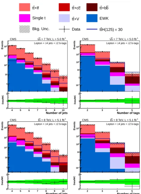
Figure 2 shows the jet and b-tagged jet multiplicities for events selected in the lepton+jets chan-nel. For both lepton+jets and dilepton channels, signal ttH events are generally characterized by having more jets and more tags than the background processes. To increase the sensitivity of this analysis, we separate the selected events into different categories based on the number of
jets and tags. For lepton+jets events, we use the following seven categories:≥6 jets + 2 b-tags,
4 jets + 3 b-tags, 5 jets + 3 b-tags,≥6 jets + 3 b-tags, 4 jets + 4 b-tags, 5 jets +≥4 b-tags, and≥6 jets
6 5 Signal extraction
≥3 b-tags. Tables 1–3 show the predicted signal, background, and observed yields in each
category for the lepton+jets and dilepton channels. Background estimates are obtained from MC after the appropriate corrections and scale factors have been applied, as described above. Given the event selection criteria and the large jet and b-tag multiplicity requirements in the lepton+jets channel, the background from QCD multijet production is negligible. Uncertain-ties in signal and background yields include both statistical and systematic sources. Sources of
systematic uncertainty are described in Section 6. In Tables 1–3, the tt+jets background is
sep-arated into the tt+bb, tt+cc, and tt+light flavor (l f ) components. The categories with higher
jet and tag multiplicities are the most sensitive to signal. We include less sensitive categories in order to better constrain the background.
The choice of event selection categories outlined above is optimized for the H → bb decay
mode. However, in the higher end of our search range—including mH = 125 GeV—other
decay modes, especially WW and ττ, can have significant standard model branching fractions. For the purposes of this search, we define any ttH event as signal, regardless of the Higgs boson decay. For most of the event selection categories defined above, the contribution from
the decay modes other than H → bb is less than 10%. The largest contribution from the
non-bb decay modes arises in the≥6 jets + 2 b-tags lepton+jets category where almost 50% of the
events come from decay modes other than H → bb. In that category H → WW dominates
the non-bb contribution. With the current optimization, the impact of the non-bb decay modes
to the analysis sensitivity is negligible as the contribution from H → bb in the most sensitive
categories is>95%.
5
Signal extraction
Artificial neural networks (ANNs) [50] are used in all categories of the analysis to further dis-criminate signal from background and improve signal sensitivity. Separate ANNs are trained for each jet-tag category, and the choice of input variables is optimized for each as well. The ANN input variables considered are related to object kinematics, event shape, and the discrim-inant output from the b-tagging algorithm. A total of 24 input variables has been considered and are listed in column 1 of Table 4. The inputs are selected from a ranked list based on ini-tial separation between signal and background. The separation of the individual variables is
evaluated using a separation benchmarkhS2i[51] defined as follows:
hS2i = 1 2 Z (ˆy S(y)− ˆyB(y))2 ˆyS(y) + ˆyB(y) dy, (1)
where y is the input variable, and ˆyS and ˆyB are the signal and background probability
den-sity functions for that input variable in the signal and background samples, respectively. The maximum number of input variables considered is determined by the statistics in the simu-lated samples used for ANN training. The number of variables per category is determined by reducing the number of variables until the minimum number of variables needed to maintain roughly the same ANN performance is reached. In the lepton+jets categories, the use of ap-proximately 10 input variables yields stable performance; using fewer inputs exhibits degraded discrimination power, and using more inputs exhibits little improvement in performance in most categories. A similar exercise was done for the dilepton categories. The choice of input variables for each jet-tag category used in the 8 TeV analysis is summarized in Table 4; the input variables for each category in the 7 TeV analysis are very similar. The input variables used in the ANN can be broken down into several classes, as detailed below.
hist_0 Entries 0 Mean 0 RMS 0 0 1 2 3 4 5 6 7 8 9 10 0 0.2 0.4 0.6 0.8 1 hist_0 Entries 0 Mean 0 RMS 0 +lf t t tt+cc tt+bb Single t tt+V EWK Bkg. Unc. Data ttH(125) × 30 Number of Jets 4 5 6 7 8 9 10 Events 1 10 2 10 3 10 4 10 -1 = 7 TeV, L = 5.0 fb s CMS 2 b-tags ≥ 4 jets + ≥ Lepton + Number of jets 4 5 6 7 8 9 10 Data/MC 0 1 2 2 3 4 Number of Tags5 Events -1 10 1 10 2 10 3 10 4 10 -1 = 7 TeV, L = 5.0 fb s CMS 2 b-tags ≥ 4 jets + ≥ Lepton + Number of tags 2 3 4 5 Data/MC 0 1 2 4 5 6 7 8 9 10 Events 1 10 2 10 3 10 4 10 2 b-tags ≥ 4 jets + ≥ Lepton + -1 = 8 TeV, L = 5.1 fb s CMS Number of jets 4 5 6 7 8 9 10 Data/MC 0 1 2 1.5 2 2.5 3 3.5 4 4.5 5 5.5 Events -1 10 1 10 2 10 3 10 4 10 2 b-tags ≥ 4 jets + ≥ Lepton + -1 = 8 TeV, L = 5.1 fb s CMS Number of tags 2 3 4 5 Data/MC 0 1 2
Figure 2: Number of jets (left) and number of b-tagged jets (right) in data and simulation for
events with≥4 jets +≥2 b-tags in the lepton+jets channel at 7 TeV (top) and 8 TeV (bottom). The
background is normalized to the SM expectation; the uncertainty band (shown as a hatched band in the stack plot and a green band in the ratio plot) includes statistical and systematic uncertainties that affect both the rate and shape of the background distributions. The ttH signal
8 5 Signal extraction
Table 1: Expected event yields for backgrounds (bkg), signal, and number of observed events in the lepton+jets channel in 7 TeV data.
≥6 jets 4 jets 5 jets ≥6 jets 4 jets 5 jets ≥6 jets 2 b-tags 3 b-tags 3 b-tags 3 b-tags 4 b-tags ≥4 b-tags ≥4 b-tags ttH(125) 6.1±0.9 2.7±1.1 4.0±1.6 3.8±1.6 0.4±0.2 1.1±0.4 1.4±0.6 tt+lf 2040±520 940±170 590±120 346±92 15.7±3.3 22.8±5.3 26.1±7.7 tt+bb 31±17 26±13 28±15 24±13 2.1±1.1 5.7±3.1 8.4±4.8 tt+cc 37.5±9.5 10.1±1.9 12.8±2.7 11.8±3.2 0.5±0.1 1.0±0.3 1.5±0.5 tt V 18.4±3.5 3.2±0.6 4.3±0.8 4.5±0.9 0.2±0.0 0.5±0.1 0.7±0.2 Single t 54.8±7.0 40.0±5.1 21.8±3.3 9.6±1.6 1.2±0.4 1.0±0.3 0.8±0.3 V+jets 41±26 21±11 4.9±4.8 0.5±0.6 0.0±0.0 0.0±0.0 0.1±0.1 Diboson 0.6±0.2 0.7±0.2 0.7±0.2 0.3±0.2 0.0±0.0 0.0±0.0 0.0±0.0 Total bkg 2230±540 1040±180 660±130 396±99 19.7±4.1 30.9±7.3 38±11 Data 2137 1214 736 413 18 37 49
Table 2: Expected event yields for backgrounds (bkg), signal, and number of observed events in the lepton+jets channel in 8 TeV data.
≥6 jets 4 jets 5 jets ≥6 jets 4 jets 5 jets ≥6 jets 2 b-tags 3 b-tags 3 b-tags 3 b-tags 4 b-tags ≥4 b-tags ≥4 b-tags ttH(125) 11.7±1.9 3.9±1.8 6.1±2.8 6.9±3.1 0.6±0.3 1.5±0.7 2.5±1.2 tt+lf 3460±940 1320±280 870±210 570±170 18.0±5.1 27.6±8.6 41±15 tt+bb 61±34 35±19 43±24 35±20 2.5±1.7 8.4±5.3 15.4±9.4 tt+cc 62±17 19.6±5.1 25.0±6.9 25.9±7.7 0.6±0.4 0.8±0.9 3.7±1.8 tt V 35.7±7.5 4.5±1.1 6.1±1.4 8.6±2.1 0.1±0.1 0.7±0.2 1.5±0.4 Single t 79±18 56±11 25.6±6.2 10.3±2.9 0.3±0.6 3.1±2.2 1.0±0.6 V+jets 53±40 5.9±6.0 0.8±0.9 0.0±0.0 0.0±0.0 0.0±0.0 0.0±0.0 Diboson 1.2±0.4 1.8±0.6 0.5±0.2 0.2±0.1 0.0±0.0 0.0±0.0 0.0±0.0 Total bkg 3760±980 1440±300 970±230 650±190 21.5±6.1 41±12 63±21 Data 3503 1646 1116 686 28 56 74
Table 3: Expected event yields for backgrounds (bkg), signal, and number of observed events in the dilepton channel in 7 TeV and 8 TeV data.
7 TeV Data 8 TeV Data
2 jets + 2 b-tags ≥3 jets +≥3 b-tags 2 jets + 2 b-tags ≥3 jets +≥3 b-tags ttH(125) 0.5±0.2 2.1±0.9 0.7±0.3 3.3±1.5 tt+lf 3280±590 109±25 4100±780 135±34 tt+bb 6.5±3.4 16.1±8.6 7.6±4.2 25±14 tt+cc 5.1±1.0 7.5±1.8 10.1±2.8 14.1±4.1 tt V 2.6±0.5 2.3±0.5 3.5±0.8 3.8±0.9 Single t 99±11 3.9±0.8 129±18 6.2±2.4 V+jets 810±190 23.5±9.7 830±200 29±13 Diboson 25.8±2.7 0.6±0.1 29.2±3.7 0.7±0.2 Total bkg 4230±660 163±35 5110±860 215±48 Data 4303 185 5406 251
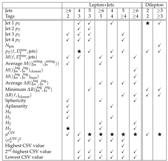
Table 4: The ANN inputs for the nine jet-tag categories in the 8 TeV ttH analysis in the lep-ton+jets and dilepton channels. The choice of inputs is optimized for each category. Definitions of the variables are given in the text. The best input variable for each jet-tag category is denoted
byF. Lepton+Jets Dilepton Jets ≥6 4 5 ≥6 4 5 ≥6 2 ≥3 Tags 2 3 3 3 4 ≥4 ≥4 2 ≥3 Jet 1 pT X X X F X Jet 2 pT X X Jet 3 pT X X X X Jet 4 pT X X X X Njets X pT(`, ETmiss, jets) F X X X X X M(`, EmissT , jets) X X X X X
Average M((juntagm , juntagn )) X X
M((jtagm , jtagn )closest) X
M((jtagm , jtagn )best) X
Average∆R(jtagm , jtagn ) X X X X
Minimum∆R(jtagm , jtagn ) X X X
∆R(`, jclosest) X X X X Sphericity X X X Aplanarity X X H0 X H1 X X H2 X X H3 F X X µCSV X X F F F F F X F (σnCSV)2 X X X X X Highest CSV value X 2nd-highest CSV value X X X X X X Lowest CSV value X X X X X X
10 5 Signal extraction
The first class of variables are those that are basic kinematic properties of single objects in the
event or combinations of objects. These variables include the pTof the leading four jets, and the
pTand mass of the system defined by the vector sum of the lepton(s) momenta, the EmissT vector,
and the momenta of the jets in the event (pT(`, EmissT , jets)and M(`, ETmiss, jets), respectively), all
of which favor larger values for ttH signal than for the backgrounds. The number of jets is
used in the≥3 jets +≥3 b-tags category in the dilepton analysis since ttH signal favors larger
jet multiplicity than background.
A related class of variables involves looking at the kinematic properties of pairs of jets. The
H → bb decay produces jets that have a large invariant mass even if the jets fail the b-tag
selection. Other untagged jets in the event tend to come from hadronic W decay and initial-or final-state radiation, and tend to have a small invariant mass compared to the jets from the Higgs boson decay. For this reason, some signal discrimination is provided by examining the invariant mass of pairs of untagged jets in lepton+jets categories with six or more jets but fewer than four b-tagged jets.
Likewise, the 6-jet category with four or more tags uses two variables that rely specifically on
the H → bb hypothesis: the invariant mass of the tagged-jet pair with the smallest opening
angle (M((jtagm , jtagn )closest)), and the “best Higgs mass” (M((jtagm , jtagn )best)), the invariant mass constructed from the two tagged jets least likely to be a part of the tt system as determined by
a minimum χ2 search among all the jet, lepton, and ETmisscombinations in the event, using the
W and top masses as kinematic constraints. The M((jtagm , jtagn )closest)distribution for both signal and background has a peak near the same value; however, the distribution is wider in the case of signal, offering some discriminating power. In signal events, the “best Higgs mass” is highly correlated with the Higgs boson mass. Although the peak is broadened by events where the wrong jets are associated with the Higgs boson decay, this variable still provides some power
in discriminating signal from background. The ≥6 jets + ≥4 b-tags uses 11 variables instead
of the typical 10 because it was shown that the addition of the “best Higgs mass” variable, uniquely designed for this jet-tag category, offers a non-negligible increase in expected ANN performance.
Another class of variables exploits differences in the “shape” of events between signal and background. In general, production of an extra massive object, in addition to top quarks tends to make ttH events more spherical in shape, while the background events are more collimated or have more jet activity. Variables in this class include angular correlations, like the opening angle between the tagged jets (∆R(jtagm , jntag)) or between the lepton and closest jet (∆R(`, jclosest)),
where in the dilepton analysis the angle is calculated with respect to the lepton leading in pT.
More complex event shape variables like sphericity and aplanarity [52], as well as the Fox–
Wolfram moments H0, H1, H2, H3 [53], also exhibit differences between signal and background.
The last class of variables used in the ANN involves the CSV discriminant values of the tagged
jets. The signal events tend to have more b jets than the dominant tt+jets background. Beyond
the simple multiplicity of tagged jets we can, however, exploit the overall b-jet content of the signal in several ways. For instance, the average and squared-deviation from this average of the
CSV discriminant values for the tagged jets (µCSV,(σCSV
n )2for the n-th tagged jet) are powerful
variables. Events with genuine b jets will have higher average CSV discriminant values and the b jets themselves will have CSV values more tightly clustered around high values than those from light-flavour or charm jets which are tagged.
Using the procedure discussed above, different variables are chosen for use in each of the dif-ferent event selection categories. This is motivated by the fact that although the tt+jets back-ground is dominant throughout, the kinematics of the events can be very distinct in different
jet multiplicity bins. Similarly, the tagging discriminant of the b jets clearly is different in events
with 2, 3 or ≥4 b-tags. Finally, the overall breakdown of the tt+jets background into tt+bb,
tt+cc and tt+light-flavor is different across the jet-tag categories, implying different variables
will be more effective in some categories than others.
In nearly all event selection categories, the variables that discriminate best between signal and background directly involve b-tagging information, such as the average CSV output value for b-tagged jets. This is natural, since the largest fraction of the backgrounds in all categories involve events with fewer b jets than the ttH generally has. However, when considering
specif-ically the tt+bb, a background very similar to the signal, the b-tagging information alone is
not as powerful, and additional information from kinematic variables and angular correlations,
such as the minimum∆R between all pairs of b-tagged jets, become important. Even so, the
tt+bb background remains difficult to separate from the ttH signal.
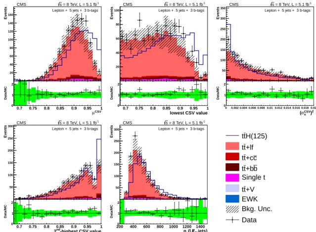
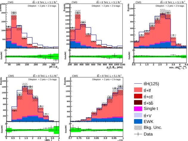
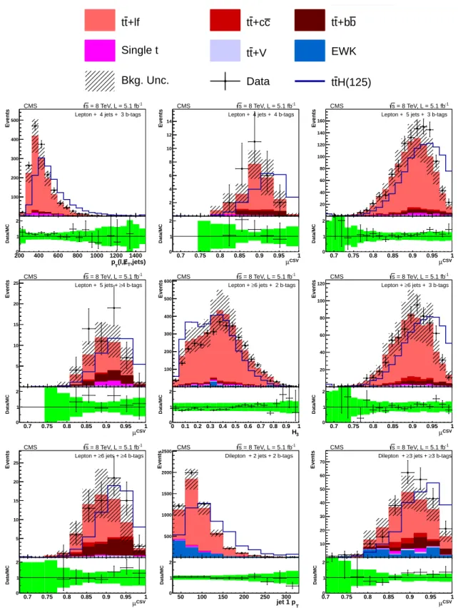
Figures 3 through 5 show the variables used in the ANN for the 5 jets + 3 b-tags category (lep-ton+jets channel) and the 2 jets + 2 b-tags (dilepton channel). The 5 jets + 3 b-tags category is chosen for lepton+jets as a compromise between signal sensitivity and adequate statistics for display purposes. Also shown, in Figure 6, are data-to-simulation comparisons of the best in-put variables for each jet-tag category considered in the 8 TeV analysis. The data-to-simulation ratio plots in Figures 3 through 6 show that, within uncertainties, the simulation reproduces well the shape and normalization of the distributions of the variables used in the ANN before the final maximum likelihood fit is performed (as discussed in Section 7). Correlations between input variables are also well reproduced by simulation.
For ANN training, we use ttH (mH = 120 GeV) as the signal and tt+jets as the background,
such that there is an equal amount of both for each category. The mass mH = 120 GeV sample
was chosen in the analysis of the 7 TeV data before the observation of a Higgs-like particle at
mH = 125 GeV was announced. This mass point was preserved in the 8 TeV ANN training for
consistency. The signal and background events used to train an ANN are split in half: one half is used to do the training itself, while the other is used as an independent test sample to monitor performance during training. The ANN method used is the “multilayer perceptron”,
available as part of theTMVA[51] package inROOT[54]. A multilayer perceptron is a specific
kind of neural network in which the neurons in each layer only have connections to neurons in the following layer. The network architecture used here consists of two hidden layers, with
N neurons in the first layer and N−1 neurons in the second layer, where N is the number of
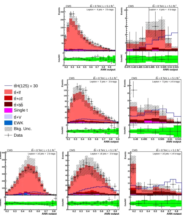
input variables. Standard tests were completed during ANN training to look for evidence of overtraining; no such evidence was found in any jet-tag category, providing confidence that our training statistics were satisfactory given the number of input variables used in each. The ANN output provides better discrimination between signal and background than any one of the input variables individually. Figures 7 and 8 show the ANN output for all the categories of the lepton+jets channel in 7 TeV and 8 TeV data, respectively, and Figs. 9 and 10 show out-put distributions for dilepton events. We use these ANN outout-put distributions for the signal extraction as described in Section 7.
6
Systematic uncertainties
Table 5 lists the systematic uncertainties that affect signal and background yields, the shape of the ANN output, or both. The effects of these uncertainties are evaluated specifically for each event selection category, and the effects from the same source are treated as completely correlated across the categories. The impact on the rate is the relative change in expected yield
12 6 Systematic uncertainties 0.7 0.75 0.8 0.85 0.9 0.95 1 Events 20 40 60 80 100 120 140 160
Lepton + 5 jets + 3 b-tags
-1 = 8 TeV, L = 5.1 fb s CMS CSV µ 0.7 0.75 0.8 0.85 0.9 0.95 1 Data/MC 0 1 2 0.7 0.75 0.8 0.85 0.9 0.95 1 Events 20 40 60 80
100 Lepton + 5 jets + 3 b-tags
-1 = 8 TeV, L = 5.1 fb s CMS lowest CSV value 0.7 0.75 0.8 0.85 0.9 0.95 1 Data/MC 0 1 2 0 0.002 0.004 0.006 0.008 0.01 0.012 0.014 0.016 0.018 0.02 Events 50 100 150 200 250 300 350
Lepton + 5 jets + 3 b-tags
-1 = 8 TeV, L = 5.1 fb s CMS 2 ) n CSV σ ( 0 0.002 0.004 0.006 0.008 0.01 0.012 0.014 0.016 0.018 0.02 Data/MC 0 1 2 0.7 0.75 0.8 0.85 0.9 0.95 1 Events 50 100 150 200 250 300
Lepton + 5 jets + 3 b-tags
-1 = 8 TeV, L = 5.1 fb s CMS -highest CSV value nd 2 0.7 0.75 0.8 0.85 0.9 0.95 1 Data/MC 0 1 2 200 400 600 800 1000 1200 1400 Events 50 100 150 200 250
300 Lepton + 5 jets + 3 b-tags
-1 = 8 TeV, L = 5.1 fb s CMS ,jets) T E (l, T p 200 400 600 800 1000 1200 1400 Data/MC 0 1 2 hist_0 Entries 0 Mean 0 RMS 0 0 1 2 3 4 5 6 7 8 9 10 0 0.2 0.4 0.6 0.8 1 hist_0 Entries 0 Mean 0 RMS 0 H(125) t t +lf t t c +c t t b +b t t Single t +V t t EWK Bkg. Unc. Data
Figure 3: Distributions of the five ANN input variables with rankings 1 through 5, in terms of separation, for the 5 jets + 3 b-tags category of the lepton+jets channel at 8 TeV. Definitions of the variables are given in the text. The background is normalized to the SM expectation; the uncertainty band (shown as a hatched band in the stack plot and a green band in the ratio plot) includes statistical and systematic uncertainties that affect both the rate and shape of
the background distributions. The ttH signal (mH = 125 GeV) is normalized to∼150× SM
0 20 40 60 80 100 120 140 160 180 200 Events 50 100 150 200 250 300
Lepton + 5 jets + 3 b-tags
-1 = 8 TeV, L = 5.1 fb s CMS T jet 3 p 0 20 40 60 80 100 120 140 160 180 200 Data/MC 0 1 2 0 50 100 150 200 250 300 Events 50 100 150 200 250
Lepton + 5 jets + 3 b-tags
-1 = 8 TeV, L = 5.1 fb s CMS T jet 2 p 0 50 100 150 200 250 300 Data/MC 0 1 2 0 50 100 150 200 250 300 350 400 Events 20 40 60 80 100 120 140 160 180 200 220
240 Lepton + 5 jets + 3 b-tags
-1 = 8 TeV, L = 5.1 fb s CMS T jet 1 p 0 50 100 150 200 250 300 350 400 Data/MC 0 1 2 0 20 40 60 80 100 120 140 160 180 200 Events 50 100 150 200 250 300 350
400 Lepton + 5 jets + 3 b-tags
-1 = 8 TeV, L = 5.1 fb s CMS T jet 4 p 0 20 40 60 80 100 120 140 160 180 200 Data/MC 0 1 2 0.5 1 1.5 2 2.5 3 3.5 4 Events 20 40 60 80 100 120 140
160 Lepton + 5 jets + 3 b-tags
-1 = 8 TeV, L = 5.1 fb s CMS ) n tag ,j m tag R(j ∆ min. 0.5 1 1.5 2 2.5 3 3.5 4 Data/MC 0 1 2 hist_0 Entries 0 Mean 0 RMS 0 0 1 2 3 4 5 6 7 8 9 10 0 0.2 0.4 0.6 0.8 1 hist_0 Entries 0 Mean 0 RMS 0 H(125) t t +lf t t c +c t t b +b t t Single t +V t t EWK Bkg. Unc. Data
Figure 4: Distributions of the five ANN input variables with rankings 6 through 10, in terms of separation, for the 5 jets + 3 b-tags category of the lepton+jets channel at 8 TeV. Definitions of the variables are given in the text. The background is normalized to the SM expectation; the uncertainty band (shown as a hatched band in the stack plot and a green band in the ratio plot) includes statistical and systematic uncertainties that affect both the rate and shape of
the background distributions. The ttH signal (mH = 125 GeV) is normalized to∼150× SM
14 6 Systematic uncertainties 50 100 150 200 250 300 Events 500 1000 1500 2000 2500 -1 = 8 TeV, L = 5.1 fb s CMS
Dilepton + 2 jets + 2 b-tags
T jet 1 p 50 100 150 200 250 300 Data/MC 0 1 2 200 300 400 500 600 700 800 900 1000 1100 Events 200 400 600 800 1000 1200 1400 1600 1800 2000 2200 -1 = 8 TeV, L = 5.1 fb s CMS
Dilepton + 2 jets + 2 b-tags
, jets) T E (l, T p 200 300 400 500 600 700 800 900 1000 1100 Data/MC 0 1 2 0.5 1 1.5 2 2.5 3 3.5 4 4.5 Events 200 400 600 800 1000 1200 -1 = 8 TeV, L = 5.1 fb s CMS
Dilepton + 2 jets + 2 b-tags
) tag n , j tag m R(j ∆ min. 0.5 1 1.5 2 2.5 3 3.5 4 4.5 Data/MC 0 1 2 0 0.5 1 1.5 2 2.5 3 3.5 4 Events 200 400 600 800 1000 1200 1400 -1 = 8 TeV, L = 5.1 fb s CMS
Dilepton + 2 jets + 2 b-tags
) closest R(l, j ∆ 0 0.5 1 1.5 2 2.5 3 3.5 4 Data/MC 0 1 2 0.7 0.75 0.8 0.85 0.9 0.95 1 Events 200 400 600 800 1000 1200 1400 1600 -1 = 8 TeV, L = 5.1 fb s CMS
Dilepton + 2 jets + 2 b-tags
CSV µ 0.7 0.75 0.8 0.85 0.9 0.95 1 Data/MC 0 1 2 hist_0 Entries 0 Mean 0 RMS 0 0 1 2 3 4 5 6 7 8 9 10 0 0.2 0.4 0.6 0.8 1 hist_0 Entries 0 Mean 0 RMS 0 H(125) t t +lf t t c +c t t b +b t t Single t +V t t EWK Bkg. Unc. Data
Figure 5: Distributions of ANN input variables for the 2 jets + 2 b-tags category of the dilepton channel at 8 TeV. Definitions of the variables are given in the text. The background is normal-ized to the SM expectation; the uncertainty band (shown as a hatched band in the stack plot and a green band in the ratio plot) includes statistical and systematic uncertainties that affect
both the rate and shape of the background distributions. The ttH signal (mH= 125 GeV) is
nor-malized to∼7000×SM expectation, equal to the total background yield, for easier comparison
hist_0 Entries 0 Mean 0 RMS 0 0 1 2 3 4 5 6 7 8 9 10 0 0.2 0.4 0.6 0.8 1 hist_0 Entries 0 Mean 0 RMS 0 +lf t t tt+cc tt+bb Single t tt+V EWK Bkg. Unc. Data ttH(125) 200 400 600 800 1000 1200 1400 Events 100 200 300 400 500
Lepton + 4 jets + 3 b-tags
-1 = 8 TeV, L = 5.1 fb s CMS ,jets) T E (l, T p 200 400 600 800 1000 1200 1400 Data/MC 0 1 2 0.7 0.75 0.8 0.85 0.9 0.95 1 Events 2 4 6 8 10 12 14
Lepton + 4 jets + 4 b-tags
-1 = 8 TeV, L = 5.1 fb s CMS CSV µ 0.7 0.75 0.8 0.85 0.9 0.95 1 Data/MC 0 1 2 0.7 0.75 0.8 0.85 0.9 0.95 1 Events 20 40 60 80 100 120 140 160
Lepton + 5 jets + 3 b-tags
-1 = 8 TeV, L = 5.1 fb s CMS CSV µ 0.7 0.75 0.8 0.85 0.9 0.95 1 Data/MC 0 1 2 0.7 0.75 0.8 0.85 0.9 0.95 1 Events 5 10 15 20
25 Lepton + 5 jets + ≥4 b-tags
-1 = 8 TeV, L = 5.1 fb s CMS CSV µ 0.7 0.75 0.8 0.85 0.9 0.95 1 Data/MC 0 1 2 0 0.1 0.2 0.3 0.4 0.5 0.6 0.7 0.8 0.9 1 Events 100 200 300 400 500 600 6 jets + 2 b-tags ≥ Lepton + -1 = 8 TeV, L = 5.1 fb s CMS 3 H 0 0.1 0.2 0.3 0.4 0.5 0.6 0.7 0.8 0.9 1 Data/MC 0 1 2 0.7 0.75 0.8 0.85 0.9 0.95 1 Events 20 40 60 80 100
120 Lepton + ≥6 jets + 3 b-tags
-1 = 8 TeV, L = 5.1 fb s CMS CSV µ 0.7 0.75 0.8 0.85 0.9 0.95 1 Data/MC 0 1 2 0.7 0.75 0.8 0.85 0.9 0.95 1 Events 5 10 15 20 25 4 b-tags ≥ 6 jets + ≥ Lepton + -1 = 8 TeV, L = 5.1 fb s CMS CSV µ 0.7 0.75 0.8 0.85 0.9 0.95 1 Data/MC 0 1 2 50 100 150 200 250 300 Events 500 1000 1500 2000 2500 -1 = 8 TeV, L = 5.1 fb s CMS
Dilepton + 2 jets + 2 b-tags
T jet 1 p 50 100 150 200 250 300 Data/MC 0 1 2 0.7 0.75 0.8 0.85 0.9 0.95 1 Events 10 20 30 40 50 60 70 -1 = 8 TeV, L = 5.1 fb s CMS 3 b-tags ≥ 3 jets + ≥ Dilepton + CSV µ 0.7 0.75 0.8 0.85 0.9 0.95 1 Data/MC 0 1 2
Figure 6: Input variables that give the best signal-background separation power for each of the lepton + jets and dilepton jet, b-tag categories used in the analysis at 8 TeV. Definitions of the variables are given in the text. The background is normalized to the SM expectation; the uncertainty band (shown as a hatched band in the stack plot and a green band in the ratio plot) includes statistical and systematic uncertainties that affect both the rate and shape of the
background distributions. The ttH signal (mH = 125 GeV) is normalized to∼25–7000 × SM
expectation, equal to the total background yield for that category, for easier comparison of the shapes.
16 6 Systematic uncertainties ANN output 0.2 0.3 0.4 0.5 0.6 0.7 0.8 0.9 Events 20 40 60 80 100 120 140 160 -1 = 7 TeV, L = 5.0 fb s CMS
Lepton + 4 jets + 3 b-tags
ANN output 0.2 0.3 0.4 0.5 0.6 0.7 0.8 0.9 Data/MC 0 1 2 0.1 0.2 0.3 0.4 0.5 0.6 ANN output0.7 0.8 Events 1 2 3 4 5 6 7 -1 = 7 TeV, L = 5.0 fb s CMS
Lepton + 4 jets + 4 b-tags
ANN output 0.1 0.2 0.3 0.4 0.5 0.6 0.7 0.8 Data/MC 0 1 2 hist_0 Entries 0 Mean 0 RMS 0 0 1 2 3 4 5 6 7 8 9 10 0 0.2 0.4 0.6 0.8 1 hist_0 Entries 0 Mean 0 RMS 0 30 × H(125) t t +lf t t c +c t t b +b t t Single t +V t t EWK Bkg. Unc. Data ANN output 0.2 0.3 0.4 0.5 0.6 0.7 0.8 0.9 Events 20 40 60 80 100 120 -1 = 7 TeV, L = 5.0 fb s CMS
Lepton + 5 jets + 3 b-tags
ANN output 0.2 0.3 0.4 0.5 0.6 0.7 0.8 0.9 Data/MC 0 1 2 ANN output 0.1 0.2 0.3 0.4 0.5 0.6 0.7 0.8 0.9 Events 2 4 6 8 10 12 -1 = 7 TeV, L = 5.0 fb s CMS 4 b-tags ≥ Lepton + 5 jets + ANN output 0.1 0.2 0.3 0.4 0.5 0.6 0.7 0.8 0.9 Data/MC 0 1 2 ANN output 0.1 0.2 0.3 0.4 0.5 0.6 0.7 0.8 Events 50 100 150 200 250 300 350 -1 = 7 TeV, L = 5.0 fb s CMS 6 jets + 2 b-tags ≥ Lepton + ANN output 0.1 0.2 0.3 0.4 0.5 0.6 0.7 0.8 Data/MC 0 1 2 0.1 0.2 0.3 0.4 0.5 0.6 0.7ANN output0.8 0.9 Events 10 20 30 40 50 60 -1 = 7 TeV, L = 5.0 fb s CMS 6 jets + 3 b-tags ≥ Lepton + ANN output 0.1 0.2 0.3 0.4 0.5 0.6 0.7 0.8 0.9 Data/MC 0 1 2 0.1 0.2 0.3 0.4 0.5 0.6 0.7ANN output0.8 Events 2 4 6 8 10 12 14 -1 = 7 TeV, L = 5.0 fb s CMS 4 b-tags ≥ 6 jets + ≥ Lepton + ANN output 0.1 0.2 0.3 0.4 0.5 0.6 0.7 0.8 Data/MC 0 1 2
Figure 7: The distributions of the ANN output for lepton+jets events at 7 TeV in the various
analysis categories. The top, middle, and bottom rows are events with 4, 5, and ≥6 jets,
re-spectively, while the left, middle, and right-hand columns are events with 2, 3, and≥4 b-tags,
respectively. Background-like events have a low ANN output value. Signal-like events have a high ANN output value. The background is normalized to the SM expectation; the uncertainty band (shown as a hatched band in the stack plot and a green band in the ratio plot) includes statistical and systematic uncertainties that affect both the rate and shape of the background
0.2 0.3 0.4 0.5 0.6 0.7 0.8 0.9 Events 50 100 150 200 250
Lepton + 4 jets + 3 b-tags
-1 = 8 TeV, L = 5.1 fb s CMS ANN output 0.2 0.3 0.4 0.5 0.6 0.7 0.8 0.9 Data/MC 0 1 2 0.475 0.48 0.485 0.49 0.495 0.5 0.505 0.51 0.515 Events 2 4 6 8
10 Lepton + 4 jets + 4 b-tags
-1 = 8 TeV, L = 5.1 fb s CMS ANN output 0.475 0.48 0.485 0.49 0.495 0.5 0.505 0.51 0.515 Data/MC 0 1 2 hist_0 Entries 0 Mean 0 RMS 0 0 1 2 3 4 5 6 7 8 9 10 0 0.2 0.4 0.6 0.8 1 hist_0 Entries 0 Mean 0 RMS 0 30 × H(125) t t +lf t t c +c t t b +b t t Single t +V t t EWK Bkg. Unc. Data 0.2 0.3 0.4 0.5 0.6 0.7 0.8 0.9 Events 20 40 60 80 100 120 140
Lepton + 5 jets + 3 b-tags
-1 = 8 TeV, L = 5.1 fb s CMS ANN output 0.2 0.3 0.4 0.5 0.6 0.7 0.8 0.9 Data/MC 0 1 2 0.49 0.495 0.5 0.505 0.51 0.515 Events 5 10 15 20 25 4 b-tags ≥ Lepton + 5 jets + -1 = 8 TeV, L = 5.1 fb s CMS ANN output 0.49 0.495 0.5 0.505 0.51 0.515 Data/MC 0 1 2 0.2 0.3 0.4 0.5 0.6 0.7 0.8 Events 100 200 300 400 500
600 Lepton + ≥6 jets + 2 b-tags
-1 = 8 TeV, L = 5.1 fb s CMS ANN output 0.2 0.3 0.4 0.5 0.6 0.7 0.8 Data/MC 0 1 2 0.2 0.3 0.4 0.5 0.6 0.7 0.8 Events 10 20 30 40 50 60 70
80 Lepton + ≥6 jets + 3 b-tags
-1 = 8 TeV, L = 5.1 fb s CMS ANN output 0.2 0.3 0.4 0.5 0.6 0.7 0.8 Data/MC 0 1 2 0.2 0.3 0.4 0.5 0.6 0.7 0.8 Events 5 10 15 20 25 30
35 Lepton + ≥6 jets + ≥4 b-tags
-1 = 8 TeV, L = 5.1 fb s CMS ANN output 0.2 0.3 0.4 0.5 0.6 0.7 0.8 Data/MC 0 1 2
Figure 8: The distributions of the ANN output for lepton+jets events at 8 TeV in the various
analysis categories. The top, middle and, bottom rows are events with 4, 5, and ≥6 jets,
re-spectively, while the left, middle, and right-hand columns are events with 2, 3, and≥4 b-tags,
respectively. Background-like events have a low ANN output value. Signal-like events have a high ANN output value. The background is normalized to the SM expectation; the uncer-tainty (shown as a hatched band in the stack plot and a green band in the ratio plot) includes statistical and systematic uncertainties that affect both the rate and shape of the background
18 6 Systematic uncertainties 0.498 0.499 0.5 0.501 0.502 0.503 Events 200 400 600 800 1000 1200 1400 -1 = 7 TeV, L = 5.0 fb s CMS
Dilepton + 2 jets + 2 b-tags H(125) x 300 t t ANN output 0.498 0.499 0.5 0.501 0.502 0.503 Data/MC 0 1 2 0.1 0.2 0.3 0.4 0.5 0.6 0.7 0.8 Events 5 10 15 20 25 30 35 -1 = 7 TeV, L = 5.0 fb s CMS 3 b-tags ≥ 3 jets + ≥ Dilepton + H(125) x 30 t t ANN output 0.1 0.2 0.3 0.4 0.5 0.6 0.7 0.8 Data/MC 0 1 2 hist_0 Entries 0 Mean 0 RMS 0 0 1 2 3 4 5 6 7 8 9 10 0 0.2 0.4 0.6 0.8 1 hist_0 Entries 0 Mean 0 RMS 0 H(125) t t +lf t t c +c t t b +b t t Single t +V t t EWK Bkg. Unc. Data
Figure 9: The distributions of the ANN output for dilepton events at 7 TeV in the various anal-ysis categories. The left plot shows events with 2 jets + 2 b-tags and right plot shows events
with≥3 jets +≥3 b-tags. The background is normalized to the SM expectation; the uncertainty
(shown as a hatched band in the stack plot and a green band in the ratio plot) band includes statistical and systematic uncertainties that affect both the rate and shape of the background
distributions. The ttH signal (mH = 125 GeV) is normalized to 300 or 30×SM expectation for
the 2 jets + 2 b-tags and the≥3 jets +≥3 b-tags categories, respectively.
0.499 0.5 0.501 0.502 0.503 Events 200 400 600 800 1000 1200 1400 1600 1800 -1 = 8 TeV, L = 5.1 fb s CMS
Dilepton + 2 jets + 2 b-tags H(125) x 300 t t ANN output 0.499 0.5 0.501 0.502 0.503 Data/MC 0 1 2 0.2 0.3 0.4 0.5 0.6 0.7 0.8 Events 10 20 30 40 50 -1 = 8 TeV, L = 5.1 fb s CMS 3 b-tags ≥ 3 jets + ≥ Dilepton + H(125) x 30 t t ANN output 0.2 0.3 0.4 0.5 0.6 0.7 0.8 Data/MC 0 1 2 hist_0 Entries 0 Mean 0 RMS 0 0 1 2 3 4 5 6 7 8 9 10 0 0.2 0.4 0.6 0.8 1 hist_0 Entries 0 Mean 0 RMS 0 H(125) t t +lf t t c +c t t b +b t t Single t +V t t EWK Bkg. Unc. Data
Figure 10: The distributions of the ANN output for dilepton events at 8 TeV in the various analysis categories. The left plot shows events with 2 jets + 2 b-tags and right plot shows events
with≥3 jets +≥3 b-tags. The background is normalized to the SM expectation; the uncertainty
(shown as a hatched band in the stack plot and a green band in the ratio plot) includes statistical and systematic uncertainties that affect both the rate and shape of the background distributions.
The ttH signal (mH =125 GeV) is normalized to 300 or 30×SM expectation for the 2 jets + 2
due to each uncertainty. Some sources of uncertainty affect predicted yields for all processes in each category uniformly, while in some cases the uncertainty affects the predicted yield of some processes in certain categories more than others; in the latter cases the range of the effect on the predicted yield is given across all processes in all categories. Hence large relative rate changes listed in Table 5 can typically be attributed to processes with small expected yields in a single category that change significantly when considering a source of uncertainty.
Table 5: Summary of the systematic uncertainties considered on the inputs to the limit cal-culation. Except where noted, each row in this table will be treated as a single, independent nuisance parameter.
Source Rate Uncertainty Shape Remarks
Luminosity (7 TeV) 2.2% No All signal and backgrounds Luminosity (8 TeV) 4.4% No All signal and backgrounds Lepton ID/Trig 4% No All signal and backgrounds
Pileup 1% No All signal and backgrounds
Additional Pileup Corr. – Yes All signal and backgrounds Jet Energy Resolution 1.5% No All signal and backgrounds Jet Energy Scale 0–60% Yes All signal and backgrounds b-Tag SF (b/c) 0–33.6% Yes All signal and backgrounds b-Tag SF (mistag) 0–23.5% Yes All signal and backgrounds
MC Statistics – Yes All backgrounds
PDF (gg) 9% No For gg initiated processes (tt, ttZ, ttH) PDF (qq) 4.2–7% No For qq initiated processes (ttW, W, Z). PDF (qg) 4.6% No For qg initiated processes (single top) QCD Scale (ttH) 15% No For NLO ttH prediction
QCD Scale (tt) 2–12% No For NLO tt and single top predictions QCD Scale (V) 1.2–1.3% No For NNLO W and Z prediction QCD Scale (VV) 3.5% No For NLO diboson prediction
Madgraph Scale (tt) 0–20% Yes tt+jets/bb/cc uncorrelated. Varies by jet bin. Madgraph Scale (V) 20–60% No Varies by jet bin.
tt+bb 50% No Only tt+bb.
Lepton identification and trigger efficiency uncertainties were found to have a small impact on the analysis. The uncertainties were estimated by comparing variations in the difference in performance between data and MC simulation using a high-purity sample of Z-boson decays. The largest variations were at most 4% for a small fraction of events, such as electrons at low
pT. The analysis conservatively uses 4% uncertainty on the lepton scale overall. To ascertain
the effects of the uncertainty on the pileup distribution, the cross section used to predict the distribution of pileup interactions in MC is varied by 8% from its nominal value, and the re-sulting change in the number of pileup interactions is propagated through the analysis. The systematic uncertainty due to the additional pileup correction, based on the scalar sum of the
pT of the jets, is evaluated by doubling or removing the correction applied. The uncertainty
on the luminosity estimate corresponding to the 7 TeV dataset is 2.2% [55] and, for the 8 TeV dataset, 4.4% [56].
The uncertainty from the jet energy scale [41] is evaluated by varying the energy scale for all jets in the signal and background predictions up and down by one standard deviation as a
function of jet pTand η and re-evaluating the yields and ANN shapes of all processes. Similarly,
the uncertainty on the jet energy resolution is obtained by varying the jet energy resolution correction up and down by one standard deviation, although in this case the effect on shape is negligible and therefore not included.
mea-20 6 Systematic uncertainties
sured in data [42]. The uncertainty on this scale factor is evaluated by varying it up and down by one standard deviation and the new CSV output value corresponding to that uncertainty is recalculated. This new CSV value is used to determine both the number of tags associated with that systematic and the new shape of variables that use the CSV output, such as the average CSV value for b-tagged jets. This uncertainty affects both rate and shape estimates. Since the b-tagging scale factor uncertainty affects the ANN shape differently for events with different number of jets or number of b-tagged jets, we conservatively assume no correlations among all the categories.
We account for the effect of background MC statistics in our analysis using the approach de-scribed in [57, 58]. To make the limit computation more efficient and stable, we do not evaluate this uncertainty for any bin in the ANN shapes for which the MC statistical uncertainty is neg-ligible compared to the data statistics or where there is no appreciable contribution from signal. In total, there are 64 nuisance parameters used to describe the MC statistics for the 8 TeV results, but only five are needed for 7 TeV, due to the larger MC statistics available for those samples. Tests show that the effect of neglecting bins as described above is smaller than 5%.
Theoretical uncertainties on the cross sections used to predict the rates of various processes are propagated to the yield estimates. All rates are estimated using cross sections of at least NLO accuracy, which have uncertainties arising primarily from PDFs and the choice of factorization and renormalization scales. The cross section uncertainties are each separated into their PDF and scale components and correlated where appropriate between processes. For example, the PDF uncertainty for processes originating primarily from gluon-gluon initial states, e.g., tt and ttH production, are treated as 100% correlated.
In addition, for the tt+jets (including tt+bb and tt+cc) and the V+jets processes, the inclusive
NLO or better cross section prediction are extrapolated to exclusive rates for particular jet or tag
categories using the MADGRAPHtree-level matrix element generator matched to the PYTHIA
parton shower MC program. Although MADGRAPHincorporates contributions from
higher-order diagrams, because it does so only at tree-level, it is subject to fairly large uncertainties arising from the choice of scale. These uncertainties are evaluated using samples for which the factorization and renormalization scales have been varied up and down by a factor of two. The rate uncertainty arising from this source varies with the number of additional jets in the production diagram, and is larger for events with more jets. The effect of scale variations on
the ANN output shape is also included for the tt+jets sample. Scale variations are treated as
uncorrelated for the tt+light flavour, tt+bb, and tt+cc components to cover the uncertainty in
the relative yields of those processes; the impact on the ANN output shape from scale variation in the V+jets processes is neglected, since this contribution is small in most categories. The scale
variations for W+jets and Z+jets are treated as correlated with each other, but uncorrelated
with tt+jets.
As the background due to the tt+bb contribution is very similar to the signal, the uncertainty
on its rate and shape will have a substantial impact on our search. Due to the lack of more accurate higher order theoretical predictions for this process, we estimated this background and assessed its uncertainty based on the inclusive tt sample and the most important contri-bution to the uncertainty comes from the factorization and renormalization scale systematics. Neither control region studies nor higher-order theoretical calculations [59] can currently
con-strain the normalization of the tt+bb contribution to better than 50% accuracy. Therefore, to