Abstract
We use Stochastic Production Frontiers to estimate the recent levels and the evolu-tion of productive effi ciency across regions in Brazil. Results are available for agricul-ture, industry and services, as well as for total production. We observe a substantive effi ciency growth exhibited by agriculture at the national level, which is counterbal-anced by the poor performance of services. The regional results show that effi ciency levels still replicate, in general, the regional inequality that marked the country’s history through decades. However, the effi ciency growth reveals new signs of convergence among states, especially for industry, with effects on the aggregate production. This in-dicates that inequality trends in productive effi ciency may be starting to change.
Keywords
Productivity; Regional Inequality; Regional; Regional Productivity Growth.
JEL CodesR11; R12.
Resumo
Utilizamos Fronteiras Estocásticas para estimar nível e a evolução recente da efi ciência produtiva das regiões brasileiras. Os resultados estão dis-poníveis para a agricultura, indústria e serviços, assim como para a produção agregada. Consta-tamos um substancial crescimento da efi ciência no setor agrícola nacional, o que é contrabalan-çado pelo fraco desempenho do setor de serviços. Os resultados regionais mostram que os níveis de efi ciência ainda replicam, em geral, a desigual-dade que tem marcado o país por décadas. No entanto, as estimativas de crescimento da efi ciên-cia revelam novos sinais de convergênciên-cia entre os estados, especialmente para a indústria, com efeitos na produção agregada. Isso indica que a tendência de desigualdade da efi ciência produtiva pode estar começando a mudar.
Palavras-chave
Produtividade; desigualdade regional; regional; crescimento da produtividade regional.
Códigos JELR11; R12. Daniela Schettini (1) Carlos Roberto Azzoni (2) (1) Universidade de São Paulo (2) Universidade de São Paulo
Productive effi ciency and the future of
regional disparities in Brazil
1
Introduction
Brazil is a well-known case of a large country displaying quite stable levels of regional concentration and regional inequality (Baer, 2007;
Azzoni; Haddad, 2018).1 In 2014, the Northeast region hosted 28% of
the population, and less than 13% of the GDP, and is thus the most vis-ible aspect of the “regional problem” in the country, given its political in-fl uence. The South and Southeast regions are richer, accounting for 74% of GDP in 2014, and 56% of population. In the last three decades of the
20th century, some important changes occurred, mainly within the North
and Midwest regions, with the expansion of the agricultural and mining frontiers. The fi rst region more than doubled its share in population and doubled its share in GDP, based on logging and mining activities, and cattle ranching. The second more than tripled its share in population, and multiplied by a factor of more than four times its share in GDP, led by the expansion of the agricultural frontier and the establishment of the nation’s capital (Brasília) in the region. Even with those events, the levels of disparity have not changed substantially. Monasterio and Reis (2008) indicate that as far back as 1872 the levels of disparities were similar to the present situation.
However, changes occurred in the fi rst decade of the 21st century in
the economic environment within which its regional economies operate that have potential to introduce important elements to change the long-lasting disparity scenario. These changes include the opening up of the economy, the reduction and stabilization of the infl ation, with differenti-ated infl uence in space according to the concentration of poor population, the real growth of the minimum wage, the important social programs of
income transferences2 associated to a growth path led by internal
con-sumption and the favorable scenario of commodity prices experienced in the fi rst decade of this century (Ferreira et al., 2006; Silveira-Neto; Azzoni, 2011 and 2012). The reversal of the commodity prices trends, in conjunction with the ineffi cacy of the internal economic policy, as well
1 Webber et al. (2009) shows the same situation for England; Gallo and Dall’erba (2008) analyzes regional convergence of productivity across European regions.
as the political unrest associated with it, led to a serious recession, now in its fourth year in a row, with zero or negative GDP growth rates. This could also produce structural changes with regional repercussions, but it is too early to judge.
Regional inequality within a country is produced by decades of differ-ences in competitiveness among its regions, and changes in this scenario can only come out if the relative competitiveness of regions is altered in a signifi cant way. Studies of regional performance typically use data on GDP, employment or investment shares. These are relevant aspects to be considered, but they only inform on the established competitive-ness scenario resulting from decisions taken by productive units in the past. Following the trend in GDP shares to predict future competitiveness could be misleading, for the regional distribution of new investments is not considered. This paper assumes that the future regional distribution of investments follows the recent regional distribution of competitive-ness and that it is infl uenced by its trend. In deciding on where to in-vest, entrepreneurs take into account the observed levels of productivity, and its recent evolution.
As such, regional competitiveness is a better indicator of the future evo-lution of regional shares in GDP than the regional shares. Productivity is a major indicator of competitiveness and sustainable economic growth (Kaldor, 1970; Jacinto; Ribeiro, 2015). This sets the background for this investigation, which is intended to measure the productivity levels of its regions and how they have changed in recent years. We provide estimates of productive effi ciency levels and trends for the period 2000-2014 for three broad sectors of activities – agriculture, industry (manufacturing and extractive) and services –, as well as for aggregated production.
we deal with states, thus providing a fi ne geographical disaggregation of the national results.
The paper is organized in seven sections. After this introduction, section 2 reviews the literature on the measurement of effi ciency at the national level in the country. Section 3 presents the methodology used to obtain regional productivity estimates by sector. Section 4 shows the data and presents the descriptive statistics. Section 5 discusses the estimated levels and growth rates of productive effi ciency. Section 6 debates the possible existence of regional effi ciency convergence. Finally, section 7 concludes the paper.
2
Effi ciency in the Brazilian economy
Many studies indicate very low, or even negative, growth rates of the To-tal Factor Productivity (TFP) for the country during recent decades (Gomes et al., 2003; Bonelli; Veloso, 2012; Bonelli; Bacha, 2013; Ferreira; Veloso, 2013). In the 2000s, the studies agree in observing productivity growth, especially from 2008-2010, but at a low pace. From 2010 on, there was even a decrease or close to zero evolution, as a refl ection of the world economic crisis (Bonelli, 2014). De Negri and Cavalcante (2014) explain that, contrary to what happened during the 90s, just half of the per capita GDP growth during 2001-2009 could be explained by productivity gains. According to IPEA (2012), these gains were mostly due to the performance of agriculture. In fact, this sector is a relevant case to look at, given the success of the country in terms of expanding its market share in the inter-national markets. TFP grew at around 2.3% per year in the 1980s, 3.37% in the 1990s and 4.7% from 2000 to 2008 (Bragagnolo et al., 2010; Brigatte; Teixeira, 2012; Gasques et al., 2012).
Most studies analyze productivity at the country level, but very few are able to include the regional dimensions of the problem. Agriculture re-ceived the attention of several researchers. Gasques and Conceição (2000) and Gasques et al. (2004a, 2004b) verifi ed that nontraditional states in the
Center-West (MT and MS3) and Northeast (PI and CE) were the area that
enhanced TFP growth in agriculture between 1985 and 1995. Marinho and
Carvalho (2004), despite confi rming the result for the Center-West and adding the South, do not agree with the good result for the Northeast. Vicente (2011) estimated TFP and effi ciency in agriculture in Brazilian states and verifi ed regional convergence of TFP levels between 1995 and 2006, but the states of the poor North and Northeast regions continued to present lower-than-average TFP performance. Felema et al. (2013), using data from the 2006 Census of Agriculture, confi rmed the low performance of those regions and the positive situation of the South and Center-West regions. Bragagnolo et al. (2010) used a Stochastic Frontier model to esti-mate agricultural effi ciency for Brazilian states from 1975 to 2006. They concluded that strong technical progress and positive effi ciency growth were responsible for expanding the agricultural frontier in the Northeast and Center-West regions. Without specifying any region, Gasques et al. (2004a, 2004b and 2013), Gray et al. (2011), Vieira Filho et al. (2005) and Gonçalves and Neves (2007) suggest that intense technological innova-tions and research, reducinnova-tions in the labor/capital ratio and improvements in seeds, fertilizers and pesticides were responsible for the substantial TFP growth observed in agriculture.
there are no signifi cant signs of changes in this situation between 2000 and 2006. Galeano and Wanderley (2013) consider that despite having enhanced its competitiveness due to trade liberalization, the poor North-east region presented the lowest labor productivity indicators in 2010, compared to other regions.
Finally, some studies on the service sector highlight the great hetero-geneity of its activities, which affect the estimation of productivity (Ar-bache, 2015; Nogueira et al., 2014; Jacinto; Ribeiro, 2015). Arbache (2015) emphasizes the low performance of this sector and indicates labor pro-ductivity growth between 1998 and 2000, followed by a decline from 2000 to 2005, turning positive again since then. Jacinto and Ribeiro (2015) argue that services performed better than manufacturing in the 2000s. Labrunie and Saboia (2016) go further, affi rming that the positive results may have contributed to gains in productivity in manufacturing. Given the recognized heterogeneity of services, results vary substantially across sub-sectors. Technology-intensive sub-sectors are expected to present high rates of productivity growth, and they usually have a low propor-tion of labor employed, which may explain the positive performance of the service sector.
According to McMillan and Rodrik (2011), developing countries tend to show asymmetry of productivity indicators across economic sectors. As indicated by the results shown above, this seems to be the case in Brazil. Therefore, it is important to consider the different performance of sectors in analyzing aggregate productivity growth. On the other hand, regions are heterogeneous and develop at different paces. Estimating pro-ductivity by states provides information on the levels and evolution of re-gional inequalities. This is the standpoint of this paper, since we consider levels and evolution of productive effi ciency in three sectors across regions in Brazil. We use a panel of 27 regions for the period 2000-2014 to estimate the levels and growth of productivity for agriculture, industry and services.
3
Methodology
theory considers two main productivity measures: i) marginal productiv-ity, when only one factor of production is contemplated and ii) TFP, which accounts for all the factors of production, in addition to the effi ciency in the production process. Thus, the TFP refl ects improvements in technol-ogy, organization of production and change in the use rate of resources and their effi ciency.
Economic effi ciency is the result of two components: i) technical ef-fi ciency – maximization of output, given a level of inputs and ii) allocative effi ciency, which is the ability to combine output and input in great pro-portions, according to their prices (Farrel, 1957). The technical effi ciency, which is also called productive effi ciency in the literature, is an indicator obtained through the use of Stochastic Frontiers, and relates observed in-puts and outin-puts to an optimal performance. Several authors investigated the different types of effi ciency and the decomposition of productivity changes in technical and allocative changes and technological frontier shifts (Balk, 2001; Lovell, 1993; Färe et al., 1994). From this debate, it is possible to establish a direct relationship between economic effi ciency (and each one of its components) and productivity (TFP). Other factors remaining constant, an increase in technical or allocative effi ciency leads to an increase in productivity.
In this article, we use the technical effi ciency given by the Stochastic Frontier methodology as a measure of productivity. We use Stochastic Frontier Analysis, originally developed by Aigner et al. (1977) and Meeu-sen and Van Den Broeck (1977) to estimate regional productive effi ciency. For each sector, the general estimated model is:
where GDP is the output, Lit and Kit are the labor and capital inputs, all
measured in natural logs. The subscript i represents the units of
observa-tion and t represents the year; dsj is the dummy for industry (j=2) and
services (j=3); regional fi xed effects are 26 state dummies:4 t is the general
trend, assuming values from 1 to 15 (years 2000 to 2014); tk is the general
4 26 states plus the Federal District. One regional dummy is dropped to avoid multicol-linearity.
yit Lit Kit t ds t
j
j j
k k k
0 1 2 3
2 3
2 2 3
4
regional fixed effects spatial controls
it it
trend interacted with the sectorial dummies (t2 is the industry trend and
t3 is the services trend).5
The production function indicates the output produced with a given technology and a certain amount of inputs. We use a Cobb-Douglas pro-duction function, with the natural logarithm of GDP as the output and the natural logarithm of labor and capital as the inputs. Since we work with panel data (regional sates over time), we add regional and sectoral fi xed effects to account for unobservable and constant effects (Greene, 2004a, 2004b). A general trend component and its interactions with sectoral dum-mies account for the productivity growth rates for each sector.
The error term is the sum of a symmetric random component and a
one-sided ineffi ciency component.6 This implies that the productive unit
produces according to its production function, but it is subject to some technical ineffi ciency that takes it away from the frontier. Jondrow et al. (1982) proposed a method to estimate the technical effi ciency for each individual, with the indicator varying between zero (minimum effi ciency) and one (maximum effi ciency).
Finally, since we work with regional data, it is important to check and control for spatial dependence, so we add spatial controls. Franzese and Hays (2007) explain the consequences of estimating non-spatial Ordinary Least Squares in the face of spatial dependence. Ignoring spatial processes in data creates the omitted variable bias, leading to wrong standard errors estimates and the inference invalid (Anselin, 1988; Ward; Gledtisch, 2008; Klotz, 2004). We considered a Spatial X model (SLX), since neighboring independent variables may be affecting the outcome of a certain region. There are six spatial controls, at most, given by the interactions of a spatial weight matrix W with each input (labor and capital). The spatial controls are also distinct by sectors, through the interaction with sectoral dummies. We use the inverse of the distance between regions as weights.
5 Therefore, we generated three variables: general trend, (trend * dummy for industry) and (trend * dummy for services). When the dummies for industry and services are both zero, the observations belong to agriculture. Therefore, the general tendency shows the annual growth rate in agriculture. When the observation comes from the industry (trend * dummy for services equals zero), the growth rate for industry is the sum of the coeffi cients of the general trend and (trend * dummy for industry sector). The same logic applies to services. In doing so, we are able to depict productivity growth rates for each sector.
4
Data
The database is a panel composed of 27 Brazilian states (regions) and three economic sectors (agriculture, industry and services), over the period
2000-2014, resulting in 1,215 observations.7 We use the value added, from the
Gross Domestic Product of National Accounts, of each sector/state as the output. The number of employees is the measure of the labor input. For agriculture, we used the censuses of 1996 and 2006, and have interpolated with data from annual surveys; these surveys were also used to extend the series to 2014. For industry and services, we used the population censuses of 2000 and 2010, interpolating the annual values with employment data
from yearly surveys on samples of population and fi rms (PNAD and PIA).8
Due to the lack of better data, the consumption of electricity is used
as a proxy for capital in industry and services.9 The proxy for capital in
agriculture is the total number of tractors and agricultural machinery.10 We
interpolate the stocks measured in the 1996 and 2006 censuses with the
annual sales of tractors in each state.11 In order to correct for the different
7 As defi ned by the regional accounts produced by the Brazilian Institute of Geography and Statistics (IBGE), the offi cial statistics offi ce. In our sample, agriculture includes farming and ranching; industry includes manufacturing and extractive activities; services include com-merce but exclude public health, social security, education and administration activities. 8 Value added is measured in BRL millions of 2013. PNAD – Pesquisa Nacional por Amostras de Domicílios (National Survey on Samples of Households) and PIA - Pesquisa Industrial Anual (Annual Industrial Survey) are also produced by IBGE. We have used PNAD variations in employment by sector/region to interpolate census data for agriculture and services. For industry, we have applied the value added/labor ratio from PIA to the value added given by the Regional Accounts.
9 For industry, we used the sum of electricity and fuel consumption from PIA. For services we use data from Ipea, Ministry of Planning, and the Statistical Yearbook of Electrical Energy (Ministry of Mines and Energy), measured in GWH. State proportions are based on the con-sumption of automotive fuel (gasoline, diesel, ethanol), provided by the Agência Nacional de Petróleo, Gás Natural e Biocombustíveis (ANP). Despite limitations, some authors use electricity as a proxy to capital stock (Barreto et al., 1999; Cangussu et al., 2010; Noronha et al., 2010; Figueredo et al., 2003; Nakabashi; Salvato, 2007).
measures of capital (energy, measured in Reais (R$) for industry and in Gwh for services, and number of tractors for agriculture), we have
includ-ed dummy variables for industry and services interacting with capital.12 By
doing so, we take into account the characteristics of each sector in terms
of capital usage.13
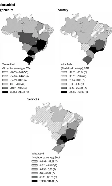
Table A2 in the appendix shows the evolution of value added (VA), la-bor (L) and capital (K) at the national level and some descriptive statistics. The high values of the standard errors reveal the great diversity across regions in each sector. Figure 1 exhibits maps displaying value added, labor and capital levels by states in 2014, the last year of our period of analysis, measured in relation to the national average. With few exceptions, it is clear that the Southeastern and Southern states concentrate the economic activity of the country in all sectors.
Table A3 in the appendix details the annual average of labor productiv-ity by state and sector. Shaded cells are states with an above-average labor productivity. This happens mostly in the states of the Southeast, South and Center-West to agriculture and services and Southeast and South to industry. Bahia and Amazonas are the only ones to have above-average labor productivity in industry outside those regions and Rondônia, Acre and Tocantins to agriculture.
from year to year replicate the oscillations in sales observed in each state. From 2006 on, we simply added to the observed stock in 2006 the state annual sales reported by Anfavea. The possibility that tractors could be sold in one state and used in another state is not a problem in the period 1996-2006, since the methodology makes sure the stocks in each state are ex-actly those reported in the censuses. From 2007 on, this could be a problem. However, the effi ciency results would be biased only if some states had systematic tractor trade defi cits and others, superavits. Our analysis of the period within censuses indicates that the problem is not important, but we really do not have ways to access how serious of a problem this could be from 2007 on. In any case, we found no better alternative to generating state level series of capital stocks in agriculture.
12 Several empirical tests were made using different measures of capital for each sector before choosing the best model. For instance, energy consumption was also considered for agriculture and services, but it led to poorer results. According to Arbache (2015), who in-vestigated productivity in the Brazilian service sector between 1998 and 2001, 89% of the fi rms have from 0 to 10 employees. The subsector of surveillance, security and valuable transportation is the largest in terms of number of employees. This is why we used state fuel consumption to distribute energy consumption in the service sector. Not only did this mean we had consistent data, but also better results.
Figure 1 Value added, labor and capital across states, 2014
Agriculture
Value added
-96,93 - -82,22 (7) (% relative to average), 2014 Value Added
-63,96 - 0,00 (7)
63,05 - 173,09 (2) -82,21 - -63,97 (7)
0,01 - 63,04 (2)
173,10 - 941,84 (2)
Industry
Services
-96,55 - -84,07 (5) (% relative to average), 2014 Value Added
-64,59 - 0,00 (6)
70,07 - 193,52 (3) -84,06 - -64,60 (6)
0,01 - 70,06 (4)
193,53 - 249,38 (3)
-99,63 - -93,24 (6) (% relative to average), 2014 Value Added
-71,64 - 0,00 (7)
66,44 - 255,84 (2) -93,23 - -71,65 (7)
0,01 - 66,43 (3)
-99,25 - -89,17 (5) (% relative to average), 2014 Labor
-71,05 - 0,00 (7)
84,45 - 160,30 (3) -89,16 - -71,06 (7)
0,01 - 84,44 (3)
160,31 - 691,62 (2)
-95,34 - -74,30 (6) (% relative to average), 2014 Labor
-56,79 - 0,00 (6)
42,63 - 159,54 (3) -74,29 - -56,80 (6)
0,01 - 42,62 (3)
159,55 - 596,78 (3) -94,29 - -72,84 (5)
(% relative to average), 2014 Labor
-42,92 - 0,00 (6)
63,78 - 87,70 (3) -72,83 - -42,93 (6)
0,01 - 63,77 (4)
87,71 - 235,91 (3)
Agriculture
Labor
Industry
Source: Elaborated by the authors with data from IBGE, Ministry of Mines and Energy and Anfavea.
-99,87 - -92,90 (5) (% relative to average), 2014 Capital
-80,13 - 0,00 (7)
89,93 - 245,04 (3) -92,89 - -80,14 (7)
0,01 - 89,92 (3)
245,05 - 502,08 (2)
-99,26 - -94,31 (6)
-94,71 - -72,31 (6)
(% relative to average), 2014
(% relative to average), 2014 Capital
Capital
-75,70 - 0,00 (6)
-54,61 - 0,00 (7)
35,92 - 235,81 (3)
44,17 - 177,34 (3)
-94,30 - -75,71 (6)
-72,30 - -54,62 (6)
0,01 - 35,91 (3)
0,01 - 44,16 (3)
235,82 - 561,45 (3)
177,35 - 619,05 (2)
Agriculture
Capital
Industry
5
Results
5.1 National
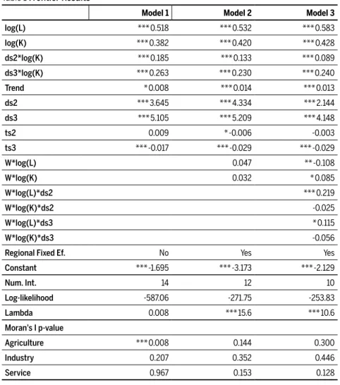
Table 1 reports the estimated Cobb-Douglas production function frontiers. The fi rst model includes labor and capital as inputs and a trend effect, to account for national macroeconomic shocks in the economy. Given that we use different proxies for capital across sectors, we have inserted
sec-toral dummies interacting with capital.14 We also differentiate productivity
levels and trends by interacting with the sectoral intercept dummies for industry and services. As such, the general productivity level and trend refers to agriculture; the productivity levels and trends for industry and services are given by adding the respective sectoral dummy coeffi cients to
the general coeffi cient.15
As the results from Model 1 show, the coeffi cients of labor and capital are signifi cant, with the expected signs and values. The positive and sig-nifi cant trend coeffi cient indicates the expansion of the agricultural fron-tier through time. The trend for industry is similar to that of agriculture, and the trend for services is signifi cantly lower. The signifi cant sectoral intercepts (ds2 and ds3) indicate that industry and services present larger
productivity levels, as compared to agriculture (constant term).16
The residual test for spatial autocorrelation using Moran’s I statistic in-dicates the presence of spatial autocorrelation. Therefore, we added re-gional fi xed effects through intercept dummies to account for unobserv-able and constant regional effects. We also include two spatial controls as independent variables, as in a SLX spatial model, interacting each input with an inverse distance spatial weight matrix (Model 2). There is no spa-tial autocorrelation in the residuals of this model, but the spaspa-tial controls
14 “2” refers to industry and “3” to services.
15 In production functions, the constant term is an estimate of the general productivity level. If we had no intercept dummies in the model, the constant would represent the average pro-ductivity level for all sectors. By including sectoral intercept dummies, we differentiate the productivity level of each sector. As explained for the sectoral trend, when the dummies for industry and services are both zero, the constant represents the productivity in agriculture. The productivity level for industry is given by the sum of the industry dummy coeffi cient and the constant. The same goes for services.
were not signifi cant. Since Model 1 indicated spatial autocorrelation for agriculture, we differentiate the spatial effects sector by sector (Model 3). The coeffi cients of interest are not substantively different from those in Models 1 and 2. In Model 3, the general trend coeffi cient indicates that effi ciency in agriculture is growing (1.3% per year); the estimated trend for industry, although with a negative coeffi cient (-0.3% per year), is not statistically different from that of agriculture. The trend coeffi cient for ser-vices is signifi cantly lower that for agriculture, and shows a negative value (1.3% – 2.9% = -1.6%).
The results indicate that a 1% increase in labor causes an increase of 0.58% in output. An increase of 1% in capital leads to an increase of 0.67% in output for services (0.428 + 0.240), 0.52% for industry (0.428 + 0.089) and 0.43% for agriculture (0.428). This is our preferred speci-fi cation and it will be the one employed in the subsequent regional and sectoral analysis. The intercept dummies for the sectors (ds2 and ds3) indicate that the annual average levels of productivity for industry
and services are higher than that of agriculture.17 However, the frontier
for agriculture expands at a faster pace compared to the other sectors (although the difference to industry is not signifi cant). This suggests a sort of productive convergence within sectors. The general trend coeffi cient indicates that agriculture experienced the strongest productivity growth in the period, 1.3% per year.
A direct comparison of our results with those presented by other stud-ies is not straightforward. We use both capital and labor as inputs, while the majority of analyses are based on a partial concept of productivity, value added per worker. Moreover, we use state-level data to estimate the national results, which is distinct from the majority of the studies revised. Another source of diffi culty is the fact that we estimate the three sectors simultaneously, while all of the studies reviewed produce estimates for individual sectors. A fourth issue lays on the periods considered, which do not match ours. In spite of these methodological differences, our results are in line with the main fi ndings of those studies at the national level.
The results for agriculture are compatible, in general terms, with the lit-erature presented in the introduction. Gasques et al. (2014), estimating TFP
using only data on agriculture, indicate a higher growth rate in the period 2000-2012, but the results point in the same direction as ours.
Table 1 Frontier Results
Model 1 Model 2 Model 3
log(L) *** 0.518 *** 0.532 *** 0.583
log(K) *** 0.382 *** 0.420 *** 0.428
ds2*log(K) *** 0.185 *** 0.133 *** 0.089
ds3*log(K) *** 0.263 *** 0.230 *** 0.240
Trend * 0.008 *** 0.014 *** 0.013
ds2 *** 3.645 *** 4.334 *** 2.144
ds3 *** 5.105 *** 5.209 *** 4.148
ts2 0.009 * -0.006 -0.003
ts3 *** -0.017 *** -0.029 *** -0.029
W*log(L) 0.047 ** -0.108
W*log(K) 0.032 * 0.085
W*log(L)*ds2 *** 0.219
W*log(K)*ds2 -0.025
W*log(L)*ds3 * 0.115
W*log(K)*ds3 -0.056
Regional Fixed Ef. No Yes Yes
Constant *** -1.695 *** -3.173 *** -2.129
Num. Int. 14 12 10
Log-likelihood -587.06 -271.75 -253.83
Lambda 0.008 *** 15.6 *** 10.6
Moran's I p-value
Agriculture *** 0.008 0.144 0.300
Industry 0.207 0.352 0.446
Service 0.967 0.153 0.128
*, ** and *** signifi cant at 10%, 5% and 1%, respectively.
Source: Elaborated by the authors.
(2013) indicate declining productivity in manufacturing, especially in low-tech sectors, but their period of analysis is 1996-2007.
Productivity in services declined at 1.6% per year, which is compatible with the fi ndings of Arbache (2015) and Jacinto and Ribeiro (2015).
Thus, our national results, which are based on regional data, are con-sistent with the results obtained in studies developed with national data, giving us confi dence to proceed with the regional analysis.
5.2 Regional
5.2.1 Effi ciency Levels
The model produces effi ciency level indicators for each state, by year and by sector. Table 2 presents the ranking of states in terms of the average of effi ciency in the whole period. The continuous horizontal line positions the states in terms of the national average; the dotted lines indicate the top, middle and lower thirds. The sectoral average is reported at the bot-tom of the table.
Table 2 Estimated Effi ciency Levels (average 2000-2014)
Rank Agriculture Industry Services Aggregate
State Effi ciency State Effi ciency State Effi ciency State Effi ciency
1 MG 0,880 AM 0,899 DF 0,917 DF 0,899
2 MT 0,875 RS 0,892 SC 0,915 RJ 0,889
3 TO 0,869 BA 0,889 PB 0,912 SP 0,852
4 MA 0,850 SP 0,867 RN 0,906 PB 0,848
5 AC 0,847 RJ 0,860 RJ 0,900 PE 0,845
6 GO 0,844 PR 0,858 PE 0,897 CE 0,843
7 AP 0,828 PI 0,842 CE 0,893 RS 0,838
8 MS 0,798 CE 0,755 AL 0,892 RN 0,837
9 PA 0,728 SE 0,755 ES 0,888 PR 0,817
10 PR 0,727 RN 0,739 RS 0,875 AL 0,815
11 ES 0,723 PE 0,723 RR 0,859 RR 0,813
12 RO 0,704 PB 0,698 SP 0,850 SC 0,806
13 SP 0,674 MG 0,691 SE 0,840 ES 0,795
14 RR 0,670 RO 0,688 PR 0,816 SE 0,783
15 PB 0,644 AL 0,676 PI 0,810 PI 0,764
16 CE 0,601 ES 0,662 MA 0,698 MA 0,717
17 AL 0,586 SC 0,659 PA 0,693 MS 0,704
18 SC 0,575 TO 0,656 MS 0,679 MG 0,692
19 PE 0,559 DF 0,638 MG 0,654 TO 0,674
20 RS 0,531 MS 0,616 TO 0,557 PA 0,653
21 RN 0,481 AP 0,598 AP 0,476 MT 0,587
22 RJ 0,456 MT 0,565 GO 0,475 AC 0,565
23 AM 0,455 PA 0,556 BA 0,470 GO 0,561
24 PI 0,433 GO 0,549 AC 0,432 AM 0,559
25 BA 0,389 MA 0,516 RO 0,424 BA 0,555
26 SE 0,337 RR 0,486 MT 0,382 RO 0,545
27 DF 0,264 AC 0,358 AM 0,241 AP 0,513
Average 0,642 0,692 0,717 0,732
Source: Elaborated by the authors.
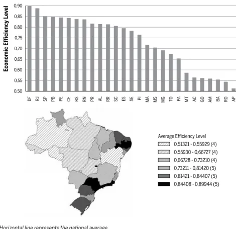
results are displayed in Figure 2. The top performer is DF, due to its top position in services, its most relevant activity. SP and RJ, which constitute the manufacturing core of the country’s economy, come next. Other tradi-tional industrialized states from the South are also in this group (RS, PR). Good performance in services granted four states from the poor Northeast region (PB, PE, CE, RN) a position in the upper tier of aggregated effi ciency.
Figure 2 Aggregate Estimates of Regional Effi ciency Levels
Horizontal line represents the national average.
Source: Elaborated by the authors.
5.2.2 Effi ciency Growth
The model provides estimates of average effi ciency growth rates for each state and sector in the period. The results are presented in Table 3.
0,51321 - 0,55929 (4) Average Effi ciency Level
0,66728 - 0,73210 (4)
0,81421 - 0,84407 (5) 0,55930 - 0,66727 (4)
0,73211 - 0,81420 (5)
0,84408 - 0,89944 (5)
0,50 0,75
0,70
0,65
0,60
0,55 0,90
0,85
0,80
DF RJ SP PB PE CE RS RN PR AL RR SC ES SE PI MA MS MG TO PA MT AC GO AM BA RO AP
E
conomic Ef
ficiency
L
ev
The fast-growers in agricultural effi ciency include states in the Center-West and North regions (AC, AM, RO, MT and MA in the savannah part of the Northeast), where this activity leads the state’s economies, and some states in the Southeast (SP) and South (PR, RS). The impor-tant states in industrial production do not show high effi ciency growth, which is observed in non-industrialized states (with the exception of MG). Services, again, present a distinct situation, with a mix of rich and poor states in the top tier.
The results allow us important considerations. For decades, the North-east region experienced low performance indicators, while the SouthNorth-east led the high performance of the country. The numbers indicate that the Northeast continues to perform poorly in the period as a whole, but some states from Center-West and North are growing in effi ciency. All the states in the Center-West and Southeast, with the exception of Rio de Janeiro, exhibit above-average growth. Only two states in the Northeast (BA and AL) are in that situation (a petrochemical complex in BA and an ethanol and sugar complex in AL). Despite the high level of effi ciency in services, states in that area have lost effi ciency through time.
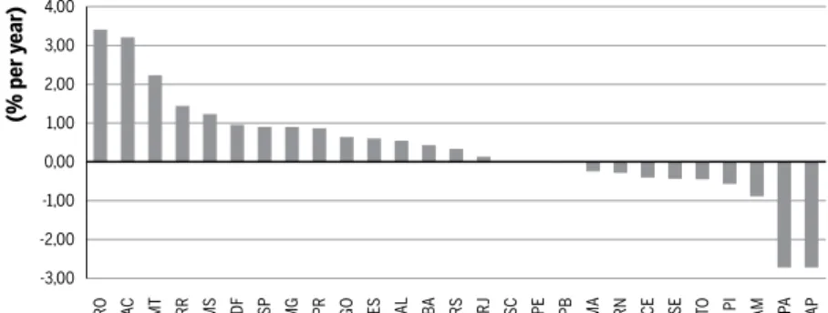
The aggregate rates presented in Table 3 are the weighted average of the sectoral rates, using the sectoral participation in the state’s value added as weights. The top fi ve growth rates are awarded to states which do not belong to the main economic core of the country, in spatial terms. States in this area come after, with growth rates much smaller than that of the fi rst group. At the other end of the distribution, only states in the Northeast and North regions belong to the group with low growth rates.
Few states actually have rates above the national average, and these are concentrated in the southern regions. Only nine states present positive ef-fi ciency growth in all sectors (RO, AC, BA, RJ, PR, RS, MT, MS and DF). PA is the only with negative rates in all sectors.
poor Northeast region, poor performance is observed in all sectors, but typically agriculture shows the worst performance in this region, followed by services. Figure 3 shows the rank of the growth rates of aggregate ef-fi ciency for the states.
Table 3 Effi ciency Annual Growth Rates (2000-2014)
Rank Agriculture Industry Services Aggregate
State Effi ciency State Effi ciency State Effi ciency State Effi ciency
1 SP 4,49 MT 6,54 RR 2,61 AC 3,41
2 AC 3,83 RO 6,46 RO 2,27 RO 3,21
3 AM 3,39 AC 4,04 AC 2,13 MT 2,23
4 RO 3,02 GO 3,89 ES 1,73 RR 1,44
5 PR 3,01 MS 3,65 MT 1,61 MS 1,23
6 RN 2,52 PE 3,14 MS 1,32 DF 0,96
7 MA 1,92 MG 1,66 SP 1,24 SP 0,90
8 RS 1,92 PB 1,58 MG 1,18 MG 0,90
9 MT 1,9 RN 1,48 BA 0,98 PR 0,869
10 DF 1,82 CE 1,44 DF 0,94 GO 0,64
11 GO 1,80 RR 1,22 AL 0,83 ES 0,61
12 TO 1,50 SC 0,95 PR 0,62 AL 0,55
13 AP 0,66 DF 0,93 RS 0,47 BA 0,43
14 BA 0,62 RJ 0,80 RJ 0,04 RS 0,34
15 SE 0,61 PI 0,77 PB -0,33 RJ 0,14
16 RJ 0,37 PR 0,72 SE -0,34 SC 0,00
17 MS 0,17 TO 0,67 SC -0,45 PE 0,00
18 MG -0,76 AL 0,38 PE -0,64 PB -0,019
19 ES -1,19 BA 0,07 MA -0,70 MA -0,24
20 AL -1,70 RS 0,05 CE -0,77 RN -0,28
21 PE -2,38 AM -0,11 RN -0,83 CE -0,40
22 PB -2,80 SP -0,27 PI -0,90 SE -0,44
23 CE -3,02 ES -0,41 GO -0,95 TO -0,45
24 SC -3,14 SE -0,96 AM -1,77 PI -0,57
25 RR -4,23 AP -1,78 TO -1,83 AM -0,89
26 PA -4,64 PA -2,81 PA -2,06 PA -2,72
27 PI -4,73 MA -4,14 AP -3,07 AP -2,72
Average 0,18 1,11 0,12 0,34
Figure 3 Aggregate Estimates of Regional Effi ciency Growth Rates (% per year)
Source: Elaborated by the authors.
Again, a comparison of these results with those produced by other authors is plagued by the diffi culties pointed out earlier. Gasques et al. (2013) es-timated TFP in agriculture in the period 2000-2012 for some states, using labor, land and capital as inputs. They found that MG, BA, GO, PR and MT presented above-average TFP growth rates. These states are in the above-average group also in our study, but only PR and MT are in our top-growing group. In industry, Britto et al. (2015) considered the period 1996-2011, using a partial productivity indicator (VA/L). They found negative growth rates for all macro regions, but the Center-West and the Northeast presented better performance. AM and PA are in the lower tier of our results, a result in line with their fi nding that the North macro region had the most intensive decrease in productivity. The states of MT, GO and MS are in our upper tier, which is compatible with their result for the
Center--3,00 2,00
1,00
0,00
-1,00
-2,00 3,00 4,00
AC
RO MT RR MS DF SP MG PR GO ES AL BA RS RJ SC PE PB MA RN CE SE TO PI AM PA AP
E
conomic Ef
ficiency
Gr
o
w
th R
ate
(%
per y
ear
)
-2,72 - -0,45 (5) Annual Average Growth Rate (%)
0,00 - 0,43 (5)
0,88 - 1,23 (4) -0,44 - -0,01 (5)
0,44 - 0,87 (4)
West macro region. Their conclusion that the Northeast macro region had better-than-average performance is not contradicted by our fi nding that PE, PB, RN and CE are in the upper tier of productivity growth. In spite of the differences in methodology and periodicity, our regional results, in general, are in line with the available evidence.
6
Regional effi ciency convergence
As mentioned before, some effi ciency results are compatible with the re-gional disparity levels observed in the country in many aspects, as GDP per capita, poverty, education, as well as in regional concentration. Chang-ing this situation requires that low performChang-ing regions improve at a faster rate than high performing regions. The presence of convergence indicates that differences in productivity levels across states will reduce over time. This could happen both at a national upper or lower level, depending on the national trend. If productivity is growing at the national level, as is the case of agriculture, the resulting equality will occur at a higher level of productivity. In the case of services, which show declining productivity, equality would happen at a lower effi ciency level.
In order to analyze signs of convergence in each sector, we have cor-related the initial (average of 2000-2002) levels of effi ciency in each state with the estimated effi ciency growth rates, as presented in Figure 4 to 7.
Figure 4 Regional Effi ciency Levels and Growth Rates in Agriculture
Source: Elaborated by the authors.
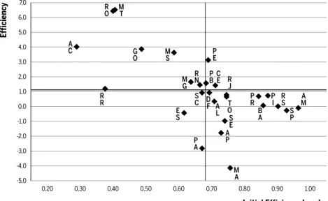
The situation with industry (Figure 5) is closer to convergence, since states with low initial effi ciency levels tend to present higher growth rates, and states at the other extreme, negative rates. AM, home of the free import zone, was the most effi cient in industry, and depicted a negative growth rate. In the same region, AP also presented a negative growth rate. The up-per left-hand quadrant receives northern (RO, AC, RR) and center-western states (MT, MS, GO), which, together with the northeastern state of RN and southeastern state of MG, show below-average initial levels and posi-tive growth rates. The economically important states of the rich South-east (RJ, SP) and South (RS, PR, SC) show above-average initial levels and negative growth rates. A simple regression of the growth rates on the ini-tial levels (2000-2002 average) indicates that, at the 1% signifi cance level, convergence cannot be ruled out. As can be seen in Figure 5, the most representative states in terms of industrial production are in the fourth quadrant, meaning high effi ciency levels and negative growth rates. Thus, the ending result of the convergence process comes with a decrease in the national effi ciency level.
S P A C M A S C P B C E P A R R M G A L M S G O P E P I R J B A S E D F R N R S A M E S A P T O P R R O M T
Initial Efficiency Level
-6,0 -1,0 -2,0 -3,0 -4,0 -5,0 0,0 4,0 3,0 2,0 5,0 1,0 Ef ficiency
0,30 0,40 0,50
Figure 5 Regional Effi ciency Levels and Growth Rates in Industry
Source: Elaborated by the authors.
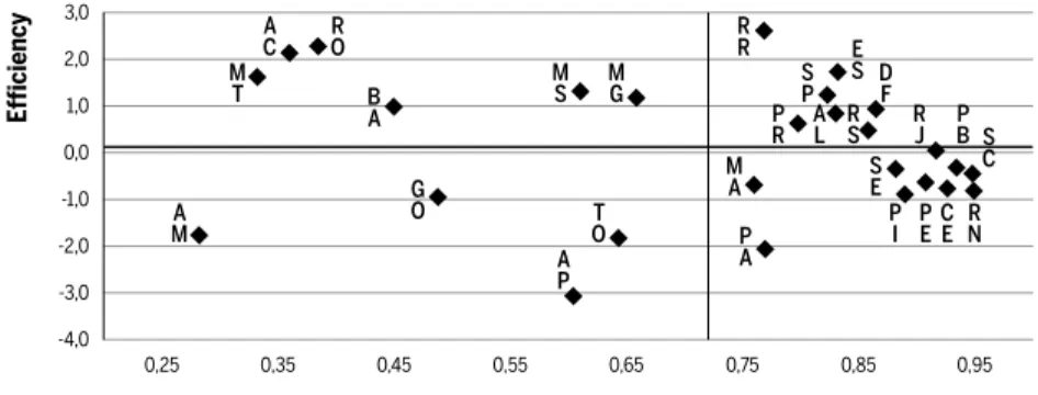
The heterogeneous service sector is more complex to analyze (Figure 6). Of the 17 states with above-average initial effi ciency levels, seven present-ed positive, and ten negative growth rates. The same proportion (60/40) situation is repeated with the below-average states. All the four negative cases of low levels and negative rates belong to the northern region, and GO, in the Center-West, but some positive cases are also from those re-gions (RO, AC, MT, MS). A simple regression of the growth rates on the initial levels (2000-2002 average) did not indicate signs of convergence.
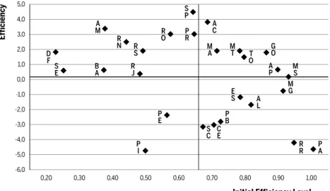
Considering the aggregate of all sectors, displayed in Figure 7, it seems that some convergence is taking place. The northern states of RO, AC and MT display low average initial effi ciency levels, but experienced the highest effi ciency growth rates. However, AP and AM, in the same re-gion, with similar average initial effi ciency, presented negative effi ciency growth rates. States in the right-hand side of the horizontal axis display above-average initial effi ciency levels. In this case, we observe more states presenting negative growth rates. Seven out of the nine northeastern states showed negative effi ciency growth rates. A simple regression of the growth rates on the initial levels (2000-2002 average) indicates that con-vergence cannot be ruled out at the 10% signifi cance level. These results
P I P E M T M A A P A L C E R J S E D
F OT
A M S P B A R S P R E S R R M G M S G O R O A C R N S C P A
Initial Efficiency Level
P B -4,0 1,0 0,0 -1,0 -2,0 -3,0 -5,0 2,0 6,0 5,0 4,0 7,0 3,0 Ef ficiency
0,30 0,40 0,50
are compatible with Azzoni and Silveira-Neto (2005), who, in spite of the difference in period of analysis, concluded that agriculture and services acted in favor of divergence, while industry (especially manufacturing) fa-vored the convergence.
Figure 6 Regional Effi ciency Levels and Growth Rates in Services
Source: Elaborated by the authors.
Figure 7 Regional Effi ciency Levels and Growth Rates – All Sectors
Source: Elaborated by the authors.
7
Conclusions
We have tackled the question of regional inequalities in Brazil from the fundamental point of view of the evolution of regional competitiveness. We have estimated effi ciency levels and growth for the states in recent
D F E S R R R O R N M A P A S E P I R S S P A L P R B A A C M
T MS MG
G O A P T O A M
Initial Efficiency Level
C E R
J PB S
C P E -3,0 2,0 1,0 0,0 -1,0 -2,0 -4,0 3,0 Ef ficiency
0,35 0,45 0,55
0,25 0,65 0,75 0,85 0,95
Initial Efficiency Level
P B P E R S D F S P S C A L M S A M A P G
O RJ
C E P I P A M A T O M G E S R
R PR
S E A C R O M T B A R N -2,0 3,0 2,0 1,0 0,0 -1,0 -3,0 4,0 Ef ficiency
years, in order to gather information on their relative positions and the evolution of productivity, as a sign of potential future competitiveness. We use state-level data for the fi rst time in this type of estimative proce-dure. Our results show that agriculture is leading the growth in effi ciency at the national level, followed by industry, probably due to the extrac-tive activities. The tertiary sector experiences a decrease in productivity. These aggregate results are compatible with the available estimates based on national data. Thus, our approach provides regional estimates that are compatible with the established national results.
Other contributions of this study relate to the simultaneous estimation of effi ciency for the three main sectors of activity. Other authors have estimated similar measures for individual sectors, ignoring the interaction between sectors of activity. By dealing with a period already into the XXI century, we provide evidence on the possible effects of important changes in the national economy. We use Stochastic Frontiers to estimate the ef-fi ciency levels, introducing spatial effects in the estimations, which is new in the literature of both topics.
as automobile assembling plants in Bahia and Recife, the naval industry and a massive petrochemical complex in Recife. Since these factors
ex-erted their infl uence mostly in the 21st Century, their consequences might
only be starting to appear in the most recent trends.
The recent changes are good news, in terms of the excessive concentra-tion of producconcentra-tion in the country, as well as in terms of regional inequal-ity indicators. But the changes are too soft to produce relevant changes in the highly concentrated situation observed in the country. Even after two decades of a stabilized and more open economy, the competitive-ness situation still, on average, favors the traditional economic core. In spite of the recent progress, the competitive position of peripheral regions is limited by the lack of infrastructure, especially in comparison to the core region (Schettini; Azzoni, 2015). The maintenance of the scenario of high demand for wage goods, propelled by social programs and the imple-mentation of large scale projects, could increase the stress on the limited infrastructure present outside the core region. Surpassing this barrier is a challenge to government, which is locked into a tight budgetary situa-tion. Creative ways of fi nancing infrastructure expansion will have to be designed and implemented, with the necessary participation of the private sector. But the positively changing scenario might make investments in infrastructure in the peripheral regions more attractive to private investors, provided a clean and safe regulatory apparatus is established. Maybe the challenge lies in providing such apparatus in a sound way.
References
AIGNER, D.J.; LOVELL, C.A.K; SCHMIDT, P. Formulation and Estimation of Stochastic Frontier Production Function Models. Journal of Econometrics, v. 6, p. 21-37, 1977.
ANSELIN, L. Spatial Econometrics: Methods and Models. Netherlands: Springer, 1988.
ARBACHE, J. Produtividade no Setor de Serviços. In: DE NEGRI, F.; CAVALCANTE, L.R. (Ed.). Produtividade no Brasil: Desempenho e Determinantes – V2. Brasília: IPEA, 2015. AZZONI, C.R.; HADDAD, E.A. Regional Disparities. In: BAER, W.; AZZONI, C.R.;
AMMAN, E. (Ed.). The Oxford Handbook of the Brazilian Economy. USA: Oxford University Press, 2018.
BAER, W. The Brazilian Economy: Growth and Development. USA: Lynne Rienner Publishers, 6th Edition, 2007.
BALK, B.M. Scale Effi ciency and Productivity Change. Journal of Productivity Analysis, v. 15, n. 3, p. 159-183, 2001.
BARBOSA FILHO, F.H.; PESSÔA, S.A.; VELOSO, F.A. Evolução da Produtividade Total dos Fatores na Economia Brasileira com Ênfase no Capital Humano – 1992-2007. Revista Bra-sileira de Economia, v. 64, n. 2, p. 91-113, 2010.
BARRETO, F.A.F.D.; NOGUEIRA, C.A.G.; ROSA, A.L.T. Crescimento e Capital Huma-no: Evidências Empíricas Recentes para o Brasil numa Perspectiva Regional. Texto para Discussão, Fortaleza, CAEN/UFC, 1999.
BONELLI, R. Growth and productivity in Brazilian industries: Impacts of Trade Orientation. Journal of Development Economics, v. 39, n. 1, p. 85-109, 1992.
BONELLI, R. Ensaios sobre política econômica e industrialização no Brasil. Rio de Janeiro: Senai--DN/DITEC/DPEA, 1996.
BONELLI, R. Produtividade e Armadilha do Lento Crescimento. In: DE NEGRI, F.; CAVAL-CANTE, L.R. (Ed.). Produtividade no Brasil: Desempenho e Determinantes – V1. Brasília: IPEA, 2014.
BONELLI, R.; FONSECA, R. Ganhos de Produtividade e de Efi ciência: Novos Resultados para a Economia Brasileira. Pesquisa e Planejamento Econômico, v. 28, n. 2, p. 273-314, Aug. 1998. BONELLI, R.; BACHA, E.L. Crescimento brasileiro revisitado. In: VELOSO, F. et al. (ed.).
De-senvolvimento Econômico: uma Perspectiva Brasileira. Rio de Janeiro: Elsevier, 2013.
BONELLI, R.; VELOSO, F. Rio de Janeiro: Crescimento Econômico e Mudança Estrutural. In: PINHEIRO, A. C.; VELOSO, F. (Ed.). Rio de Janeiro: um estado em transição. Rio de Janeiro: Editora FGV, 2012.
BRAGAGNOLO, C.; SPOLADOR, H.F.S.; BARROS, G.S.C. Regional Brazilian Agriculture TFP Analysis: A Stochastic Frontier Analysis Approach. EconomiA, Brasília, v. 11, n. 4, p. 217–242, 2010.
BRIGATTE, H.; TEIXEIRA, E.C. Determinantes de longo prazo do produto e da produtivida-de total dos fatores da agropecuária brasileira no período 1974-2005. Revista produtivida-de Economia e Sociologia Rural, Piracicaba, SP, v. 49, n. 04, p. 815-836, 2012.
BRITTO, G.; AMARAL, P.V.; ALENCAR, D.A. Produtividade industrial nas microrregiões brasileiras (1996-2011). In: DE NEGRI, F.; CAVALCANTE, L.R. (Ed.). Produtividade no Brasil: Desempenho e Determinantes – V2. Brasília: IPEA, 2015.
CANGUSSU, R.C.; SALVATO, M.A.; NAKABASHI, L. Uma análise do capital humano so-bre o nível de renda dos estados brasileiros: Mrw versus mincer. Estudos Econômicos, v. 1, n. 40, p. 153-183, 2010.
DE NEGRI, F.; CAVALCANTE, L.R. Os dilemas e os desafi os da produtividade no Brasil. In: DE NEGRI, F.; CAVALCANTE, L.R. (Ed.). Produtividade no Brasil: Desempenho e Determi-nantes – V1. Brasília: IPEA, 2014.
FARREL, M.G. The Measurement of Productive Effi ciency. Journal of the Royal Statistical Society, v. 120 (Series A), n. 3, p. 253-281, 1957.
FEIJÓ, C.A.; CARVALHO, P.G.M. Uma Interpretação sobre a Evolução da Produtividade Industrial no Brasil nos Anos Noventa e as “Leis” de Kaldor. Nova Economia, v. 12, n. 2, p. 57-78, 2002.
FELEMA J.; RAIHER, A.P.; FERREIRA, C.R. Agropecuária Brasileira: Desempenho Regional e Determinantes de Produtividade. Revista de Economia e Sociologia Rural, Piracicaba, SP, v. 51, n. 3, p. 555-574, 2013.
FERREIRA, F.H.G.; LEITE, P.G.; LITCHFIELD, J.A. The Rise and Fall of Brazilian Inequality: 1981-2004. Working Paper 3867, Washington, D.C.: World Bank, 2006.
FERREIRA, P.C.; VELOSO, F. O Desenvolvimento Econômico Brasileiro no Pós-Guerra. In: VELOSO, F. et al. (Ed.). Desenvolvimento Econômico: uma Perspectiva Brasileira. Rio de Janeiro, Elsevier, 2013.
FIGUEREDO, L.; NORONHA, K.; ANDRADE, M. Os Impactos da Saúde Sobre o Cresci-mento Econômico na Década de 90: Uma Análise para os Estados Brasileiros. Texto para discussão 219, Cedeplar/UFMG, 2003.
FRANZESE, R.; HAYS, J. Spatial-Econometric Models of Cross-Sectional Interdependence in Political-Science Panel and Time-Series-Cross-Section Data. Political Analysis, v. 15, n. 2, p. 140-164, 2007.
GALEANO, E.A.V; FEIJÓ, C. A estagnação da produtividade do trabalho na indústria brasi-leira nos anos 1996-2007: análise nacional, regional e setorial. Nova Economia, v. 23, n. 1, p. 9-49, 2013.
GALEANO, E.A.V.; WANDERLEY, L.A. Um estudo sobre o comportamento da produtivida-de industrial do trabalho nas regiões do Brasil no período produtivida-de 1996 a 2010. Revista Geogra-fares, n. 15, p. 139-180, 2013.
GALLO, J.L.; DALL’ERBA, S. Spatial and Sectoral Productivity Convergence Between Euro-pean Regions, 1975-2000. Papers in Regional Science, v. 87, n. 4, p. 505-525, 2008. GASQUES, J.G.; CONCEIÇÃO, J.C.P.R. Transformações Estruturais da Agricultura e
Produti-vidade Total de Fatores. Texto para Discussão N. 768, IPEA Brasília, 2000.
GASQUES, J.G.; BASTOS, E.T.; BACHI, M.R.P.; CONCEIÇÃO, J. Condicionantes da Produ-tividade da Agropecuária Brasileira. Texto para Discussão N. 1017, IPEA Brasília, p. 7-30, 2004a.
GASQUES, J.G.; REZENDE, G. C.; VERDE, C.M.V.; SALERNO, M.S., CONCEIÇÃO, J. C.P.R.; CARVALHO, J.C.S. Desempenho e crescimento do agronegócio no Brasil. Texto para Discussão N. 1009, IPEA Brasília, v. 1, p. 1-39, 2004b.
GASQUES, J.G.; BASTOS, E.T.; VALDES, C.; BACCH, M.R.P. Produtividade da Agricultura Brasileira e os Efeitos de Algumas Políticas. Revista de Política Agrícola, n. 3, p. 83-92, 2012. GASQUES, J.G.; BASTOS, E.T.; VALDES, C.; BACCHI, M. Produtividade e Crescimento:
Algumas comparações. In: ALVES, E.R.A.; SOUZA, G.S.; GOMES, E.G. (Ed.). Contribuição da Embrapa para o Desenvolvimento da Agricultura no Brasil. Brasília: Embrapa. 2013. GASQUES, J. G.; BASTOS, E.T.; VALDES C.; BACCHI, M. Produtividade da agricultura
p. 87-98, Jul/Ago/Set 2014.
GOMES, V.; PESSÔA, S.; VELOSO, F. Evolução da produtividade total dos fatores na eco-nomia brasileira: uma análise comparativa. Pesquisa e Planejamento Econômico, v. 33, n. 3, p. 389-434, 2003.
GONÇALVES, S.P.; NEVES, E.M. Inovação tecnológica, produtividade e preço ao consumidor de feijão no estado de São Paulo, 1970-2005. In: XLV CONGRESSO DA SOBER, Londri-na: UEL, 2007.
GRAY, E.; JACKSON, T.; ZHAO, S. Agricultural Productivity: Concepts, Measurement and Factors Driving It - A Perspective From the ABARES Productivity Analyses. Australia: Australian Gov-ernment Rural Industries Research and Development Corporation, n. 10/161, Mar. 2011. GREENE, W. Fixed and Random Effects in Stochastic Frontier Models. Journal of Productivity
Analysis, v. 23, n. 1, p. 7-32, 2004a.
GREENE, W. Distinguishing Between Heterogeneity and Ineffi ciency: Stochastic Frontier Analysis of 152 the World Health Organization’s Panel Data on National Health Care Systems. Health Economics, v. 13, n. 10, p. 959-980, 2004b.
IPEA. Produtividade no Brasil nos Anos 2000-2009: Análise das Contas Nacionais. Comunica-dos do Ipea, n. 133, 2012.
JACINTO, P.A.; RIBEIRO, E. P. Crescimento da Produtividade no Setor de Serviços da In-dústria no Brasil: Dinâmica e Heterogeneidade. Economia Aplicada, v. 19, n. 3, p. 401-427, 2015.
JONDROW, J.; LOVELL, C.A.K.; MATEROV, I.S.; SCHMIDT P. On the Estimation of Techni-cal Ineffi ciency in the Stochastic Frontier Production Function Model. Journal of Economet-rics, v. 19, n. 2-3, p. 233-238, 1982.
KALDOR, N. The Case for Regional Policies, Scottish Journal of Political Economy, v. 17, n. 3, p. 337-348, 1970.
KLOTZ, S. Cross Sectional Dependence in Spatial Econometric Models. Germany: Lit Verlag Mün-ster, 2004.
KUPFER, D. Trajetórias de Reestruturação da Indústria Brasileira Após a Abertura e a Estabili-zação: Temas para Debate. Boletim de Conjuntura, Rio de Janeiro, lE/UFRJ, v. 18, n. 2, 1998. LABRUNIE, M.; SABOIA, J. A produtividade do trabalho do setor de serviços e a evolução
recente do mercado de trabalho no Brasil. Texto para Discussão 026, Instituto de Economia, UFRJ, 2016.
LOVELL, C.A.K. Production frontiers and productive effi ciency. In: FRIED, H.O (Ed.) The Measurement of Productive Effi ciency: Techniques and Applications. United Kingdom: Oxford University Press, 1993
MARINHO, E.; CARVALHO, R.M. Comparações Inter-Regionais da Produtividade da Agri-cultura Brasileira - 1970-1995. Pesquisa e Planejamento Econômico, v. 34, n. 1, p. 57-92, 2004. MCMILLAN, M.S.; RODRIK, D. Globalization, Structural Change and Productivity Growth.
NBER Working Paper, n. 17143, 2011.
MESSA, A. Determinantes Da Produtividade na indústria Brasileira. In: DE NEGRI, F.; CA-VALCANTE, L.R. (Ed.). Produtividade no Brasil: Desempenho e Determinantes – V2. Brasília: IPEA, 2015.
MONASTERIO, L.; REIS, E. Mudanças na concentração espacial das ocupações nas ativida-des manufatureiras 1872-1920. Texto para Discussão N. 1361. Rio de Janeiro: Ipea, 2008. NAKABASHI, L.; SALVATO, M.A. Human Capital Quality in the Brazilian States. Revista
EconomiA, v. 8, n. 2, p. 211-229, 2007.
NORONHA, K.; FIGUEIREDO, L.; ANDRADE, M.V. Health and economic growth among the states of Brazil from 1991 to 2000. Revista Brasileira de Estudos Populacionais, v. 27, n. 2, p. 269-283, 2010.
NOGUEIRA, M.O.; INFANTE, R.; MUSSI, R. Produtividade do Trabalho e Heterogeneidade Estrutural no Brasil Contemporâneo In: DE NEGRI, F.; CAVALCANTE, L.R. (Ed.). Produti-vidade no Brasil: Desempenho e Determinantes – V1. Brasília: IPEA, 2014.
QUADROS, R.; FURTADO, A.; BERNARDES, R.C.; FRANCO, E. Padrões de inovação tec-nológica na indústria paulista comparação com os países industrializados. São Paulo em Perspectiva, v. 13, n. 1-2, p. 53-66, 1999.
ROSSI JR., J.L.; FERREIRA, P.C. Evolução da produtividade industrial brasileira e abertura comercial. Texto para Discussão N. 651, Rio de Janeiro: IPEA, 1999.
SCHETTINI, D.; AZZONI, C. R. Diferenciais Regionais de Competitividade Industrial do Brasil no século 21. Economia, Brasília, v. 14, n. 1B, p. 361-387, 2013.
SCHETTINI, D.; AZZONI, C. R. Determinantes Regionais da Produtividade Industrial: o Papel da Infraestrutura. In: DE NEGRI, F.; CAVALCANTE, L.R. (Ed.). Produtividade no Brasil: Desempenho e Determinantes – V2. Brasília: IPEA, 2015.
SILVEIRA-NETO, R.M.; AZZONI, C.R. Non-Spatial Government Policies and Regional In-come Inequality in Brazil. Regional Studies, v. 45, n. 4, p. 453-461, 2011.
SILVEIRA NETO, R.M.; AZZONI, C.R. Social Policy as Regional Policy: Market and Non-market Factors Determining Regional Inequality. Journal of Regional Science, v. 52, n.3, p. 433-450, 2012.
SOARES, S.; RIBAS, R.P.; SOARES, F.V. Focalização e Cobertura do Programa Bolsa-Família: Qual o Signifi cado dos 11 Milhões de Famílias? Texto para Discussão N. 1396, IPEA, 2009.
SQUEFF G.C. Desindustrialização em Debate: Aspectos Teóricos e Alguns Fatos Estilizados da Economia Brasileira. Radar Tecnologia, Produção e Comércio Exterior. Diretoria de Estudos e Políticas Setoriais, n. 21, p. 7-17, 2012.
VICENTE, J.R.; ANEFALOS, L.C.; CASER, D.V. Produtividade Agrícola no Brasil, 1970–1995. Agricultura em São Paulo SP, v. 39, n. 2, p. 1-23, 2001.
VICENTE, J.R. Produtividade Total de Fatores e Efi ciência no Setor de Lavouras da Agricultu-ra BAgricultu-rasileiAgricultu-ra, Revista de Economia e Agronegócio, v. 9, n. 3, p. 303-324, 2011.
VIEIRA FILHO J.E.R.; CAMPOS, A.C.; FERREIRA, C.M.C. Abordagem Alternativa do Cres-cimento Agrícola: um Modelo de Dinâmica Evolucionária. Revista Brasileira de Inovação, Campinas, v. 4, n. 2, p. 425-476, 2005.
WEBBER, D.J.; HUDSON, J.; BODDY, M.; PLUMRIDGE, A. Regional Productivity Differen-tials in England: Explaining the Gap. Papers in Regional Science, v. 88, n. 3, p. 609-621, 2009.
About the authors
Daniela Schettini - [email protected]
Instituto de Relações Internacionais - Universidade de São Paulo. Carlos Roberto Azzoni - [email protected]
Faculdade de Economia, Administração e Contabilidade - Universidade de São Paulo.
About the article
APPENDIX
Table A1 States and Regions
North (N) Northeast (NE) Southeast (SE) South (S) Center-West (CW)
RO – Rondônia
AC – Acre
AM – Amazonas
RR – Roraima PA – Pará
AP – Amapá
TO - Tocantins
MA – Maranhão
PI – Piauí
CE – Ceará
RN – Rio Grande do Norte
PB – Paraíba
PE – Pernambuco
AL – Alagoas SE – Sergipe
BA - Bahia
MG – Minas Gerais
ES – Espírito Santo
RJ – Rio de Janeiro
SP – São Paulo
PR – Paraná
SC – Santa Catarina
RS – Rio Grande
do Sul
MS – Mato Grosso
do Sul
MT – Mato Grosso GO – Goiás
DF – Distrito Federal
Table A2 Descriptive Statistics
Annual Average Std. Dev. Minimum Maximum
Agriculture
VA 21,560 (AP, 2003) 3,646,652 (MG, 2011)
801.734 850.174 21,560 (AP, 2003) 3,646,652 (MG, 2011)
L 454.057 405.812 11,639 (AP, 2001) 1,675,794 (BA, 2009)
K 30.519 45.617 41 (AP, 2014) 190,491 (RS, 2014)
Industry
VA 2.561.871 4.858.193 8,613 (AC, 2001) 27,185,702 (SP, 2008)
L 51.818 86.642 363 (RR, 2014) 477,760 (SP, 2011)
K 173.415 280.251 745 (AC, 2000) 1,546,169 (SP, 2008)
Services
VA 6.952.270 13.600.000 138,991 (RR, 2000) 99,229,751 (SP, 2014)
L 1.329.757 1.870.262 41,927 (RR, 2001) 10,835,111 (SP, 2014)
K 2.281 3.505 75 (RR, 2003) 23,921 (SP, 2014)
Figure A1 Evolution of the main variables at the national level
Value Added (Y)
BRL of 2013
10.000.000 30.000.000
20.000.000
0
Agricultur
e
2000 2001 2002 2003 2004 2005 2006 2007 2008 2009 2010 2011 2012 2013 2014
BRL of 2013
30.000.000 90.000.000
60.000.000
0
Indus
tr
y
2000 2001 2002 2003 2004 2005 2006 2007 2008 2009 2010 2011 2012 2013 2014
BRL of 2013
100.000.000 300.000.000
200.000.000
0
S
er
vice
s
Number of employees
11.000.000 13.000.000
12.000.000 14.000.000
10.000.000
Agricultur
e
2000 2001 2002 2003 2004 2005 2006 2007 2008 2009 2010 2011 2012 2013 2014
Number of employees
1.200.000 1.400.000
1.300.000 1.500.000 1.600.000
1.100.000
Indus
tr
y
2000 2001 2002 2003 2004 2005 2006 2007 2008 2009 2010 2011 2012 2013 2014
Number of employees
10.000.000 30.000.000
20.000.000 40.000.000 50.000.000
0
S
er
vice
s
2000 2001 2002 2003 2004 2005 2006 2007 2008 2009 2010 2011 2012 2013 2014
Number of tractors
800.000 900.000
850.000
750.000
Agricultur
e
2000 2001 2002 2003 2004 2005 2006 2007 2008 2009 2010 2011 2012 2013 2014
Electricity (BRL of 2013)
2.000.000 6.000.000
4.000.000
0
Indus
tr
y
2000 2001 2002 2003 2004 2005 2006 2007 2008 2009 2010 2011 2012 2013 2014
Electricity (Gwh)
25.000 75.000
50.000 100.000
0
S
er
vice
s
2000 2001 2002 2003 2004 2005 2006 2007 2008 2009 2010 2011 2012 2013 2014
Table A3 Labor productivity (R$/employee, annual average, 2000-2014) Shaded cells: above average productivity
State Agriculture Industry Services
RO 22.855 21.647 27.465
AC 26.943 13.815 28.248
AM 11.340 109.717 36.096
RR 11.566 18.815 29.883
PA 11.092 36.523 29.356
AP 12.166 27.015 29.678
TO 25.907 18.192 23.861
MA 10.068 34.800 24.866
PI 5.001 21.457 22.960
CE 6.391 21.248 26.756
RN 8.021 22.594 31.953
PB 5.932 21.348 23.622
PE 5.130 27.873 33.608
AL 7.706 16.602 28.150
SE 6.324 34.716 32.508
BA 7.442 81.134 30.140
MG 20.301 45.440 41.288
ES 19.386 48.506 46.277
RJ 15.614 83.390 60.972
SP 22.939 52.717 68.864
PR 24.357 39.829 53.022
SC 22.767 28.566 51.848
RS 24.288 38.046 50.225
MS 41.443 37.243 42.702
MT 54.063 38.387 39.936
GO 40.116 33.354 36.110
DF 18.027 33.251 72.946