Instituto Superior de Economia e Gestão

(1)

Instituto Superior de Economia e Gestão

Universidade Técnica de Lisboa

M

ESTRADO

Matemática Financeira

T

RABALHO

F

INAL DE

M

ESTRADO

Dissertação

F

ORECASTING LOSS GIVEN DEFAULT WITH THE

NEAREST NEIGHBOR ALGORITHM

T

ELMO

C

ORREIA DE

P

INA E

M

OURA

(2)

Page 2

M

ESTRADO

Matemática Financeira

T

RABALHO

F

INAL DE

M

ESTRADO

Dissertação

F

ORECASTING LOSS GIVEN DEFAULT WITH THE

NEAREST NEIGHBOR ALGORITHM

T

ELMO

C

ORREIA DE

P

INA E

M

OURA

O

RIENTAÇÃO

:

D

OUTOR

J

OÃO

A

FONSO

B

ASTOS

(3)

Page 3

Acknowledgements

This dissertation would not have been possible without the help and support of

some “nearest neighbors”.

I would like to thank the guidance, help and expertise of my supervisor, João

Afonso Bastos, not to mention is technical support and knowledge of

forecasting models.

I must also acknowledge my colleague Luís Ribeiro Chorão for his advice,

support and friendship. As we both share the interest on loss given default

forecasting, our debates and exchanges of knowledge were very fruitful.

Without his motivation and encouragement I would not have considered a

master’s degree on a quantitative field.

I must also acknowledge the CEFAGE-UE (Centro Estudos e Formação

Avançada em Gestão e Economia da Universidade de Évora) for providing me

with data.

Above all, I would like to thank my wife Cláudia for her love, personal support

and great patience at all times. As always, my parents and in-laws have given

me their support, often taking care of my beloved son when I was working on

(4)

Page 4 Abstract

(5)

Page 5 Index

1. Introduction ... 6

2. Literature review ... 7

3. Theoretical Framework ... 12

3.1 Nearest Neighbor ... 14

3.2 k-NN regression ... 15

3.3 Feature transformation ... 16

3.4 Distance metrics and dissimilarity measures ... 16

3.5 Feature selection ... 21

3.6 Local models ... 23

3.7 Evaluating predictive accuracy ... 25

4. Benchmark parametric model ... 27

5. Database description ... 28

6. k-NN algorithm for LGD forecasting ... 31

6.1 Training and test data ... 32

6.2 Dimension reduction... 33

6.2.1 Feature selection (and transformation) ... 33

6.2.2 Instance selection ... 34

6.3 Distance / dissimilarity measures ... 35

6.4 Neighborhood dimension and local models ... 35

6.5 Results ... 36

(6)

Page 6

1. Introduction

With the advanced internal ratings-based approach (A-IRB), the Basel II

Framework encourages banks to use their own internal models estimates to

calculate regulatory (and economic) capital for credit risk. Three key parameters

should be properly estimated by financial institutions in order to be compliant

with A-IRB approach: probability of default (PD) over a one-year horizon, loss

given default (LGD) and exposure at default (EAD).

LGD represents the percentage of a credit instrument exposure the financial

institution might lose in case the borrower defaults. LGD is a bounded variable

in the unit interval. Its complement represents the recovery rate.

Even before the advent of Basel II regulation, the focus of academic research

and banking practice was mainly on PD modelling. PD has been the subject of

many studies during past decades, since many banks already had rating

models for credit origination and monitoring. Additionally, for academics,

publicly default data were easily available. On the other hand, until the advent of

the new Basel Capital Accord (Basel II Accord) loss data was to scarce,

especially for private instruments (e.g. bank loans). This is the reason why most

of the published work focuses on corporate bond losses. LGD for these

instruments is typically determined by market values (resulting in market LGD or

implied market LGD), whereas bank loan LGD is based on the discounted cash

flows of a workout process: workout LGD. But even inside financial institutions,

one of the major challenges for those interested in A-IRB certification has been

the collection of reliable historical loss/recovery data. In many financial

(7)

Page 7

processes had been carried out. Outsourcing of workout activities, process data

recorded only in physical support (paper), and the absence of linkage between

the original loans and the proceeds from their collateral sales are examples of

identified limitations. Whilst PD can be modeled at the counterparty level, LGD

needs to be modeled at the facility level, which increases data collection

complexity. Despite some limitations, Basel II requirements have triggered the

publication of a vast LGD literature in recent years.

2. Literature review

Accurate LGD forecasts are important for risk-based decision making, can lead

to better capital allocation and more appropriate loan pricing, and hence result

in a competitive advantage for financial institutions. However, LGD/recovery

forecast is not an easy task and has been poorly done historically. Many

institutions still use historical empirical losses or look-up tables (combining

seniority, sector, rating class and/or collateral) as their LGD forecasts. That’s

why some banking supervisors have imposed initial LGD floors, to be gradually

relieved.

Gürtler & Hibbeln (2011) have focused their work on the identification of major

pitfalls in modelling LGD of bank loans: bias due to difference in the length of

the workout processes, and neglecting different characteristics of recovered

loans and write-offs are two of the pitfalls mentioned in their work.

Several common characteristics have been identified in LGD literature:

• Recovery (or) loss distribution is said to be bimodal (two humped), with

(8)

Page 8

Dermine & Neto de Carvalho, 2006). Hence, thinking about an average

LGD can be very misleading;

• Economic cycle affects LGD: losses are (much) higher in recessions

(Carey, 1998; Frye, 2000). Other authors, like Altman et al. (2005),

Acharya et al. (2007) and Bruche & González-Aguado (2010) which

focused on the relation between PD, LGD and the credit cycle also

observed the impact of business cycle in recovery rates;

• Credit seniority and collateral seems to have effect on losses (Asarnow &

Edwards, 1995; Carey, 1998; Gupton et al., 2000; Araten et al., 2004);

• Counterparty industry is an important determinant of LGD (Altman &

Kishore, 1996; Grossman et al, 2001; Acharya et al, 2007);

• Exposure / loan size has little effect on losses. In fact this is maybe the

most ambiguous key driver of losses. Based on datasets from U.S.

market, Asarnow & Edwards (1995) and Carty & Lieberman (1996) find

no relationship between this variable and LGD. On the other side,

Felsovalyi and Hurt (1998), posted a positive correlation between both

variables. Comparing these studies one has to consider that different

datasets have been used;

• Country-specific bankruptcy regime also explains significant different

losses (Franks et al., 2004).

Initial approaches to LGD forecast were deterministic in nature, treating

recoveries as fixed values: i.e. by the use of historical losses or look-up tables

of average losses by classes of relevant LGD determinants. This has the

drawback that the marginal effect on recoveries of each characteristic cannot be

(9)

Page 9

is that Expected Loss volatility is mainly driven by PD dynamics rather than

LGD. However, some studies (Hu & Perraudin, 2002; Altman et al., 2005;

Bruche & González-Aguado, 2010 and Acharya et al., 2007) showed empirical

evidence of positive correlation between PD and LGD. This fact suggests the

existence of systematic risk in LGD, just like in PD. Ignoring that fact can result

in substantial underestimation of economic capital (Hu & Perraudin, 2002). In

Basel II Accord this issue is addressed by the use of a “downturn LGD”. At the

very beginning of this century it was generally accepted by researchers that

more sophisticated models were needed to properly deal with the high variance

of LGD within the classes of the different drivers, and with the relationship

between LGD and macroeconomic context.

In more recent studies, the recovery rate is modeled as a random variable and

the factors influencing LGD are analysed by estimating regressions. Due to the

bounded nature of the dependent variable, the use of linear regression models

estimated by ordinary least squares - OLS (Caselli et al., 2008; Davydenko &

Franks, 2008; Bellotti & Crook, 2012) can present questionable results: first

because it does not ensure that predictions lie in the unit interval, and second

because it ignores the non-constant partial effect of explanatory variables.

Gupton & Stein (2005) developed Moody’s KMV LossCalcTM_{V2 for dynamic}

prediction of LGD. Their work was based on a dataset with 3026 facility

observations (loans, bonds and preferred stock) of 1424 default firms from

1981-2004. LGD of defaulted firms is assumed to be a beta random variable

independent for each obligor. Normalized recovery rates via a beta distribution

were modeled using a linear regression of independent variables. This type of

(10)

Page 10

of the linear regression. It was one the first studies presenting out-of-sample

and out-of-time validation measures. Results were compared to the use of

historical losses and look-up table of averages. Beta distribution has been

widely used to model variables constrained in the unit interval. With appropriate

choice of parameters it can easily represent U-shaped, J-shaped or uniform

probability density functions (p.d.f.). Giese (2006) and Bruche &

González-Aguado (2010), followed this technique often used by rating agencies

(CreditMetricsTM and KMV Portfolio ManagerTM) and took advantage of the

well-known flexibility to model LGD by a mixture of beta distributions. Also using

multivariate analysis, Dermine & Neto de Carvalho (2006) identified some

significant determinants of bank loan recovery rates: size of loan, collateral,

industry sector and age of the firm. Working with a dataset from a private

portuguese bank, consisting of 374 SME defaulted loans, they used an

econometric technique for modeling proportions, the (nonlinear) fractional

regression estimated using quasi-maximum likelihood methods (Papke &

Wooldridge,1996). Their work was, to the best of the author’s knowledge, the

first one to use workout recoveries at facility level. Bellotti & Crook (2012) built

several regression models (Tobit, decision tree, standard OLS, OLS with beta

distribution, probit and fractional logit transformation of dependent variable) for

LGD prediction based on a large sample of defaulted credit cards. The

evaluation of the different models was performed out-of-sample using k-fold

cross validation. They find that the standard OLS regression model produced

the best results in many alternatives experiments. Bastos (2010a, 2010b)

proposed a non-parametric approach of LGD modeling. Unlike parametric

(11)

Page 11

data-driven, i.e., it is derived from information provided by the dataset. As a

way to resemble look-up tables, Bastos (2010a) first suggested the use of

regression trees for LGD forecasting. Whilst look-up table partitions and

dimensions are subjectively defined by an analyst or a committee, the cells in a

regression tree are defined by the data itself. Thus, LGD estimates correspond

to the cell historical average, which enables forecasts to rely on the unit interval.

Estimation results were compared to the fractional response regression

proposed by Dermine & Neto de Carvalho (2006) (dataset was also the same

used by these authors). Shortly afterwards, with the same dataset, Bastos

(2010b) proposed another non-parametric mathematical model for LGD

estimation: artificial neural networks. It consists of a group of interconnected

processing units called “neurons”. This learning technique has been

successfully employed in several scientific domains and also in PD modeling.

Bastos (2010b) has considered a logistic activation function in the output

neuron, in order to restrain forecasts to the unit interval. Results were again

benchmarked against the fractional response regression of Papke & Wooldridge

(1996).

In the wake of Bastos (2010a, 2010b) works, this study proposes another

non-parametric technique for LGD forecasting: the nearest neighbor algorithm.

Results are benchmarked against the more “conventional” fractional response

model. The next section describes the theoretical framework behind the nearest

(12)

Page 12

3. Theoretical Framework

This section presents the theoretical framework behind the tested algorithm for

LGD forecasting. The remainder of this section focuses particularly on the

description of the nearest neighbor (NN) algorithm characteristics such as

distance/(dis)similarity metrics for neighbor identification, feature transformation

and selection, and local models. It is also presented a brief description of the

fractional response regression, the parametric model to which NN regression

results will be compared to.

Prior LGD case studies show that the probability density functions of LGD (or its

complement, the recovery rate) differ between countries, portfolios, type of

credit facility and counterparty segment. Nonparametric techniques are useful

when there is little a priori knowledge about the shape of the distribution of the

dependent variable. In these methods there is no formal structure for the

density function. On the other way, parametric models often assume density

functions that are not suitable for many real-life problems because they rarely fit

the densities actually encountered in practice.

The nearest neighbor (NN) algorithm is perhaps, at least conceptually, one of

the simplest nonparametric techniques. The NN algorithm was originally

developed for classification problems, i.e., problems with discrete-valued

functions. Then, its use was spread to continuous-valued functions: NN

regression. NN regression estimators can be used either as a stand-alone

technique or as an add-on to parametric techniques.

NN belongs to the family of Machine Learning (ML) algorithms. ML is dedicated

(13)

Page 13

data-driven. In recent years there have been incredible advances in the theory

and algorithms that form the foundations of this field. In the area of financial

services, many ML applications have been developed, for example, to detect

fraudulent credit card transactions or to estimate counterparties ability to pay

(i.e., PD). However, ML algorithms have also been applied to several distinct

problems like character recognition, language processing, robotics, image

processing, terrorist threat detection, computer security, etc. Additionally, ML

draws on concepts and results of others fields of study such as statistics,

biology, cognitive science, control theory and even philosophy.

Within ML algorithms, NN regression belongs to the classes of Supervised

Learning (rather than Unsupervised Learning), and Lazy Learning (instead of

Eager Learning). As in other ML algorithms, learning in NN regression always

involves training and testing. It is “supervised” because there is a “teacher” that

provides a category or real-valued label for instances (being an instance every

training or test example, i.e., every defaulted credit instrument presented in the

dataset). NN is also a Lazy Learning technique, since we wait for query before

generalizing, i.e. induction is delayed. A training sample is needed at run-time.

On the other hand, on Eager Learning, we first generalize before the query.

Lazy learner techniques can create many local approximations and represent

more complex functions. This kind of approach can create different

approximations to the target function for each query instance (i.e. the credit

instrument which we want to forecast LGD). As referred above, LGD p.d.f. is

often not known ex-ante. NN is a procedure that bypasses probability estimation

(14)

But after all, what is the

is quite straightforward:

instances and be

rule for classifying is

variable we want to forec

it is categorical, the labe

feature (i.e. variable) spa

regression) or the catego

contains. This is called th

The concept of NN is ve

space probably belong to

continuous-valued proble

Page 14

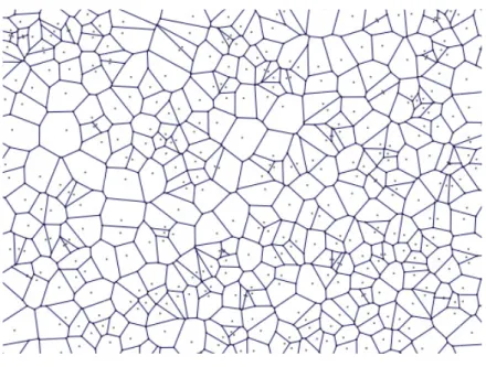
3.1 Nearest Neighbor

e nearest neighbor? The idea behind the

d: let denote a dataset

be the nearest instance to a query instan

is to assign it to the label associated

ecast is continuous (like LGD), the label is

bel is a category. This rule leads to a par

pace into Voronoi cells, each labelled by

gory (NN classification) of the instance (tr

the Voronoi tessellation of the space (see

Figure 1 – Voronoi tessellation

very easy to understand: similar patterns

to the same category or have an approxim

lems).

e concept of NN

et of labelled

nce The NN

ed with If the

is a real value, if

artitioning of the

y the value (NN

training point) it

e Figure 1).

ns in the feature

(15)

For many reasons (accu

account more than one n

neighbor (k-NN) regress

NN if we center a cell

neighbors. If the density

other hand, if density is

higher density (see Fig

whether training examp

dimensional metric spac

(dimensions).

Figur

Let us assume that we h

instances. Each instanc

instance is labelled with

estimate the query inst

Page 15

3.2 k-NN regression

curacy, variance reduction, etc) it is comm

neighbor so the technique is usually know

sion. The NN rule (1-NN) can be easily

ll about ad let it grow until it captu

ty is high near , the cell will be relatively

is low, the cell will grow large until it ent

igure 2). This algorithm assumes that

ples or query instances, could be ma

ce , where represents the number o

ure 2 – Distance to the second nearest neighbor

have a training dataset with (

ce is described by a set of features .

ith . The objective of k-NN re

stance ( target value: . G

mon to take into

own as k nearest

ly extended to

k-tures k nearest

ly small. On the

nters regions of

at all instances,

apped in a

of data features

) training

. Each training

regression is to

(16)

Page 16

instance , k-NN first locates the k nearest training

examples (the neighbors) based on some distance / dissimilarity measure

and then estimates as a function of the neighbors:

!

"

#

$ % & (1)

That is equivalent to say that, in k-NN regression, _' estimates result from local

models. In this study, is the observed LGD and _' is the predicted LGD for

each credit instrument.

3.3 Feature transformation

Before computing any distance measure we need to assure that all features are

comparable, since it is common to have features expressed in different scales.

For continuous features, two methods are often used to provide the desired

“common scale”:

• Z-score standardization: replace original value ( with

)_*+)---_,

./01 )_* (2)

• Min-Max normalization: replace original value ( with

)_*+2 )_*

203 )_* + 456 )_* (3)

where _{7 (} and _{78 (} are the minimum and maximum values of ₍

appearing in the training sample data. In Min-Max Normalization, every

normalized value will lie in the unit interval.

3.4 Distance metrics and dissimilarity measures

Like almost all clustering methods k-NN requires the use of a dissimilarity

(17)

Page 17

# # # # of instances. A metric has a formal meaning in mathematics.

Let ₍ be any set. If the function _{9 ( : (} is a metric on ₍ (and ₍ is

called a metric space) must obey to the following criteria:

• Non-negativity: # ; <

• Identity: # 0 only if #

• Symmetry: # #

• Triangle inequality: = ; # > # =

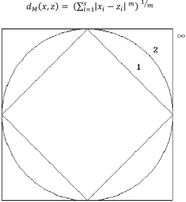
For continuous features the most common distance metrics are (input space

with features):

• Euclidean distance (? distance)

# . _" @ # (4)

It has the property of giving greater weight to larger differences on

features values.

• Manhattan or City Block distance (? distance)

# A @ # A_" (5)

? distance is also known as taxicab distance because is thought of as

the path a taxicab would take in a city (e.g. in Manhattan) between two

points.

• Chebyshev distance (? distance)

# 78 A @ # AA (6)

Chebyshev distance evaluates the maximum absolute magnitude of the

feature differences in the pair of vectors.

In Figure 3 we can see the difference between the contours of equal distance

(18)

Page 18

general distance: the Minkowski distance. The Minkowski distance of order m

is:

B # A @ # A" 2 C2 (7)

Figure 3 – Contours of equal distance for the _? (diamond), _? (circle) and _? (square) distance.

For categorical (ordinal or nominal) features, the computation of dissimilarity

measures (not always metrics) is not straightforward, since that for nominal

attributes we do not have an ordering between values. Several data-driven

(dis)similarity measures have been proposed to address this problem.

Consider a categorical data set of size N, with s categorical features/attributes,

where _D_E denotes the _&FG feature. Each attribute _D_Etake _Evalues in the given

data set.

Some common (dis)similarity measures for categorical data are:

• Hamming or edit distance

# H7IJK L DEA M # (8)

This distance does not take into account differences between the distinct

(19)

Page 19

instances will be proportional to the number of attributes in which they

(do not) match, giving the same importance to all matches and

mismatches. The per-attribute dissimilarity is {0,1} with a value of 1

occurring when there is not match, and 0 otherwise.

• Goodall measure

Goodall (1966) proposed a similarity measure for biological taxonomy

that gives greater weight to uncommon feature value matches. This

measure “normalize” the similarity between two instances by the

probability that the similarity value observed could be observed in a

random sample of two points. The behaviour of such kind of measure

directly depends on the data. Since Goodall’s original measure was

computational expensive (e.g. it accounts for dependencies between

attributes) Boriah et al. (2007) proposed a much simpler version of

Goodall similarity measure:

N # E" NE E #E (9)

with

NE E #E O

@ P QE $ E #E R

< LSTJKU J

V

and

QE $ E $_{W W @}E $ @

where _E _$ represents the number of times attribute _D_E takes the value

$ in the dataset and _X is the set of different _$ values for each attribute

(20)

Page 20

This similarity measure can be easily transformed into a dissimilarity

measure using the formula:

@ N (10)

• Inverse Occurrence Frequency (IOF)

This measure gives a lower weight to mismatches on more frequent

values.

NE E #E Y E

#E Z[\] ^_3_ :[\] ^_ `_ LSTJKU J

V

(11)

The range of _N_{E E} _#_E is _a

Zb[\]c_ded f where the minimum value is

obtained when _E and _#_Eeach occur g times and the maximum is

attained when _E and _#_E occur only once in the data set.

• Occurrence Frequency (OF)

This measure is the opposite of the IOF, i.e., it gives lower similarity

weight to mismatches on less frequent values and higher weight to

mismatches on more frequent values.

NE E #E O

E #E

Z[\]_{h_ i_}c :[\]_{h_ j_}c LSTJKU JV (12)

The range of _N_{E E} _#_E is _k

Z [\] ld _{Z [\]} dm, where the minimum value

is obtained when _E and _#_Eoccur only once in the data set, and the

maximum is attained when _E and _#_E each occur g times.

Like the Goodall measure, IOF and OF similarity measures can be

(21)

Page 21

An additional (dis)similarity measure is proposed by Gower (1971), which

permits the combination of continous and categorically valued attributes.

Mahalanobis distance (Mahalanobis, 1936) and Kullback-Leibler divergence

(Kullback & Leibler, 1951) are other popular distance measures used in

instance-base learning algorithms. Mahalanobis distance is also known as the

fully weighted Euclidean distance since it takes into account correlation

between features (through the use of a covariance matrix).

Scott (1992) and Atkeson et al. (1997) refers that the same distance metric

could be used for all feature space (global distance functions) or it can vary by

query (query-based local distance functions) or even by instance (point-based

local distance function). The scope of this work is limited to global distance

functions.

3.5 Feature selection

Feature selection is itself one of the two methods of dimension reduction. The

other method is the deletion of redundant or noisy instances in the training data,

which is designated by Instance Selection or Noise Reduction. Sometimes

instances are described by so many features and just a small subset of them is

relevant to target function. Often, the identification of nearest neighbors is easily

misled in high-dimensional metric spaces. This is known as the curse of

dimensionality and is caused by the sparseness of data scattered in space.

Identifying nearest neighbors in terms of simultaneous closeness on all features

is often not desirable. It is not probable that natural groupings will exist based

on a large set of features. Feature selection is all about selecting subset of

(22)

Page 22

each selected feature could be regulated by some weighting parameter to

include in the distance measure. In addition to accuracy (see Section 3.7)

improvement, feature selection has a big impact on computational performance.

In order to avoid the problem of high dimensionality, there are several

approaches to select or weight more heavily the most relevant features.

Cunningham & Delany (2007) divided those approaches into two broad

categories: filter approaches and wrapper methods.

Filter approaches select irrelevant features for deletion from the dataset prior to

the learning algorithm. Under this approach, feature selection is a result of

dataset analysis. Filter approaches could simply result from an expert

judgemental analysis or from the usage of a criterion to score the predictive

power of the features.

Wrapper methods make use of the k-NN algorithm itself to choose from the

initial set of features a subset of relevant ones. This methods use regression

performance to guide search in feature selection. However, if we try to test the

performance of all possible subsets of features (all combinations), wrapper

strategy becomes computationally expensive. When the number of features is

high, the two most popular techniques are:

• Forward Selection: this technique is used to evaluate features for

inclusion. Starting from an empty set, each feature is tested individually

and recorded the corresponding objective function value. The best

feature is added to the distance metric. This procedure is repeated until

some stopping criterion is met. The stopping criterion for feature

(23)

Page 23

number of features have been selected or when the gain in the objective

function is less than a pre-specified minimum change.

• Backward Selection: this technique is used to evaluate features for

exclusion. The concept is nearly the same of Forward Selection, but here

we start with the full set of features and then, at each step, exclude one

feature based on the objective function gain/loss, until the selected

stopping criterion is met.

Both wrapper techniques described above can coexist with Forced Entry,

i.e., one can force the entry of some features in the algorithm (e.g. as a

result of filter approach) and use Backward/Forward selection for the

remaining features. Feature selection is a very important step in k-NN

regression. Only relevant variables should be selected for inclusion in the

dissimilarity measure. This step also restrains variables available for local

models (e.g. Locally Weighted Regression).

3.6 Local models

In NN classification problems (instances with discrete class label), query

instance is usually labelled with the class label that occurs more frequently

among k neighbors. This procedure is known as majority voting. In this kind of

problems k should be an odd number, in order to avoid ties. In k-NN classifiers

voting could be distance weighted or not. However, in regression problems,

prediction is far more complex. Fortunately, k-NN can approximate complex

functions using local models. Atkeson & Schaal (1995) gave some examples of

possible local models: nearest neighbor (1-NN), (un)weighted average or locally

weighted regression (LWR). Nearest neighbor simply identify the closest

(24)

Page 24

model but has serious disadvantages: it is very sensitive to noisy data (e.g.

outliers) and its estimates have higher variance when compared to weighted

local models. In k-NN regression we usually want to weight nearer neighbors

more heavily than others. Weighted average local model uses all k

neighborhood instances and compute a sum of values weighted by their

distance to the query instance:

'

_*pqn*o*

n_* _

*pq (13)

where the fraction is a weighting term with sum 1. This approach was proposed

by Nadaraya (1964) and Watson (1964) and is often referred as the

Nadaraya-Watson estimator. Each neighbor weight (_U) is a kernel function of its distance

to query instance:

_U _{r b} _{e stuv t} _w (14)

The maximum value of the weighting function should be at zero distance, and

the function should decay smoothly as the distance increases. One of the most

common weighting functions is the distance raised to a negative power

(Shepard 1968):

_U _r +x (15)

In this function, _Q determines the rate of drop-off of neighbor weights with

distance. If _Q we have “pure” inverse distance weighting. When _Q increases

the weighting function goes to infinity for neighbors closer to query instance. In

the limit, we achieve exact interpolation (i.e. we achieve 1-NN), which is not

desirable for noisy data, as stated before. Among many possible weighting

functions, there is also the possibility of using un-weighted (not kernelized)

(25)

Page 25

neighborhoods, when we want to prevent distant neighbors to have very low

weights.

'

E E" (16)

In LWR, for each query, a new local model is formed to approximate . In this

statistical approach, the model is usually a weighted regression in which the

closest points (neighbors) are weighted heavier than the distant points

(neighbors). Regression is weighted because, as seen above, distance is a

measure of similarity between instances. Possible locally regressions are Linear

Function, Quadratic Function, Piecewise approximation, etc.

Remember that the predictive accuracy of local models and the overall

performance of k-NN regression depends on the neighborhood dimension (k). k

selection is a compromise between an higher value (reduces variance but can

result in the joining of neighbors with significantly different patterns/probabilities)

and a lower value (attempt to increase accuracy can be easily lead to

non-reliable estimates). In weighted local models, local outliers will be noticed if they

are close enough to the query point. Their influence will be greater in models

with weighting functions that give higher importance to closer neighbors. One

possible way for preventing their influence is eliminating them previously from

training data (in the dimension reduction stage known as Instance Selection or

Noise Reduction).

3.7 Evaluating predictive accuracy

The predictive accuracy of the models is assessed using two standard metrics,

traditionally considered: the root mean squared error and (RMSE) and the mean

(26)

Page 26

estimate differs from actual value to be estimated. Both criterions are only

applied to test sample, in order to evaluate models out-of-sample predictive

accuracy, i.e. to measure its generalization capacity. The RMSE is defined as

yzN{ k _" @ ' m | (17)

where and _~_} are the actual and predicted loss given default on loan and

is the number of loans in the test sample. The MAE is defined as

zD{ A @ ' A" (18)

The main objective is to minimize both criteria, since models with lower RMSE

and MAE can predict actual LGD more accurately. Both criteria are measures

of how well they explain a given set of observations. The major difference

between the two criteria is that RMSE, by the squaring process, gives higher

weights to larger errors. As both metrics take their values in the same range as

the error being estimated, they can be easily understood by analysts. k-NN

algorithm forecasting performance is also measured by the root relative squared

error (RRSE) and the relative absolute error (RAE), which are obtained by

measuring accuracy with respect to a simple model that always forecasts LGD

as the historical average:

yyN{ << • €*pq o*+o'* d o*+o-* d €

*pq •

+ |

yD{ << • Ao€*pq *+o'*A

Ao€*pq *+o-*A• (19)

Models with RRSE and RAE lower than 100% have better predictive accuracy

than the simple predictor. However, since IRB risk-weighted assets formulas

are very sensitive to LGD values and also because banks prefer to have

increased forecasting performance on larger risks it may be worth to consider

(27)

Page 27

consider instrument default amount as the weighting factor that indicates the

importance we wish to place on each prediction. The weighted mean absolute

error (wMAE) and the weighted root mean squared error (wRMSE) can be

computed as:

UzD{ €*pqn*Ao*+o'*A n* €

*pq UyzN{ •

n* o*+o'* d €

*pq n* €

*pq •

|

(20)

As seen before, any of these metrics can also be used to evaluate the inclusion

or exclusion of features in the model (for forward or backward selection).

Exactly the same training and test samples will be used to fit and evaluate the

accuracy of the simple one factor (historical average), nonparametric (k-NN

regression) and parametric model (fractional response regression).

4. Benchmark parametric model

In order to evaluate the relative performance of k-NN regression, a parametric

model was also fitted to data. The chosen model was the fractional response

regression (Dermine & Neto de Carvalho, 2006). Since LGD is a bounded

variable in the unit interval it is necessary an alternative nonlinear specification

to the ordinary least squares regression (OLS):

{ A‚ ƒ „…> „ > † > „E E ƒ ‚„ (21)

where _ƒ satisfies _{< ‡ ƒ # ‡} for all _# . The logistic function was

selected as the functional form of _ƒ :

ƒ ‚„ | > ˆ‰Š @‚„ (22)

Estimation was performed through the maximization of Bernoulli log likelihood

(Papke & Wooldridge, 1996) with the individual contribution given by:

(28)

Page 28

The consistency of the quasi-maximum likelihood estimator (QMLE) follows

from Gourieroux et al. (1984) since the density upon which the likelihood

function is based on is a member of the linear exponential family, and because

of the assumption that the conditional expectation of is correctly specified. In

fact, the QMLE is asymptotically normal regardless of the distribution of

conditional on _‚ .

5. Database description

The database used in this study is Moody’s Ultimate Recovery Database

(URD), which has information on US non-financial corporations. Each of the

defaulted corporations had over $50 million debt at the time of default. Moody’s

URD covers the period between 1987 and 2010 and gathers detailed

information of 4630 defaulted credit instruments (bonds and loans) from 957

different obligors. The expression “ultimate recoveries” refer to the recovery

amounts that creditors actually receive at the resolution to default, usually at the

time of emergence from bankruptcy proceedings. In the URD, Moody’s provides

three different approaches to calculating recovery, including the settlement

method, the trading price method and the liquidity event method. For each

defaulted instrument, Moody’s indicates in the URD the preferred valuation

method. This study is carried using the discounted recovery rate associated

with the recommended valuation method. For the purpose of this study, the

complement of this rate will be considered the LGD. Bonds account for almost

60 percent of defaulted instruments, while loans represent the remaining 40

percent. The average LGD on instruments included in the database is 41

(29)

Page 29

reflects the loans higher position in the obligors’ liability structure. Figure 4

shows that loan LGD distribution is strongly skewed to the left, with

approximately 65 per cent of the defaulted loans with less than 10 percent loss.

On the other side, the distribution of bond LGD appears to be bimodal and

slightly skewed to the right.

Figure 4 – LGD distribution of bonds and loans

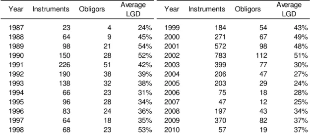
Breaking down the database by year of default we can observe that the number

of defaulted corporations increased in the early 1990s, early 2000s and again in

2008 and 2009 (Table 1). Highest LGD values are observed in 1989, 1990,

1998 and 2002.

0.00% 10.00% 20.00% 30.00% 40.00% 50.00% 60.00% 70.00%

0-0.1 0.1-0.2 0.2-0.3 0.3-0.4 0.4-0.5 0.5-0.6 0.6-0.7 0.7-0.8 0.8-0.9 0.9-1

%

c

a

s

e

s

(30)

Page 30

Table 1 – Number of instruments, obligors and average LGD by year of default

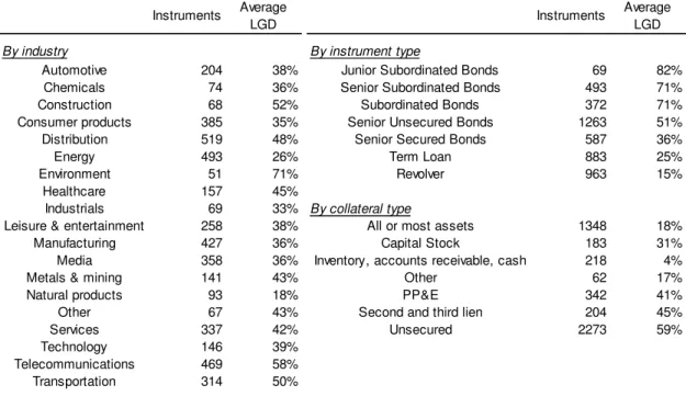
Table 2 reports the number of default instruments and average LGD by

industry, instrument type and collateral type. Industry representation across

default events included in the URD shows that the highest historical LGD is

found on Environment industry while the lowest is observed in the Natural

Products industry. Distribution, Energy, Telecommunications and Manufacturing

are the industries that provide more cases to the database, jointly representing

more than 40 percent of total defaulted instruments. Looking at the instrument

type breakdown we can see the importance of the priority-position of an

instrument within the obligor’s liability structure, since LGD vary significantly by

this factor. Average LGD ranges from 82 percent (Junior Subordinated Bonds)

to 15 percent (revolver loans).

Year Instruments Obligors Average

LGD Year Instruments Obligors

Average LGD

1987 23 4 24% 1999 184 54 43%

1988 64 9 45% 2000 271 67 49%

1989 98 21 54% 2001 572 98 48%

1990 150 28 52% 2002 783 112 51%

1991 226 51 42% 2003 399 77 30%

1992 190 38 39% 2004 206 47 27%

1993 138 32 38% 2005 203 29 24%

1994 66 23 31% 2006 75 18 28%

1995 96 28 34% 2007 47 12 25%

1996 83 24 36% 2008 197 43 34%

1997 64 18 35% 2009 370 82 37%

(31)

Page 31

Table 2 – Number of instruments and average LGD by industry, instrument type and collateral type. For recoveries rates greater than 100% it was considered a 0% LGD.

The breakdown by collateral type shows that debt secured by inventory,

accounts receivable and cash exhibit the lowest LGD. On the other side,

unsecured debt instruments have the highest historical LGD.

6. k-NN algorithm for LGD forecasting

Obtaining good results from k-NN algorithm depends crucially on the

appropriate feature and instance selection, distance / dissimilarity metrics,

neighborhood dimension (k) and local models. It is also important to conduct

model evaluation with proper performance metrics. Although all this tasks can

be embedded in the algorithm, that does not exempt model results from expert

critical analysis. The following sections show the several steps for developing a

k-NN algorithm for LGD forecasting, and testing its predictive accuracy against

historical averages and a more conventional parametric model. Instruments Average

LGD Instruments

Average LGD

By industry By instrument type

Automotive 204 38% Junior Subordinated Bonds 69 82%

Chemicals 74 36% Senior Subordinated Bonds 493 71%

Construction 68 52% Subordinated Bonds 372 71%

Consumer products 385 35% Senior Unsecured Bonds 1263 51%

Distribution 519 48% Senior Secured Bonds 587 36%

Energy 493 26% Term Loan 883 25%

Environment 51 71% Revolver 963 15%

Healthcare 157 45%

Industrials 69 33% By collateral type

Leisure & entertainment 258 38% All or most assets 1348 18%

Manufacturing 427 36% Capital Stock 183 31%

Media 358 36% Inventory, accounts receivable, cash 218 4%

Metals & mining 141 43% Other 62 17%

Natural products 93 18% PP&E 342 41%

Other 67 43% Second and third lien 204 45%

Services 337 42% Unsecured 2273 59%

Technology 146 39%

Telecommunications 469 58%

(32)

Page 32

6.1 Training and test data

Best practices in forecasting suggest that the predictive accuracy of a model

should be evaluated using out-of-sample data. Each training instance should

not be included in the test sample since it could lead to an artificial

overestimation of the model ability to forecast. For the same reason, out-of-time

data sample is also known as a good practice and should be considered as

well. In LGD forecasting the latter condition is even more compelling since there

is evidence of systematic risk in LGD (Hu & Perraudin, 2002; Altman et al.,

2005; Bruche & González-Aguado, 2010 and Acharya et al., 2007). Since LGD

is the result of a stochastic process, from default to emergence, and not a time

event, like default, it is also wise to consider a “pure” out-of-time sample, where

every instance from the test sample postdates all instances from training

sample. The effect of satisfying this condition has the drawback of excluding

from training sample recent LGD experience. We should expect that

out-of-sample and out-of-time test out-of-samples should perform “worst” than other out-of-samples

as they are not susceptible to over-fitting. This kind of evaluation truly replicates

model use in practice, and gives more reliable benchmark performance

indicators for generalization capacity and on-going model validation. For the

objective of this study, it was considered an almost fifty-fifty split between

training and test sample: defaulted instruments from 1987 to 2001 belong to the

training sample (2293 observations), and those from 2002 to the end of the

(33)

Page 33

6.2 Dimension reduction

6.2.1 Feature selection (and transformation)

Besides the abovementioned industry, instrument type and collateral type,

Moody’s URD comprises other variables that could be tested as determinants of

LGD. A filter approach based on expert judgement was performed in order to

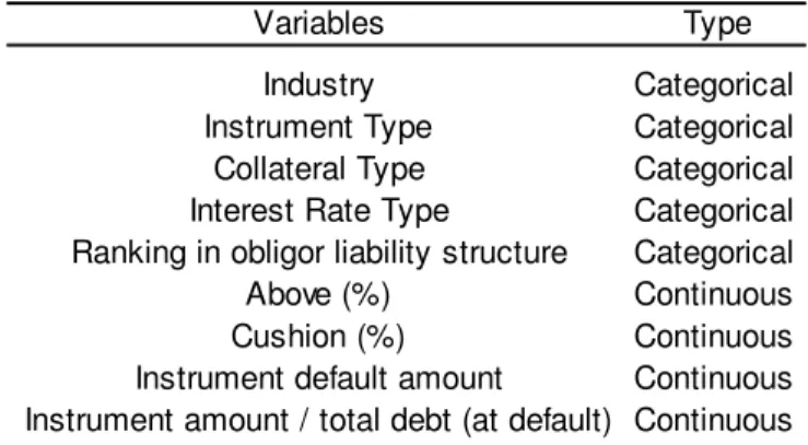
define the following initial set of explanatory variables:

Table 3 – Initial set of explanatory variables

Besides categorical variables mentioned in Table 2, Moody’s URD also includes

the Interest Rate Type of each credit instrument (fixed or variable, with different

indexes in the latter case) and the Ranking in obligor liability structure (ranging

from 1 – most senior – to 7 – most junior). Continuous variables include the

percentage of obligors’ debt senior to the defaulted instrument (Above %) and

debt outstanding junior to the defaulted instrument (Cushion %). It is also

considered as explanatory variable the instrument outstanding amount at

default and each instrument relative weight in obligors’ total debt at default.

From the initial set, categorical variables are individually evaluated before their

inclusion in the model. The performance of each of these features is

benchmarked against the use of historical average (see Appendix A). Features

that show better predictive power than the benchmark are included in the k-NN

algorithm. Based on the analysis carried out, all categorical features were

Variables Type

(34)

Page 34

selected for the k-NN algorithm. Selected categorical features have a “Forced

Entry” in the model, as the application of dissimilarity measures only to the

subset of these features often result in a number of ties greater than k, the

neighborhood dimension. In order to enable the usage of Goodall, IOF and OF

dissimilarity measures, categorical variables were then transformed and their

values were replaced by their correspondent frequency in the training sample.

For continuous variables two distinct approaches were tested: forced entry of all

subset (forming, with the subset of categorical variables, the “full model”) or

selection through the use of a wrapper method (forward selection). After the

forward selection, debt cushion and instrument amount / total debt at default

were added to the model from here on called the “forward model” (see

Appendix B).

Both Z-score transformation and min-max normalization were performed in

order to choose the one that maximizes model performance. Experiences

carried out showed better performance of the Z-score transformation. The

results presented in this paper consider this transformation for continuous

variables.

6.2.2 Instance selection

Using an out-of-time and out-of-sample test sample prevents the existence of

default instruments for the same obligor in both training and test samples. This

scenario could easily had lead to overfitting, since instruments for the same

query instance obligor could likely be in the k-nearest neighbors (distances

between instruments from the same obligor tend to be very short since they

(35)

Page 35

bigger for small k values and for local models that give greater importance to

closer neighbors, as these noisy instances would be overweighted. For the

same reason, it is worth to consider another reduction of redundant instances:

preventing each query neighborhood to have more than one instance (neighbor)

from the same obligor. After experiments carried out it was decided to allow

only one instance from the same obligor (the closest one) to be part of each

query instance neighborhood. Note that this is not a permanent deletion from

the training data, just a condition to be met on a query basis.

6.3 Distance / dissimilarity measures

Every distance / dissimilarity measure described in Section 3.4 was tested in

this study. For continuous variables, Euclidean distance proved to be the most

appropriate. The real challenge in this area is to find a proper dissimilarity

measure to deal with categorical variables. Each dissimilarity measure

mentioned above was tested for categorical features and combined with

Euclidean distance for continuous features as follows:

#

•*pq•* 3 `

!

>

•‘ ’

‘pq 3 `

1 (24)

where _“ and

K

are the number of categorical and continuous features,

respectively.

6.4 Neighborhood dimension and local models

In the tested models, neighborhood dimension was increased in multiples of 5

neighbors. The stopping criteria was met when the improvement in forecasting

performance indicators (see Section 3.7) was negligible. Once defined the

neighborhood, local models were applied. Due the nature of dataset features

(36)

Page 36

categorical and continuous features partial distances are combined, distances

between each neighbor and the query instance tend to be insensitive (i.e. to

change little) to weighted / kernel regressions mentioned in Section 3.6. Two

local models are tested in this study: the unweighted average presented in (16)

and a new weighted local model based on the distance between every k-1

neighbor and the closest (1-NN) neighbor. In the latter local model, the weight

U of each neighbor is given by the inverse of the min-max normalization of its

distance:

U k •* 3 ` +2 • 3 `

203 • 3 ` + 456 • 3 ` > m +

(25)

where ₇ _# and ₇₈ _# are the distances from query instance to

the closest and the furthermost neighbor, respectively. With this local model,

each neighbor weight (_U lies between 0.5 and 1.

Appendix C helps us understand which combination between distance /

dissimilarity measures and local model is better. Results show that the k-NN

algorithm performs better with the combination of IOF / Euclidean distances.

There is no significant difference between unweighted and weighted local

models for this distance combination. Best results are achieved at k = 35.

6.5 Results

The k-NN algorithm was applied to Moody’s URD and the results obtained were

compared to a fractional response model (see Appendix D) and to the use of

historical LGD averages. Two different k-NN models were fitted to the data: the

“full model”, with all features considered in the study (presented above in Table

3) and the “forward model”, with all categorical features and two continuous

(37)

Page 37

Both models were initially applied to the complete dataset, and then applied

separately to the subsample of bonds and the subsample of loans (see

Appendix E). Despite the existence of a small gain in predictive accuracy after

the forward selection of continuous variables, k-NN algorithm is apparently less

sensitive to the set of explanatory variables considered. k-NN forecasts clearly

dominate the forecasts given by the fractional response model and that

superiority in the full model is overwhelming when we weight errors by

instrument default amount. Considering all data, results in Table 4 show that

after some neighborhood growth (with optimal k between 35 and 40), k-NN

outperforms the benchmark parametric model and the historical average across

all measures, both in full and forward model. The root mean squared error in the

k-NN forward model is lower (0.325) than in the fractional response model

(0.339). When measuring the performance with wMAE and wRMSE it is

observable, in the full model, that the fractional response model has worse

predictive power than the historical average. However, in the forward model,

that situation no longer happens, which might indicate that the LGD forecasts

from the parametric full model are affected by the inclusion of the percentage of

debt senior to the instrument (Above %) and the instrument outstanding amount

at default. When considering the subsample of bonds, k-NN continues to

present better performance than the benchmark. Main conclusions about

models ability to forecast LGD dot not differ if we consider the entire data set or

if we consider bonds and loans separately. Nevertheless, is worth mentioning

that every model gives better predictions for loans than for bonds, perhaps due

to the difference in their LGD distribution (more concentrated and skewed to left

(38)

Page 38

(k=10) than in the subsample of bonds (k=40). This means that, when

comparing with bonds, we need less defaulted loans (i.e. less information) to

make a LGD estimate for a new defaulted loan.

Table 4 – Out-of sample and out-of-time predictive accuracy measures of LGD forecasts given by historical average, a fractional response model and a k-NN algorithm. Results presented refer to the entire data set and to the subsample of bonds and loans only.

7. Conclusion

This work shows that the nearest neighbor algorithm is a valid alternative to

more conventional parametric models in LGD forecasting. Using data from the

Moody’s Ultimate Recovery Database, it is shown that the k-NN algorithm tend

to outperformsthe factional response model, whether we consider the entire

All data

Full model Forward model

Fractional

response K-NN

Fractional

response K-NN

Mean absolute error 0.353 0.271 0.258 0.261 0.256

Root mean squared error 0.385 0.354 0.327 0.339 0.325

Relative absolute error (%) 100.00 76.99 73.25 73.93 72.50

Root relative squared error (%) 100.00 92.09 85.10 88.22 84.57

Weigthed mean absolute error 0.340 0.376 0.304 0.276 0.268

Weighted root mean squared error 0.374 0.478 0.356 0.350 0.335

Bonds

Fractional

response K-NN

Fractional

response K-NN

Loans

Fractional

response K-NN

Fractional

response K-NN

(39)

Page 39

data set or subsamples containing only bonds or loans. Unlike other machine

learning techniques, k-NN seems to be very intuitive. Each LGD estimate can

be easily detailed and reproduced. On the other hand, k-NN is very sensible to

the data itself. When using this algorithm to LGD forecasting, it is very important

to perform an adequate data dimension reduction (both in explanatory variables

and instances). Expert analysis is a major requirement if banks consider the use

of k-NN in LGD forecasting. Furthermore, this algorithm does not enable risk

analysts to know the marginal effect on recoveries of each variable and to

understand which variables are contributing to the forecasts.

It has been demonstrated that the nearest neighbor algorithm has potential to

be used by banks in LGD forecasting. From a deeper study of

distance/dissimilarity measures and weighted local models can surely result

better algorithms than the one presented in this work. This machine learning

technique has also potential to deal with other important (and sometimes tricky)

issues regarding LGD forecasting: deriving a downturn LGD (for example, by

considering only data from the recession period of the economic cycle in the

training set), the inclusion of unfinished recovery workouts (for instance,

combining NN with survival analysis) and LGD stress testing (i.e. including

(40)

Page 40 References

Altman, E., Brady, B., Resti, A. and Sironi, A. (2005). The link between default

and recovery rates: Theory, empirical evidences, and implications. Journal of

Business 78(6), 2203–2227.

Altman, E. and Kishore, V. (1996). Almost Everything You Wanted to Know

about Recoveries on Defaulted Bonds. Financial Analysts Journal, Vol. 52,

No. 6, pp. 57-64

Araten, M., Jacobs M., and Varshney, P. (2004). Measuring LGD on

commercial loans: An 18-year internal study. The RMA journal, 4:96–103.

Acharya, V., Bharath, S. and Srinivasan, S. (2007). Does industry-wide distress

affect defaulted loans? Evidence from creditor recoveries. Journal of

Financial Economics, 85:787–821.

Asarnow, E. and Edwards, D. (1995). Measuring Loss on Defaulted Bank

Loans: A 24 year study. Journal of Commercial Lending, 77(7):11-23.

Atkeson, C. and Schaal, S. (1995). Memory-based neural networks for robot

learning. Neurocomputing, 9, 243-269.

Atkeson, C., Moore, A. and Schaal, S. (1997). Locally Weighted Learning for

Control. Artificial Intelligence Review, 11, 11-73.

Bastos, J. (2010a). Forecasting bank loans loss-given-default. Journal of

Banking and Finance, 34, 2510–2517.

Bastos, J. (2010b). Predicting bank loan recovery rates with neural networks.

(41)

Page 41

Bellotti, T. and Crook, J. (2012). Loss given default models incorporating

macroeconomic variables for credit cards. International Journal of

Forecasting, Volume 28, Issue 1, Pages 171-182.

Bruche, M. and González-Aguado, C. (2010). Recovery rates, default

probabilities, and the credit cycle. Journal of Banking & Finance, Volume 34,

Issue 4, Pages 754-764.

Boriah, S., Chandola, V. and Kumar, V. (2007). Similarity Measures for

Categorical Data: A Comparative Evaluation. In Proceedings of the eighth

SIAM International Conference on Data Mining, 243-254.

Carey, M. (1998). Credit Risk in Private Debt Portfolios. Journal of Finance,

53(4):1363–1387.

Carty, L. and Lieberman, D. (1996). Defaulted Bank Loan Recoveries. Global

Credit Research, Moody’s.

Caselli, S., Gatti, S. and Querci, F., (2008). The sensitivity of the loss given

default rate to systematic risk: New empirical evidence on bank loans.

Journal of Financial Services Research, 34, 1-34.

Cunningham, P. and Delany, S. (2007). k-Nearest Neighbor Classifiers.

Technical Report UCD-CSI-2007-4, School of Computer Science and

Informatics, University College Dublin.

Davydenko, S. and Franks, J. (2008). Do Bankruptcy Codes Matter? A Study of

Defaults in France, Germany, and the U.K. The Journal of Finance,

63: 565–608.

Dermine, J. and Neto de Carvalho, C. (2006). Bank loan losses-given-default: A

(42)

Page 42

Felsovalyi, A. and Hurt, L. (1998). Measuring loss on Latin American defaulted

bank loans: A 27-year study of 27 countries. Journal of Lending and Credit

Risk Management, 80, 41-46.

Franks, J., de Servigny, A. and Davydenko, S. (2004). A comparative analysis

of the recovery process and recovery rates for private companies in the UK,

France, and Germany. Standard and Poor‘s Risk Solutions.

Frye, J. (2000). Depressing recoveries. Risk Magazine, 13(11):108–111.

Giese, G. (2006). A saddle for complex credit portfolio models. Risk 19(7), 84–

89.

Goodall, D. (1966). A new similarity index based on probability. Biometrics,

22(4):882-907.

Gourieroux, C., Monfort, A. and Trognon, A. (1984). Pseudo-maximum

likelihood methods: theory. Econometrica, 52 : 681-700.

Gower, J. (1971). A General Coefficient of Similarity and Some of Its Properties.

Biometrics, Vol.27, No. 4, 857-871.

Grossman, R., O’Shea, S. and Bonelli, S. (2001). Bank Loan and Bond

Recovery Study: 1997-2000. Fitch Loan Products Special Report, March.

Gupton, G., Gates, D. and Carty, L. (2000). Bank Loan Loss Given Default.

Global Credit Research, Moody's.

Gupton, G. and Stein, R. (2005). LossCalc V2: Dynamic Prediction of LGD.

Moody’s KMV.

Gürtler, M. and Hibbeln, M. (2011). Pitfalls in Modeling Loss Given Default of

Bank Loans. Working paper Series - Institut für Finanzwirtschaft, Technische

(43)

Page 43

Hu, Y. and Perraudin, W. (2002). The dependence of recovery rates and

defaults. Working paper, Birkbeck College.

Kullback, S. and Leibler, R. (1951). On information and sufficiency. The Annals

of Mathematical Statistics, Vol. 22, No. 1, 79-86.

Mahalanobis, P. (1936). On the generalised distance in statistics. Proceedings

of the National Institute of Sciences of India, Vol. 2, No. 1, 49-55.

Nadaraya, E. (1964). On estimating regression. Theory of Probability and Its

Applications, Vol. 9, 141–142.

Papke, L. and Wooldridge, J. (1996). Econometric methods for fractional

response variables with an application to 401(k) plan participation rates.

Journal of Applied Econometrics 11 : 619-632.

Scott, D. (1992). Multivariate Density Estimation. Wiley, New York, NY.

Shepard, D. (1968). A two-dimensional function for irregularly spaced data. In

23rd ACM National Conference, pp. 517–524.

Watson, G. (1964). Smooth Regression Analysis. The Indian Journal of

(44)

Page 44 Appendix A

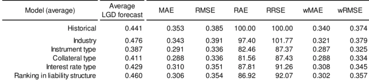
Table presents accuracy measures from simple models where LGD estimates correspond to the historical LGD average by each categorical variable value. Based on these results it was decided to include all the variables in the model.

Predictive accuracy measures

Model (average) Average

LGD forecast MAE RMSE RAE RRSE wMAE wRMSE

Historical 0.441 0.353 0.385 100.00 100.00 0.340 0.374

Industry 0.476 0.343 0.391 97.40 101.77 0.321 0.379

Instrument type 0.387 0.291 0.336 82.46 87.37 0.287 0.325

Collateral type 0.411 0.288 0.336 81.56 87.43 0.288 0.334

Interest rate type 0.429 0.310 0.351 87.81 91.26 0.308 0.345

(45)

Page 45 Appendix B

In this appendix are presented the results of the forward selection technique described in Section 3.5. In each step, (positive) negative values represent a (loss) gain in the predictive accuracy from the previous step. Categorical variables had a forced entry in the model and then, in step 1, the instrument amount / total debt at default entered the model. Later, in Step 2, cushion (%) joined the model. Larger improvement in accuracy measures was the criteria to select features each step (feature selection stopped in Step 3).

Forward model - feature selection

Distance/Dissimilarity measures: IOF + Euclidean distance Local model: weighted

k = 10

Change in predictive accuracy measures RMSE MAE RRSE RAE wRMSE wMAE Historical average - - -

-Forced entry:

Industry Instrument type Collateral type Interest rate type

Ranking in liability structure

Forward selection:

Step 1:

Instrument amount / total debt (at default) -0.006 -0.002 -0.016 -0.004 -0.007 0.0011

Step 2:

Cushion (%) -0.001 -0.014 -0.004 -0.039 0.0102 -0.005