Characterization of PET image using global and local entropy

(1)

BJRS

OF

RADIATION SCENCES

03-1A (2015) 01-16

Characterization of pet image using global and local

entropy

I.F. Vieira

1,2,5

; M. Koole

2

; J. W. Vieira

3,4

; F. R.A. Lima

1,5

1 _{Departamento de Energia Nuclear, DEN-UFPE} CEP 50740-540, Av. Prof. Luís Freire, 1000, Recife, PE

ifv.kul@gmail.com igor.vieira@student.kuleuven.be

2 _{Division of Nuclear Medicine, University Hospital Gasthuisberg,} K.U.Leuven. Herestraat 49, 3000, Leuven, Belgium.

michel.koole@uzleuven.be

3 _{Instituto Federal de Educação, Ciência e Tecnologia de Pernambuco,} IFPE Campus Recife, CEP 50740-540, Av. Prof. Luís Freire, 500, Recife, PE

4 _{Escola Politécnica de Pernambuco, EPP-UPE} CEP 50750-470, Rua Benfica, 455, Recife, PE

jose.wilson@recife.ifpe.edu.br

5 _{Centro Regional de Ciências Nucleares do Nordeste, CRCN-NE/CNEN} CEP 50740-540, Av. Professor Luiz Freire, 200, Recife, PE

falima@cnen.gov.br

ABSTRACT

In the clinical practice PET imaging provides semi-quantitative information about metabolic activities in human body, using the Standardized Uptake Value (SUV). The SUV scale, by itself, does not to establish thresholds between benign and malignant uptake in high-level analyses, such as pattern recognition. The objective of this work is to investigate in PET image volume with high-uptake regions, two additional descriptors, besides the SUV measurements: the amount of information given by the Hartley function (IHartley) and its expected value, the Shannon entropy (H). To estimate these

descriptors, two models of the probability distribution were obtained from a high-uptake region of interest (ROI): (i) the normalized grayscale histogram from SUV intensity levels (Pi), which provides

(2)

International Joint Conference RADIO 2014

(Pg,k) at the same range, which provides local IHL and HL. The beginning results have shown that for the

ROI (12x12 pixels) and for mean SUV ranging of 6.6213±0. 5196 g/ml, with SUVMax = 14,7372 g/ml, the global entropy (2,3778±0,0364) has a higher average uncertainty that local entropy (2,2069±0,0758), with a confidence interval of 99.95% (pvalue < 0,05%). This can be explained by analysing the sample from the amount of information, IHartley, noting that on average local Pg,k provides up to 90,55±9,18%

more information when compared to the amount of information given by global Pi. Therefore, these

initial results suggest that, for build algorithms for PET image segmentations using threshold based in entropy measures, it is more appropriate to use a distribution functions estimator which considers the local information of the pixels intensities. The main application of this approach will be for, among other things, to construct pathological phantoms from PET images for dosimetry applications.

Keywords:

Palavras-chave: colocar 3 palavras-chave (padrão DeCS).

1. INTRODUCTION

The Positron Emission Tomography (PET) is a method used to visualize physiological processes in living individuals, in the non-invasive way. The PET image is applied to early cancer diagnosis as well planning and monitoring complex treatments such as radiotherapy or chemotherapy [1, 2].

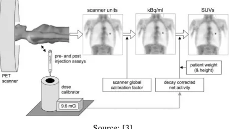
The functional changes are showed in the uptake of radiotracer injected into patient (example, 18F-FDG, a radioactive glucose anolog). The main indice used in clinical practice for measure it is the Standardized Uptake Value (SUV) [3] (Figure 1). It is important to emphasize that the SUV indice is linearly related to a set of random variables such as the image intensity, specific parameters of patient and scanner, as well the kinetics of tracer [2].

Recent studies have sought to increase the characterization of the uptake pattern from radiotracer with goal of lesions analysis [4, 5, 6, 7]. Once PET image has modest spatial resolution [3] and the SUV scale, by itself, is not sufficient to establish thresholds between benign and malignant uptake in high-level analyses, such as pattern recognition, it is important to find other tools that provide more information about the heterogeneity uptake distribution within tumor regions.

Therefore, the objective of this work is to investigate two additional descriptors in PET image with high-uptake regions, besides the SUV measurements: the amount of information given by the Hartley function (IHartley) and its expected value, the Shannon entropy (H).

To estimate these descriptors, two models of the probability distribution were obtained from a high-uptake region of interest (ROI), using: (i) the normalized grayscale histogram from SUV intensity levels (Pi), which provides global IHartley and HG; and (ii) the normalized gray level co-occurrence matrix (GLCM) of these graylevels (Pg,k) at the same range, which provides local

(3)

Figure 1. Acquisitions steps and processes for image in SUV scale.

Source: [3].

This paper is organized as follows: the Section 2 provides the theoretical framework. In the Subsection 2.1 the concepts of entropy will be described, as well as the mathematical formalisms. Section 3 the methodology will be presented in detail. Subsection 3.1 to show how the two models of the probability distribution (Pi and Pg,k) were obtained from a high-uptake ROI. Subsection 3.2 shows how to use these PDFs to generate local and global entropy. The experimental results are presented in Section 4 and conclusions will be shown in Section 5.

2.

THEORETICAL FRAMEWORK

2.1. ENTROPY CONCEPTS IN PHYSICS AND INFORMATION THEORY

Applications of Information Theory in pattern recognition has become increasing, due to its ability to identify and classify relevant random variables that characterize a given system. Naturally, it is possible when each pixel, in the case of images, is assumed as results from a set of random experiments such as in PET imaging [2]. Thus, an important concept in this subjective is the entropy concept.

Originally, entropy is a term that comes from thermodynamic physics. As developed, in the first instance, by Clausius, it is a state function expressed by:

(4)

where dQ and T are the heat and temperature of system, respectively. As consequence, the algebraic sum of all entropy variations in an irreversible process is always positive or, in reversible process, zero; i.e., ∆ ≥ 0, which corresponds to second law of thermodynamics [8].

Subsequently, Ludwig Boltzmann suggests an alternative, but equivalent definition:

= ( ) (2)

being the Boltzmann constant, and , the number of microstates related to the

observed thermodynamic microstate, also known as thermodynamic probability. However, in the mid-twentieth century, Shannon proposes a measure to quantify the uncertainty in the context of information theory, which became known as the Shannon Entropy1_{[9]. The Shannon Entropy is a functional of the probability function, p(x), where}

x is a random variable from a discrete set X = {x1, …, xn}, given by:

( ) = − ( ) ( )

(3)

Usually, the base b of the logarithm is 2. In this case, the entropy, H(X), is measured in

bits. Else, if the base b of the logarithm is the neperian base H(X) is measured in nants.

The Shannon entropy can also be seen as a mathematical expectation2 [9]:

( ) = − ( ) = ( ) (4)

where the value:

( ) = − ( ) (5)

in Eq. 4, it can be interpreted as the amount of information that describes the random variable , also called the Hartley information [9,10]. Thus, the H(X) represents a measure of the uncertainty of the system, mathematically representing a weighted mean of the Hartley information and meets the following mathematical properties [9,10]:

(1) For any , ( ("_#), … , ("_%)), is a continuous and symmetric function of variables x1, …, xn;

(2) Zero probability events do not contribute to the entropy, that is ( ("_#), … , ("_%), &

) = ( ("#), … , ("%)).

(3) The entropy is maximized when the probability distribution (") is uniform (

(") = (/*), i.e, for all x, we have:

+ ("#), … , ("%), ≤ .(_{* , … ,}_*/.(

1_{Originally, Shannon called this amount of “missing information”. Von Neumann was the one}

who suggested to call it as entropy, given their mathematical properties.

2_{In probability theory, the expected value or the mathematical expectation of a random variable}

(5)

This is a consequence of Jensen’s inequality [9]:

( ) = 8 _{( )9 ≤}( . 8 (_{*9/ =} *.

(4) Entropy of a set is additive, i.e., is equal to the sum of entropy of each subsets. (5) Entropy is a state function: given the probability (") between the initial and fina

l states, the entropy is independent of the path taken to achieve these states.

It is possible to not that the entropy is not a function of the random variable , but it is function of the probability distribution associated with this random variable. That is, the entropy does not depend on individual values that takes, but depend of the probabilities associated with each them. For this reason, is interpreted such as a measure of the uncertainty of system.

3. MATERIAL AND METHODS

3.1

Obtaining the Probability Distribution (PD) from ROI

The main problem in Shannon entropy estimating is how to get the PD associated from the system under analysis. There are several possible methods, such as histogram method [13] and kernel density estimation (KDE) as well [15].

However, the process used in this work is restricted to obtaining the PD from: (i) the normalized histogram (0 ≤ :_;( ) ≤ 1) and (ii) the normalized (0 ≤ : _, ( ) ≤ 1) co-occurrence matrix.

Let =( , >) an image represented by a two-dimensional array with ? @ pixels, and containing A gray levels in the range &, A_Bá . The histogram is represented by a vector D with A elements.

Thus, each image has a single histogram, and when it is normalized, the histogram can be seen as a discrete probability distribution and represents the chance to find a certain gray level in the image set. Considering this, the PD, :_;( ), can be expressed as [13]:

:;( ) = *;_* = D(;)_?@ (8)

where *_;= D(;) represents the number of occurrences of gray levels ;, and * = ?@ is the total number of pixels in the image =( , >).

However, this method has the disadvantage of supposing the pixels as independent and to ignore the spatial information. Moreover, it has the drawback that may be possible different images, with the same interval ( &, A_Bá ), presenting the same histogram. To overcome this limitation, and incorporate some spatial dependency between closed pixels, the co-occurrence matrix [12] was used in this work.

(6)

The co-occurrence matrix, = EF G

A A, of an image =( , >), is an matrix (A A) that

describes the frequency of intensity transitions between adjacent pixels. In other words, the i,j-th element of the matrix gives the number of times that the gray level j succeeds the gray level i, given a specific direction.

Let R the i,j-th pixel in =( , >) and r one of the eigth neighboring pixels of R, i.e.,

H IJ= K(;, L − (), (;, L + (), (; + (, L), (; − (, L), (; − (, L), (; − (, L − ()_{(; − (, L + (), (; + (, L − (), (; + (, L + ()} N

The number of times that the level succeeds the level in = EF G

A A in one of the eigth directions, is given by:

F = ∑I P,H IJOIH (9)

where:

OIH= Q(,_&,;= FDR HS> RTR ;* I ;U S* ;* H ;U _FDRHV;UR

Considering here only the horizontal displacement to the right (Figure 2a), the co-occurrence matrix can be defined as:

F = ∑ ∑ O?;7( @L7( ;L (10)

With

O;L= Q(& UR =(;, L) = R =(;, L + () =_FDRHV;UR

Thus, the probability of the point pair (g,k) that satisfies the operator O_;L is: : , = _∑AW(F _F

,

(11)

The Figure 2 shows how to obtain the co-occurrence matrix. The dimensions of this matrix are proportional to the number of gray levels, regardless of image size.

To obtain the invariant GLCM, in other words, the co-occurrence matrix to each possible directions X = 45[, 90[, 135[, the average between each correspondent pixel in each direction was computed (Figure 2b).

Figure 2. How the matrix of co-occurrence is generated. (a) The image has 8 gray levels and the position operator is defined as a pixel immediately to the right (X = 0[). (b) Other offsets

that can be defined for the operator, for example (X = 45[, 90[, 135[) [12]. In this work, the invariant GLCM [0[, 45[, 90[, 135[] was obtained. It is equivalent to get the average of each

(7)

(a) (b)

3.2

Global and Contextual Entropy

Using the PD from histogram (Eq. 8) in equations 3 and 5, we have the Global Hartley information and Global Shannon entropy, given by:

_^( ) = :_; (12)

^ :; :;

(13)

Making the same procedure with Eq. 11, using now the normalized co-occurrence matrix, we have the local information and following expressions:

_A : _, (14)

A : , : ,

(8)

An algorithm using Python programming language was developed [16] to compute the probability distribution from a high-uptake ROI. The open-source library, PyDICOM, [17] was used in this algorithm to read the PET DICOM files. Each ROI has 12x12 pixels, from row 80 to 92, and from column 100 to 112 in thoracic images of patient with lung cancer.

Figure 3 summarizes the steps for obtaining global and local Hartley information as well global and contextual entropy.

Figure 3. Steps for obtaining global and local Hartley’s information, and in consequence, global and contextual Entropy.

4. RESULTS AND DISCUSION

Since the sample has n = 20 images, the confidence interval, _ `, a), for the mean (b) was obtained for each variable using Eq. 14, where it is assumed that the standard error of the sampling distribution of b come from the T-Student distribution with significance

(9)

_ `, a) = b ± Fa U

√* (14)

Table 1 shows the results obtained for each entropy model, maximum and average SUVs. The Figure 4 shows as well an overview of the entropy behaviour.

Considering these two treatments to entropy estimation, obtained under same conditions, featuring a total of 20 pairs of observations, the hypothesis T-test could be appropriate to compare the closed entropies values in each ROI.

Thus, hypotheses can be formulated initially as follows:

(a) Null hypothesis (h0): HG = HL, i.e., the entropies are equal;

(b) Alternative hypothesis (h1): HG > HL, i.e., the local entropy is smaller than global

entropy.

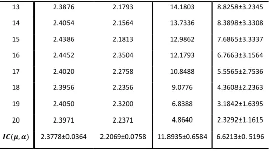
Table 1. Global and Local entropy in a ROI (12x12). Entropy

Legend Global Contextual SUVMax (ROI) SUVMean (ROI)

1 2.2812 2.0879 6.4358 2.7254±1.4592 2 2.3105 2.1028 9.1126 3.7182±2.1834 3 2.3124 2.1589 11.6338 4.7543±2.8990 4 2.3624 2.1097 13.6864 5.8585±3.5267 5 2.4037 2.1044 14.7372 6.8141±3.8544 6 2.4560 2.2692 14.6786 7.6628±3.8586 7 2.4499 2.1337 14.1113 8.3308±3.6353 8 2.3834 2.2367 13.5369 8.8254±3.3547 9 2.2993 2.1976 13.3577 9.1146±3.1670 10 2.3006 2.2571 13.5002 9.2251±3.0885 11 2.3541 2.3078 14.1086 9.2100±3.0840 12 2.3659 2.2365 14.2625 9.0872±3.1343

(10)

International Joint Conference RADIO 2014 13 2.3876 2.1793 14.1803 8.8258±3.2345 14 2.4054 2.1564 13.7336 8.3898±3.3308 15 2.4386 2.1813 12.9862 7.6865±3.3337 16 2.4452 2.3504 12.1793 6.7663±3.1564 17 2.4020 2.2758 10.8488 5.5565±2.7536 18 2.3956 2.2356 9.0776 4.3608±2.2363 19 2.4050 2.3200 6.8388 3.1842±1.6395 20 2.3971 2.2371 4.8640 2.3292±1.1615 _ `, a 2.3778±0.0364 2.2069±0.0758 11.8935±0.6584 6.6213±0. 5196

(11)

To compare the difference between these two methods based on probabilities distributions (Pi and Pg,k), as well the hypotheses formulated initially, the data are

considered in pairs, and the variation in entropy is calculated such as in Eq. 15. Results for each ROI are shown in Table 2.

∆ ^− A (15)

In terms of the difference, ∆ , the hypotheses (a) and (b) can be rewritten as: (c) Null hypothesis (h0): ∆ = &, the entropies are equal;

(d) Alternative hypothesis (h1): ∆ > 0, i.e., the local entropy is smaller than global

entropy.

Thus, given the sample, the hypotheses test can be obtained by:

F = ∆hhhh. √*_U (16)

where * is the size of the sample pairs (Table 2), ∆hhhh and U are the average and standard

deviation of the differences between the entropies models, respectively. The standard deviation is given by:

U = i_{* − ( . j}( ∆ ;k− *. ∆hhhhk ;

l (17)

Tabela 2. Difference between Global e Local Entropy (Eq. 13) at each ROI (12x12 pixels).

Legend _^ _S _{A mS} ∆ 1 2,2812 2,0879 0,1933 2 2,3105 2,1028 0,2077 3 2,3124 2,1589 0,1535 4 2,3624 2,1097 0,2527 5 2,4037 2,1044 0,2993 6 2,4560 2,2692 0,1868 7 2,4499 2,1337 0,3162

(12)

International Joint Conference RADIO 2014 8 2,3834 2,2367 0,1467 9 2,2993 2,1976 0,1017 10 2,3006 2,2571 0,0435 11 2,3541 2,3078 0,0463 12 2,3659 2,2365 0,1295 13 2,3876 2,1793 0,2084 14 2,4054 2,1564 0,2490 15 2,4386 2,1813 0,2573 16 2,4452 2,3504 0,0948 17 2,4020 2,2758 0,1262 18 2,3956 2,2356 0,1601 19 2,4050 2,3200 0,0850 20 2,3971 2,2371 0,1600 Mean 2,3778±0,0364 2,2069±0,0758 0.1709±0.0761

Using the equations 16 and 17, and Table 2, the threshold in T-test (F _nFRUF o. JJo) [17] is compared with:

F = ∆hhhh. √*_U = &. (p&q. √k&_{&. &pr( = (&. &oqJ}

Being F > F _nFRUF, with degrees of freedom ( = * – ( = (q), the test rejects the null hypothesis (h0) (∆ = &), in favor of the alternative hypothesis (h1): ∆ > 0, with significance level of 99.95% ( = &, &t%).

(13)

This result in T-test can be explained by analysing the sample from the amount of Hartley’s information, IHartley (Fig. 5). In average, the local distribution Pg,k, generated

from normalized invariant co-occurrence matrix (red plot), provides up to 90,55±9,18% more information when compared to the amount of information given by global distribution, Pi (blue plot). It explains results such as shown recently in Orlhac et Al, 2014

[19], where local entropy computed from co-occurrence matrix performs better than global entropy computed from unidimensional histogram, as well in the results shown by [5,6,7].

5. CONCLUSIONS

The beginning results have shown for the ROI (12x12 pixels) with SUV range of 11,8935±0,6584g/ml, and SUVMax = 14,74 g/ml (ROI 5, Table 2), that global entropy

(2,3778±0,0364) has a higher average uncertainty that local entropy (2,2069±0,0758), with a confidence interval of 99,95% (pvalue < 0,05%). This can be explained by analysing

the sample from the amount of information, IHartley, where in average the local distribution

Pg,k provides up to 90,55±9,18% more information by pixel, when compared to the

amount of information given by global Pi.. In other words, the local entropy computed

from Pg,k potentially provides more diagnostic information about the system, in the

context analysed in this work, PET image, than global entropy.

Therefore, these initial results suggest that: for build algorithms for PET image segmentations using threshold based in entropy measures, it is more appropriate to use a distribution functions estimator which considers the local information of the pixels

(14)

intensities. Measurements with larger sample (n > 20 images) will be performed and tools will

be built using information theory approach looking for, among other things, construct pathological phantoms from PET images for dosimetry applications.

6. ACKNOWLEDGMENTS

The authors thanks to CNPq/Brazil and FACEPE/Brazil by financial support to this project.

REFERENCES

1. Journal

CATANA C., PROCISSI D., WU Y., JUDENHOFER MS., QI J.,PICHLER B.J., JACOBS R.E., CHERRY S.R., Simultaneous in vivo positron emission tomography and magnetic resonance imaging, 105(10):3705-10, 2008.

2. Book

ZAID H., Quantitative Analysis in Nuclear Medicine Imaging., 1st Edition, New York, Springer, 2006.

3. Journal

P. E. KINAHAN, J. W. FLETCHER, Positron emission tomography-computed tomography standardized uptake values in clinical practice and assessing response to therapy, Seminars in ultrasound, CT, and MR volume 31 (6) (1 December 2010) 496{505. doi:10.1053/j.sult.2010.10.001.

4. Journal

FINBARR O’S., SUPRATIK R., JANET E., A statistical measure of tissue heterogeneity with application to 3D PET sarcoma data, Biostatistics (2003), 4, 3, pp. 433-448.

5.

EL NAQA, I., P. GRIGSBY, A. APTE, E. KIDD, E. DONNELLY, D. KHULLAR, S. CHAUDHARI, D. YANG, M. SCHMITT, RICHARD LAFOREST, W. THORSTAD, AND J. O. DEASY, Exploring feature-based

(15)

approaches in PET images for predicting cancer treatment outcomes, Pattern Recognit. Jun 1, 2009; 42(6): 1162–1171.

6.

H. M., C. LE REST C., VAN BAARDWIJK A., L. P., E. A. PRADIER O, Impact of tumor size and tracer uptake heterogeneity in (18)F-FDG PET and CT non-small cell lung cancer tumor delineation., J. Nucl, 2011, 1690-7.

7.

TIXIER F., REST C.C., HATT M., ALBARGHACH N., PRADIER O., METGES J.P., CORCOS L., VISVIKIS D., Intratumor heterogeneity characterized by textural features on baseline 18FFDG PET images predicts response to concomitant radiochemotherapy in esophageal cancer., J. Nucl. Med., 2011.

8. Book

ZEMANSKY, M. Calor e Termodinâmica . 5. Ed.: Guanabara, Edição Brasileira, 1978.

9.

COVER, T.; THOMAS, J. Elements of Information Theory. 1. Ed.: Wiley–Interscience Publication, New York, 1991.

10.

AVERY, J. Information Theory and Evolution, 1. Ed.: Cingapura: World Scientific, 2003.

11.

COVER, T.; THOMAS, J. Elements of Information Theory. 1. Ed.: Wiley–Interscience Publication, New York, 1991.

12. Journal

JANSING, E.; ALBERT, T.; CHENOWETH, D. Two-dimensional entropic segmentation. Pattern Recognition Letters, v. 20, p. 329–336, 1999.

13. Book

GONZALEZ, R.C. AND WOODS, R.E.(2008). Digital Image Processing, PEARSON- Prentice Hall, Reading.

14. Journal

ROUSSON, M. AND CREMERS, D. Eﬃcient Kernel Density Estimation of Shape and Intensity Priors for Level Set Segmentation, G. Gerig (Ed.), Medical Image Comput. and Comp.-Ass. Interv. (MICCAI), Palm Springs, Oct. 2005. LNCS Vol. 3750, pp. 757–764.

(16)

15. Book

MCLACHLAN, G. AND PEEL, D. (2000). Finite Mixture Models Wiley, New York.

16.

MCKINNEY, W. (2012). Python for Data Analysis, O’Reilly Media.

17. Website

PyDICOM User Guide, https://code.google.com/p/pydicom/, accesses in May 2014.

18. Book

BARBETTA, P.A., REIS, M.M and BORNIA, A.C., Estatística para Cursos de Engenharia e Informática, 3th Edition, page 379, Atlas, 2010.

19. Journal

ORLHAC F, SOUSSAN M, MAISONOBE JA, GARCIA CA, VANDERLINDEN B, BUVAT I., Tumor texture analysis in 18F-FDG PET: relationships between texture parameters, histogram indices, standardized uptake values, metabolic volumes, and total lesion glycolysis, J Nucl Med. 2014 Mar;55(3):414-22. doi: 10.2967/jnumed.113.129858. Epub 2014 Feb.