Plane detection from monocular image sequences

PLANE DETECTION FROM MONOCULAR IMAGE SEQUENCES

DCA - UFRN Natal, RN, Brazil email: kelson@dca.ufrn.br

Helder de J. Araújo ISR - DEEC - UC Coimbra, Portugal email: helder@isr.uc.pt

Adelardo A. D. de Medeiros DCA - UFRN Natal, RN, Brazil email: adelardo@dca.ufrn.br

ABSTRACT

Planes are important geometric features and can be used in a wide range of applications. This work aims to illustrate a homography-based method to detect planes using the affine model. Using two image frames from a monocular se-quence, a set of match pairs of interest points is obtained using Harris corner detector combined with the Scale In-variant Feature Transform (SIFT) as local descriptor. A Delaunay triangulation is performed on the set of detected corners of the first image and we use a triangle to calculate an affine homography that represents a plane in the image. An algorithm was developed to cluster interest points be-longing to the same plane based on the reprojection error of the affine homography. Tests are performed in differ-ent sequences of indoor and outdoor images and results are shown.

KEY WORDS

Computer Vision, Plane Detection, Affine Homography

1

Introduction

Planes are important geometric features and can be used in a wide range of computer vision applications like vision based robot navigation [1] and camera calibration [2]. Pla-nar surfaces present within a scene can provide useful in-formation on the environment. A pair of images captured by a stereo rig or a single moving camera can be used to extract such information.

A wide range related to plane detection are found in the literature [3,4]. In [5], the normal vector to a plane is estimated by using only three corresponding points from stereo images. A method for detecting multiple planar re-gions using a progressive voting procedure from the solu-tion of a linear system exploiting the two-view geometry is presented in [6]. SIFT (Scale Invariant Feature Transform) features were used in [7] to obtain the estimates of the pla-nar homographies which represent the motion of the major planes in the scene. They track a combined Harris and SIFT features using the prediction by these homographies. The approach presented in [1] detects three-dimensional planar surfaces using 3D Hough transformation to extract plane segment candidates. Finally, a detailed review and perfor-mance comparisons of planar homography estimation tech-niques can be found in [8].

This work presents a homography-based method to

detect and cluster planes using the affine model. The affine model was chosen because of its simplicity and because it allows good results. Using two image frames from a monocular sequence, a set of matched pairs of points is re-quired in order to estimate all planar homographies. Each affine homography represents a planar surface present in the scene. A matching process is performed to obtain this set using a Harris corner detector combined with a local descriptor. We use SIFT as local descriptor. An algorithm was developed to cluster interest points belonging to the same plane. Tests are performed in different sequences of indoor and outdoor images. Results are illustrated showing the detected planes and validating the proposed method.

The paper is organized as follows. Section 2 presents some aspects related to planar homographies, highlighting the affine model. In Section 3, the proposed approach is formulated and in Section 4 the results are shown and dis-cussed. Finally, Section 5 summarizes this work and some references are presented.

2

Planar Homography

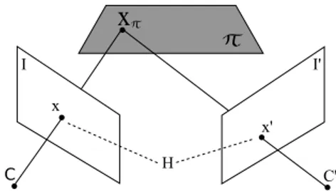
When a planar object is imaged from multiple viewpoints the images are related by a unique homography. Given two views of the same plane π = £

vT ₁¤T

, the ray corre-sponding to a pointxin the imageImeets the plane at a pointXπ, which projects intox’in imageI’. The map from x tox’ is the homography induced by the planeπ. This is shown in Figure 1. Therefore, the homography is deter-mined uniquely by the plane and vice versa [9].

Figure 1: Given a planar object imaged from two view-points, the planar homographyHis a mapping from points xof imageIto pointsx’of imageI’.

Given the projection matricesP = £

I|0¤T

andP’ =

£

plane is given by Equation 1.

x’=Hx, (1)

with

H=A−avT

In Equation 1xandx’are points in homogeneous co-ordinates. Therefore matrixHhas 9 entries, but is defined only up to scale, so the number of degrees of freedom in a 2D projective transformation is 8. Each corresponding 2D point generates two constraints on H by Equation 1 and hence the correspondence of four points is sufficient to computeH.

2.1 Affine homography

An affine homographyHAcan be defined as non-singular linear transformation followed by a translation. The matrix representation is formulated as in Equation 2

  x′ y′ 1  =  

a11 a12 tx

a21 a22 ty

0 0 1

 ·   x y 1   (2)

or in block form as in Equation 3

x’=HAx=

·

A t

0T 1

¸

·x. (3)

A planar affine homography has 6 degrees of freedom corresponding to the 6 matrix entries. Thus, the transfor-mation can be computed from three point correspondences, i. e., the homographyHAcan be computed from 3 matched pairs of points obtained using a pair of images captured by a stereo rig or a moving camera (monocular vision).

A modified version ofDirect Linear Transformation method is used to estimate the homography. The last row of an affine homographyHA is equal to£0 0 1¤, thus Equation 1 can be formulated in terms of an inhomoge-neous set of linear equations as Equation 4

       

x1 y1 1 0 0 0 0 0 0 x1 y1 1

x2 y2 1 0 0 0 0 0 0 x2 y2 1

x3 y3 1 0 0 0 0 0 0 x3 y3 1

        ·         h1 h2 h3 h4 h5 h6         =         x′ 1 y′ 1 x′ 2 y′ 2 x′ 3 y′ 3         , (4)

or in block form

X·HA=X’, (5)

wherexi =

£

xi yi¤

andx’i =

£

x′

i y′i

¤

are the matched pairs of points in inhomogeneous coordinates andHAhas the form of Equation 6

HA=





h1 h2 h3

h4 h5 h6

0 0 1



. (6)

To estimateHAfrom 3 matched pairs of pointsxi↔ x’i, i = 1,2,3, we can solve the Equation 5 using the pseudo-inverse as

HA= (XTX)−

1

·XTX’ (7)

whose computation is fast due to the low matrix dimen-sions.

2.2 Reprojection error

After an affine homographyHAhas been computed, an er-ror measure can be considered in order to verify whether a given matched pair of points belongs to the plane repre-sented byH_A. We use thereprojection errorwhich can be defined as

ei=|xi−ˆxi|

2

+|x’i−ˆx’i|

2

, (8)

whereˆx’i=HAxandˆxi=H−

1

A x’.

When the reprojection error ei is below a certain threshold, we consider that the given matched pairxi↔x’i belongs to the plane represented byHA.

3

Plane Detection

A plane detection method is presented in this section. Inter-est points are detected using the Harris corner detector [10] in two acquired images (stereo rig or monocular sequence), and a set of corresponding points between these images are created using a local descriptor like SIFT [11]. After this step the Delaunay triangulation is performed on the set of interest points of the first image. Using the set of triangles resulting from the Delaunay method, a filtering scheme is applied to discard degenerate triangles. From this new set of triangles and the set of matched pairs of points from the combined Harris detector and SIFT descriptor, we compute the homographies and perform a clustering scheme to de-tect planes present in the imaged scene.

The entire methodology used is described in the fol-lowing sections.

3.1 Interest points detection

Different primitives to detect and match image points ex-ist in the literature [12]. The Harris corner detector was chosen since it is fast, reliable and provides good repeata-bility under varying rotation and illumination. The Harris’ method is based on the computation of a matrix,M, using the partial derivatives of the intensity function

M =w⊗

   ³ ∂I ∂x

´2 ³

∂I ∂x

´

·³∂I ∂y ´ ³ ∂I ∂x ´

·³∂I_∂y´ ³∂I_∂y´ 2



 , (9)

A corner is detected thresholding a measure based on the determinant and trace of matrixM (equation 9).

M =

µ

A C C B

¶

det(M) =AB−C2

trace(M) =A+B

R=det(M)−k(trace(M))2

(10)

where k is constant and empirically adjustable, andR is called corner response. Points with R above a certain thresholdTh are considered a corner. In order to elimi-nate weak corners a non-maximal suppression procedure is performed in the neighborhood of a detected corner.

3.2 Local descriptor

Following the detection of interest points in two consecu-tive images, a local descriptor must be used to establish a measure of correlation between the possible candidates to a matched pair of corners. This work uses the Scale In-variant Feature Transform descriptor. The combination of Harris detector with the SIFT descriptor can be considered as a good choice because it produces good, fast and stable results [13].

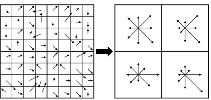
The SIFT descriptor is a local descriptor highly dis-tinctive and invariant to changes in illumination and 3D viewpoint. The descriptor is based on the gradient mag-nitude and orientation of all pixels in a region around the keypoint. These are weighted by a gaussian window and accumulated into orientation histograms summarizing the contents over subregions, as shown in Figure 2. The length of each arrow corresponds to the sum of the gradient mag-nitudes near that direction within the region.

Figure 2: This figure shows a2×2descriptor array com-puted from an8×8set of samples. Each descriptor has 8 bins. The descriptor is represented by a vector of size 32 (2×2×8).

The orientation histogram entries corresponding to the lengths of the arrows is in the bottom of Figure 2. The descriptor is formed by a vector containing all these entries. The distance between histograms (SIFT descriptor) is used as measure of correlation. A simple Euclidean mea-sure of distance is used. If the distance is below a certain threshold then a possible matched pair is detected.

3.3 Regressive corner filtering and matching

A regressive filtering scheme is used to establish a corre-spondence between the detected corners to find matched pairs.

For each detected corner in the first image, a corre-spondent corner is searched for in a neighborhood in the second image satisfying a correlation measure described in Section 3.2. All corners in the first image, which do not have a correspondent in the second image are discarded. In the next step, a regressive filtering is performed to prevent that two or more corners of the first image have the same match in the second image. Now, for every corner in the second image 2, only the best correlated corner in the first image is maintained. At the end of the filtering, a set of matched pairs of cornersM is obtained from the two im-ages.

GivenM, a Delaunay triangulation is performed only on the detected corners of the first image. Since the set of triangles has been obtained, a filtering scheme is applied to discard triangles that probably belong to virtual planes in the image. Only triangles with all sides within a cer-tain range of lengths are considered valid. Still triangles with valid sides can have their vertices almost collinear. Collinearity of the three points used in the computation of the affine homographies must be avoided. To solve this problem, triangles with areas less than a certain value are also discarded. An example of Delaunay triangulation and filtering scheme applied to an indoor image frame is shown in Figure 3.

(a) Delaunay triangulation (b) Result from triangle filtering

Figure 3: Example of Delaunay triangulation and triangle filtering performed in indoor images.

The next step consists on a clustering scheme. The new set of trianglesTobtained from the filtering scheme is used in a voting procedure to join points belonging to the same plane in the image. This is explained in the following section.

3.4 Clustering points

Given the set of matched pointsM and the set of fil-tered Delaunay trianglesT, we defineHpas the set of allp homographies existing between the two images. Each ho-mography inHpdefines a plane in the image. InitiallyHp is considered as empty. The first affine homography HA is computed using the three points of the first triangleT(1)

and their matched pairs in the setMaccording to the Equa-tion 7. HomographyHA thus obtained is included inHp, and all used points are marked as visitedand assigned to the homographyHp(1), i.e., the first plane.

In the next step, the next triangle of T and their matched points inM is considered. For eachHp(i)inHp, all points of the triangle are checked to determine whether they belong to any of the existing planes inHp. If the point had been marked asnot-visitedand the reprojection error forHiis below a certain threshold, the point is marked as visited and assigned to homographyHi. If the point had been marked asvisitedand if the new reprojection error for Hi is smaller than the previous one, the point is assigned to planeHi. In the case where all points of the triangle do not belong to any existing plane, a new affine homography HAis computed with those points. The new homography represents a new plane and is included inHp. This loop is performed until there are no unvisited matched pairs of points.

The clustering method described before can be de-scribed in the Algorithm 1.

At the end of clustering stage, only planes with a num-ber of points above a certain threshold are considered.

4

Experimental Results

In this section we report experiments that demonstrate ac-curate plane detection from two consecutive frames of an image sequence. Four image sequences of different out-door scenes were acquired by a camera. All used images in the experiments are in gray level with size640×480.

Different parameters were empirically adjusted at each stage of the entire process of plane detection. The following sections discuss each one of them.

4.1 Interest point detection

At this stage, the Harris detector was implemented using k = 0.13and a gaussian window with standard deviation σ = 1.5and size of6σ×6σ. A threshold valueTh was used to distinguish between corners and non-corners. Th must be set high enough to avoid the detection of false cor-ners which may have a relatively large corner responseR (Equation 10) due to noise. The value ofThis based on the maximum corner response computed, Rmax. It was used Th = 0.01·Rmax. After all corners had been detected, a non-maximum suppression scheme was performed with a window of size10×10, in order to eliminate weak corners.

Algorithm 1Clustering coplanar points. 1 Create an empty set of homographiesHp 2M: set of matched points between two images 4T: set of triangles of the first image

5t: number of triangles inT 6err: reprojection error

7Te: reprojection error threshold

TakeM andT(1), computeHAand put inHp

Assigned the three points of the triangleT(1)toHp(1), and mark them asvisited

forj = 2 :tdo

fori= each one inHpdo foreach pointpofT(j)do

ifp=not-visitedthen iferr<Tethen

AssignptoHp(i)

Markpasvisited end if

else ifp=visitedthen iferr<erroldthen UpdateptoHp(i)

end if end if end for end for

ifAllpofT(j)=not-visitedthen Compute newHAand put inHp

Assign allpto the newH_Aand mark them asvisited end if

end for

4.2 Local descriptor

The best results were obtained using SIFT with4×4 de-scriptors computed from a 16×16 sample array. The weighting gaussian window has size16×16andσ= 1.5. Each descriptor is described by an orientation histogram with 8 bins, each one of sizeπ/4. The total size of SIFT descriptor is 128 (4×4×8).

A simple Euclidean distancedwas used to compare descriptors. Ifd < Tmthen we have a possible matched pair of interest points. It was initializedTm= 10.

4.3 Regressive corner filtering and matching

In the regressive corner filtering and matching stage, we must perform a search in the second image for a corner that best matches a specific corner in the first image. This should be done for all detected corners in the first image. The size of the region of search can be constrained to im-prove the computational efficiency of the algorithm. This region can be defined based on the largest displacement of pixel, i.e., based on the camera’s movement during the ac-quisition process. In our case a region around the interest point of size25×25was used.

process of matching. When a possible match is found, the value of the threshold Tm is updated with the computed distanced. This was done to allow that the best candidate is chosen as a match.

As explained in Section 3.3, Delaunay triangulation is performed, followed by triangle filtering. Only triangles with sides of length between 5 and 80 pixels, and area over 10 pixels×pixels, are considered as valid.

4.4 Clustering points

Only one parameter is adjustable at this stage. A reprojec-tion error threshold was empirically chosen asTe = 3.0. The value ofTeis dynamically updated during the cluster-ing process. Thus, each matched pair of points in the set M is assigned to the best homography in the setHpbased on the computed reprojection error.

4.5 Results

Many different sequences were used in the experiments. Due to paper size restrictions only few results are shown here. Sequences with planes at different positions and ori-entations in the scene were chosen.

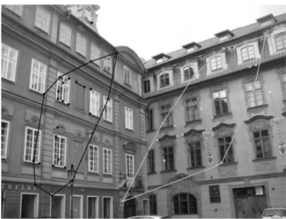
The planes detected are shown using geometric mark-ers in the first frame of each sequence. The results for out-door sequences are shown in Figures 4, 5 and 6.

Figure 4: Detected planar regions in outdoor sequence 1.

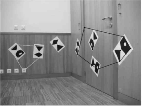
The results for indoor sequences are shown in Fig-ures 7, 8 and 9.

4.6 Discussion

The sequences were acquired under different conditions of illumination and different positions of the camera relative to the planes in the scene. The best results were obtained using Harris corner detector combined with SIFT descrip-tor in the matching process.

The matching process is one of the most important stages of the algorithm. An important parameter is the size of the region in which a match is searched for.

Figure 5: Detected planar regions in outdoor sequence 2.

Figure 6: Detected planar regions in outdoor sequence 3.

Each one of the image sequences used in the experi-ments presents two major planes of a scene. In some cases of indoor scenes, more than two planes were detected (Fig-ure 8. The results clearly show that the algorithm performs well using indoor and outdoor images.

5

Conclusion

In this paper we present a homography-based method for detecting planes. The affine model was chosen for its sim-plicity. In order to obtain a set of matched points between two frames of an image sequence, the Harris corner de-tector combined with SIFT descriptor and a regressive fil-tering method was used. Delaunay triangulation was per-formed on the set of corners of the first image frame. In order to avoid degenerate configurations in the estimation of the affine homographies, a triangle filtering scheme was used to discard triangles that would likely represent virtual planes.

Figure 7: Detected planar regions in indoor sequence 1.

Figure 8: Detected planar regions in indoor sequence 2.

Acknowledgements

This work is partially supported by the CAPES Foundation under grant no. 1087/07-0.

6

References

[1] K. Okada, S. Kagami, M. Inaba and H. Inoue, Plane segment finder: algorithm, implementation and applica-tions,Proc. IEEE Int. Conf. on Robotics and Automation, Seoul, Korea, 2001, 2120-2125.

[2] P. F. Sturm and S. J. Maybank, On plane-based camera calibration: A general algorithm, singularities, applica-tions,Computer Vision and Pattern Recognition,1, 1999, 432-437.

[3] D. Sinclair and A. Blake, Quantitative planar region detection, Int. Journal of Computer Vision,18(1), 1996, 77-91.

[4] Q. He, C-H. H. Chu, Planar surface detection in image pairs using homographic constraints, Proc of Int. Symp. on Visual Computing, Lake Tahoe, Nevada, USA, 2006, 19-27.

Figure 9: Detected planar regions in indoor sequence 3.

[5] J. Piazzi and D. Prattichizzo, Plane detection with stereo images,Proc. of IEEE Int. Conf. on Robotics and Automation, Orlando, Florida, USA, 2006, 922-927.

[6] G. Silveira, E. Malis and P. Rives, Real-time robust detection of planar regions in a pair of images,Proc. of Int. Conf. on Intelligent Robots and Systems, Beijing, China, 2006, 49-54.

[7] R. Rodrigo, Z. Chen and J. Samarabandu, Feature motion for monocular robot navigation,Proc. of Int. Conf. on Information and Automation, Colombo, Sri Lanka, 2006, 201-205.

[8] A. Agarwal, C. V. Jawahar and P. J. Narayanan, A survey of planar homography estimation techniques, Technical Report IIIT/TR/2005/12, Centre for Visual Information Technology, 2005.

[9] R. Hartley and A. Zisserman,Multiple view geometry in computer vision (Cambridge, UK: Cambridge University Press, 2004).

[10] C. Harris and M. Stephens, A combined corner and edge detection, Proc. of 4th Alvey Vision Conference, Manchester, UK, 1988, 147-152.

[11] D. Lowe, Distinctive image features from scale-invariant keypoints,Int. Journal of Computer Vision,20, 2003, 91-110.

[12] K. Mikolajczyk and C. Schmid, Scale and affine invariant interest point detectors,Int. Journal of Computer Vision,60(1), 2004, 63-86.