Coherent structures in open channel flows with bed load transport over an hydraulically rough bed

(1)

Bruno José Oliveira Santos

Licenciado em Ciências de Engenharia Civil

Coherent structures in open channel

flows with bed load transport over an

hydraulically rough bed

Dissertação para obtenção do Grau de Mestre em Engenharia Civil – Perfil de Estruturas

Presidente: Arguente: Vogais: Júri:

Professor Doutor Nuno Manuel da Costa Guerra Professor Doutor João Gouveia Aparício Bento Leal Professor Doutor Mário Jorge Rodrigues Pereira Franca Professor Doutor Rui Miguel Lage Ferreira

Dezembro 2013

Orientador:

Co-orientador:

Professor Doutor Mário Jorge Rodrigues Pereira da Franca,

Professor Auxiliar,

Faculdade de Ciências e Tecnologia,

Universidade Nova de Lisboa

Professor Doutor Rui Miguel Lage Ferreira,

Professor Auxiliar,

(2)



(3)

Coherent structures in open channel flows with bed load transport over an hydraulically

rough bed

(4)

(5)

O caos é uma ordem por decifrar.

(6)

(7)

À Quirina

(8)

(9)

Acknowledgements

O mérito não é estanque. É com esse pensamento que quero expressar a minha gratidão a todos quantos contribuiram para chegar aqui.

Quero começar por deixar o meu agradecimento ao orientador e co-orientador, respectiva-mente o Professor Mário Franca e o Professor Rui Ferreira.

Ao Professor Mário Franca agradeço a oportunidade e os ensinamentos, muitos transmitidos ainda antes de se pensar sequer que esta dissertação iria existir. Pela sua generosidade sempre presente, pelas suas indicações e principalmente por me apresentar esta incognita incrivel que é a hidráulica.

Ao Professor Rui Ferreira quero agradecer principalmente a sua confiança, disponibilidade em me acolher e por ter sido um guia essencial ao longo de todo o caminho. O seu rigor, método e sentido critico foram ferramentas imprescindiveis à conclusão desta dissertação.

Agradeço à Quirina por ser incansável no seu apoio, pela ajuda e motivação. Sem ti, nada disto seria possivel. És uma inspiração.

Aos meus pais José e Maria, eu devo tudo. Obrigado por acreditarem sempre, a vossa presença é inestimável.

O meu agradecimento vai também para toda a família, que esteve sempre presente na minha vida e foi parte integrante na minha formação pessoal. Entre todos destaco os meus irmãos Pedro e Helena, e incluo os mais novos, o André, o João e a Rita por serem sempre verdadeiros e me fazerem sorrir tantas vezes.

Não posso deixar de agradecer a amizade de todos aqueles que se têm cruzado no meu cami-nho. O Vitor pela pequena grande ajuda nas questões de programação, a Joana, o Ricardo, o Pedro e o António por serem sempre um grande apoio e por todos os bons momentos que passamos juntos. Ao Rodrigo, ao Sérgio e ao Jorge pelo companheirismo e pela amizade.

Agradeço também a todos aqueles que contribuiram para a minha formação. Ao longo do meu percurso académico cruzei-me com muitos professores em que cada um deu o seu contributo. É para eles que vai este meu agradecimento.

Deixo ainda o meu obrigado a todos os que de uma forma ou de outra têm contribuido para a formação de uma pessoa melhor.

(10)

(11)

Abstract

The degradation of forests through the impacts of devastating wildfires increase unprotected soils area which consequently favours soil erosion processes. The sediment production is continuously reaching water courses in these areas which may result in important impacts in the flow morphodynamics and hydrodynamics.

Sediment overfeeding induces important changes in the turbulent structure of the flow, mainly in momentum fluxes and exchange of momentum and mass between different layers in the flow structure, consequently affecting its ecological features.

Coherent structures play an important role on sediment transport and mixing processes which are important in the fluxes that govern the turbulent structure.

This study is aimed at evaluating the impacts of sediment transport on flow hydrodynamics, namely on the statistics characterizing coherent movements.

In order to accomplish the purposed objective, experimental tests were undertook in labora-torial environment where two-dimensional instantaneous flow velocity fields in both directions, streamwise and vertical, were measured through means of Particle Image Velocimetry (PIV) technique.

Two laboratory tests were simulated, consisting on a framework gravel bed with sand matrix and a framework gravel bed with sediment transport imposed at near capacity conditions. For both tests, the quadrant threshold analysis technique was employed and shear stress distribution statistics were analysed and discussed in what concerns their contribution and persistence.

The results show that, in the near bed region, mobile bed conditions make sweep events assume a major role in the shear stress production processes. Also, larger events become less frequent in the pythmenic region, comparing with the immobile bed results.

The impacts of mobile sediment in the near bed region over the flow structure are analysed and discussed in detail through probability density function distributions, in dimensional and non-dimensional data.

(12)

(13)

Resumo

A degradação da floresta através de fogos florestais aumenta a área de solos desprotegidos, o que consequentemente é favorável aos processos de erosão do solo. A produção de sedimentos atinge continuamente os cursos de água existentes nessas áreas, o que resulta num impacto importante sobre os processos morfodinâmicos e hidrodinâmicos do escoamento.

O excesso de sedimentos introduz alterações importantes na estrutura turbulenta do escoa-mento, principalmente nos fluxos de momento e troca de momento e massa entre camadas do escoamento, afectando as suas caracteristicas ecológicas.

As estruturas coerentes têm um papel importante no transporte de sedimentos e processos de mistura que se revelam importantes nos fluxos que controlam a estrutura turbulenta.

Este estudo foca-se na avaliação do impacto que o transporte de sedimentos tem na hidrodi-nâmica do escoamento, tal como nas estatisticas que caracterizam dos movimentos coerentes.

Visando atingir o objectivo proposto, foram efectuados ensaios em ambiente laboratorial, em que foram medidos campos bidimensionais de velocidade instantânea de escoamento nas direcções longitudinal e vertical, através da técnicaParticle Image Velocimetry(PIV).

Foram efectuadas duas experiências laboratoriais, uma sobre um leito composto por uma estrutura de seixo com uma matriz de areia e uma outra nas mesmas condições com excepção do facto de haver imposição de transporte de sedimentos. Para ambos os ensaios, foi aplicada a técnica de análise de quadrante e foram analisadas as estatisticas de distribuição da tensão de corte de Reynolds em que foi discutida a sua contribuição e persistencia.

Os resultados mostram que, na região junto ao leito, as condições de leito movél levam a que os eventos de varrimento assumam um papel preponderante na geração de tensão de corte de Reynolds. E também, que eventos de maior escala tornam-se menos frequentes na região pythménica, em comparação com os resultados do leito imóvel.

O impacto da existência de sedimentos móveis, na região junto ao leito, sobre a estrutura do escoamento são analisados em detalhe através de distribuição de função de densidade de probabilidade, para o caso de dados dimensionais e adimensionais.

(14)

(15)

List of Tables

2.1 Boundary layer regime and the correspondent Reynolds numbers (Re∗_{) that characterise it}

(Nezu and Nakagawa, 1993). . . 7

5.1 Main characteristics of experiments S3 and S4 (Amatruda, 2009). . . 34

5.2 Geometrical characteristics of the bed (Amatruda, 2009). . . 34

5.3 Mean flow characteristics of tests S3 and S4 (Amatruda, 2009).. . . 36

5.4 Non-dimensional parameters of experiments S3 and S4 (Amatruda, 2009). . . 37

5.5 Water temperature measured at the beginning and at the end of experiments S3 and S4 (Amatruda, 2009). . . 38

5.6 Some positioning and size characteristics of the acquired data . . . 39

6.1 Average and extreme values of the parameters calculated at reference point (1,4) in both mobile (S3) and immobile (S4) bed conditions. Where T represents the duration, A is the maximum shear stress, M is transported momentum and P is the period of events. . . 60

(18)

(19)

List of Figures

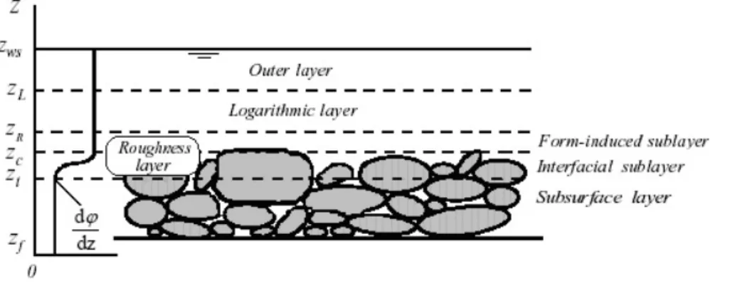
2.1 Layering system proposed by Nikora et al. (2001) for impermeable rough beds in open-channel flow conditions. Zstands for the distance to the bed,zcstands for the elevation

of highest roughness crests,Zf is the elevation of impermeable floor supporting particles,

ZLis the elevation of upper bound of logarithmic layer,ZRis the elevation of lower bound

of logarithmic layer,ztis the elevation of the deepest through,Zwsstands for free surface

elevation andϕis the void function. . . 8

2.2 Layering system proposed by Nikora et al. (2001) for permeable rough beds in open-channel flow conditions.. . . 8

2.3 Flow structure proposed by Ferreira et al. (2012) for permeable rough beds with sediment bed-load in open-channel conditions. hstands for the flow depth,Zbstands for the

boun-dary zero elevation,Zcstands for the highest crest elevation,Zsstands for the elevation of

the free-surface andZt is the elevation of the deepest through. . . 10

2.4 Top: Detail ofu′andw′. Bottom: Detail of_|u′w′_|(Ferreira et al., 2009). . . 12

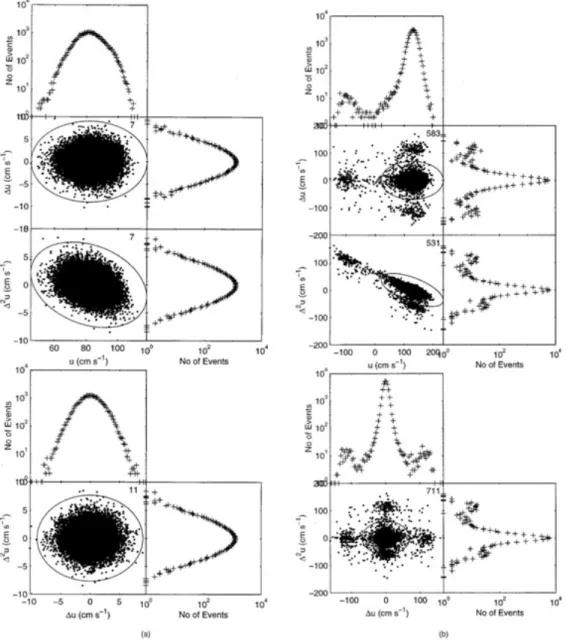
2.5 Example of a quadrant plot of the instantaneous flow velocity with thresholds. Obtained with bed load conditions in the overlapping between hyporeic and pythmenic regions and at the deepest position into the through. . . 13

3.1 PIV experimental setup. Adapted from Raffel et al. (1998). . . 16

3.2 Synchronization of the CCD camera with the laser pulses. From Lory (2011). . . 16

3.3 A pair of images in the same frame position, results in an average displacement in an interrogation area (Raffel et al., 1998). . . 17

3.4 Example of a correlation plot. The peak corresponds to the coordinates where the mean displacement estimation stands (Tropea et al., 2007). . . 18

3.5 Laser sheet thickness (Raffel et al., 1998). . . 19

3.6 Example of a peak-locking phenomena in the correlation plot. The true peak is wrapped between noise (Ferreira et al., 2010). . . 20

(20)

3.8 Light scattering resulting from a glass spherical particle in water, with a diameter

of 1µm. Adapted from Lory (2011). . . 23

3.9 Light scattering resulting from a glass spherical particle in water, with a diameter of 10µm. Adapted from Lory (2011). . . 23

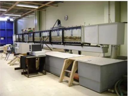
4.1 General view of the recirculating tilting flume at the Laboratory of Hydraulics and Envi-ronment of Instituto Superior Tecnico. . . 26

4.2 Support carriage that slides along the flume to help during measurements. . . 26

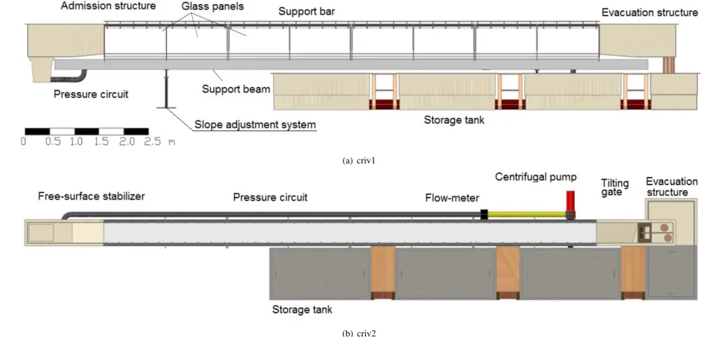
4.3 Schematics of the recirculating tilting flume and its main components. a) Plan view; b) Side view. Adapted from Ricardo (2008). . . 27

4.4 Slope adjustment structure composed by an electric motorized system. . . 28

4.5 Example of one of the four storage tanks. . . 28

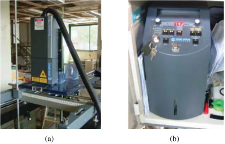
4.6 (a) Centrifugal pump used during the experiments. (b) Digital flow-meter used to measure the flow rate inserted in the flume. . . 29

4.7 (a) Downstream evacuation pipes. (b) Tilting gate used to adjust the free surface elevation. 29 4.8 A pair of laser safety glasses. . . 30

4.9 (a) A 0.5 mm precision ruler used to measure the free-surface elevation. (b) Digital ther-mometer. . . 30

4.10 Point gauge, with 0.1 mm, used to determine bed topography.. . . 30

4.11 (a) Laser head mounted on the support carriage. (b) Power supply used in the experiments. 31 4.12 CCD camera on a tripod. . . 31

4.13 Example of a laser light pulse. From Lory (2011). . . 32

5.1 Grain size distribution of the sand (left) and coarse-gravel (right) (Ferreira, 2008). . . 34

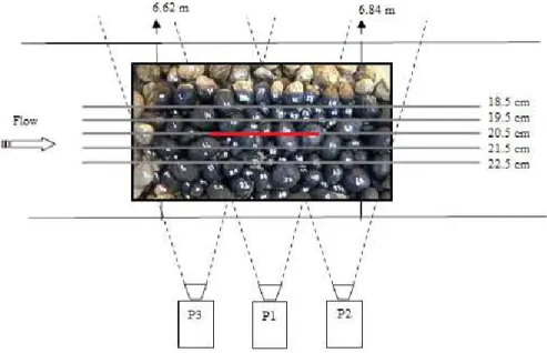
5.2 Measurement area, adapted from Ferreira (2008). . . 35

5.3 Extrapolation ofτ(₀2)from the total shear stress profile . . . 37

5.4 Camera position. Adapted from Ferreira (2008). . . 39

5.5 Calibration board used to set the longitudinal position of the camera (Ferreira, 2008). . . 39

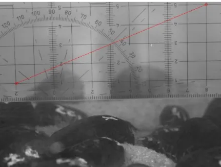
5.6 Example of a calibration image with a pair of points marked for calibration purposes. . . 41

5.7 Example of a mask used to neglect the bed roughness where it is known that any displa-cement in the data represents spurious data. The filtering mask in represented in red and fits the bed roughness.. . . 42

(21)

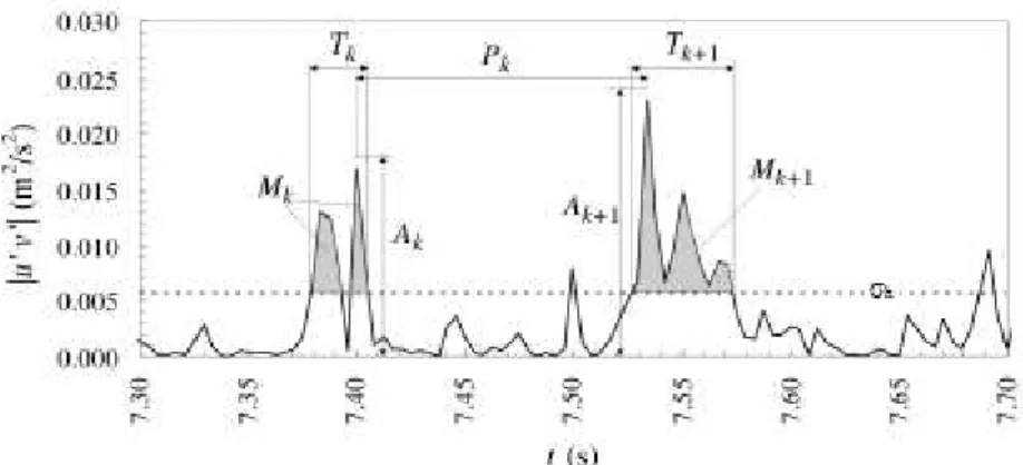
5.9 Definition of the parameters that characterize events in a u′w′ time series. The figure corresponds to the data in a unique reference position plotted against time. Adapted from

Ferreira et al. (2009). . . 48

5.10 Detailed event in a time series. The red segments have to be sliced because the event only starts over the threshold. Green segments are intermediate data.. . . 49

5.11 Quadrant plot of the initial segment of an event. P2 is in the sweep event area but the sweep event starts with the interception between the segment P1P3 and the thresholdσh. 49 5.12 Example of a sensitivity curve of the transported momentum to the hole size. . . 51

5.13 Example histograms of duration (T), maximum shear stress (A), transported momentum (M) and period (P), of sweep events at reference point(5,4). Comparison of data sets S4, immobile bed in green and S3, mobile bed in red. . . 52

6.1 Location of the reference points considered in test S4, in immobile bed conditions . . . 53

6.2 Location of the reference points considered in test S3, in mobile bed conditions . . . 54

6.3 Hole size sensitivity analyses to transported momentum in position (1,4) . . . 55

6.8 Histograms of duration (T), maximum shear stress (A), transported momentum (M) and period (P), of ejection events at reference point(1,4). Comparison of data sets S4, immo-bile bed in green and S3, moimmo-bile bed in red. . . 61

6.9 Histograms of duration (T), maximum shear stress (A), transported momentum (M) and period (P), of sweep events at reference point(1,4). Comparison of data sets S4, immobile bed in green and S3, mobile bed in red. . . 61

(22)

6.16 Histograms of duration (T), maximum shear stress (A), transported momentum (M) and period (P), of ejection events at reference point(5,4). Comparison of data sets S4,

immo-bile bed in green and S3, moimmo-bile bed in red. . . 69

6.18 Histograms normalized using|u′w′_|, average shear stress and z, distance to the wall, of duration (T), maximum shear stress (A), transported momentum (M) and period (P), of ejection events at reference point (3,2). Comparison of data sets S4, immobile bed in green and S3, mobile bed in red. . . 71

6.19 Histograms normalized using|u′w′_|, average shear stress and z, distance to the wall, of duration (T), maximum shear stress (A), transported momentum (M) and period (P), of sweep events at reference point(3,2). Comparison of data sets S4, immobile bed in green and S3, mobile bed in red. . . 72

6.20 Histograms normalized using|u′w′_|, average shear stress and z, distance to the wall, of duration (T), maximum shear stress (A), transported momentum (M) and period (P), of ejection events at reference point (5,4). Comparison of data sets S4, immobile bed in green and S3, mobile bed in red. . . 72

6.21 Histograms normalized using _|u′w′_|, average shear stress and z, distance to the

wall, of duration (T), maximum shear stress (A), transported momentum (M) and period (P), of sweep events at reference point(5,4). Comparison of data sets S4,

immobile bed in green and S3, mobile bed in red. . . 73

(23)

6.23 Histograms normalized usingu∗, friction velocity andz, distance to the wall, of duration (T), maximum shear stress (A), transported momentum (M) and period (P), of sweep events at reference point(5,3). Comparison of data sets S4, immobile bed in green and S3, mobile bed in red. . . 75

6.24 Histograms normalized usingu∗, friction velocity andz, distance to the wall, of duration (T), maximum shear stress (A), transported momentum (M) and period (P), of ejection events at reference point(5,4). Comparison of data sets S4, immobile bed in green and S3, mobile bed in red. . . 76

6.25 Histograms normalized usingu∗, friction velocity andz, distance to the wall, of duration (T), maximum shear stress (A), transported momentum (M) and period (P), of sweep events at reference point(5,4). Comparison of data sets S4, immobile bed in green and S3, mobile bed in red. . . 76

A.1 Histograms normalized using|u′w′_|, average shear stress andz, distance to the wall, of duration (T), maximum shear stress (A), transported momentum (M) and period (P), of ejection and sweep events at reference point(1,4). Comparison of data sets S4, immobile bed in green and S3, mobile bed in red. . . 85

A.2 Histograms normalized using_|u′w′_|, average shear stress andz, distance to the wall, of duration (T), maximum shear stress (A), transported momentum (M) and period (P), of ejection and sweep events at reference point(3,3). Comparison of data sets S4, immobile bed in green and S3, mobile bed in red. . . 86

A.3 Histograms normalized using|u′w′_|, average shear stress andz, distance to the wall, of duration (T), maximum shear stress (A), transported momentum (M) and period (P), of ejection and sweep events at reference point(5,3). Comparison of data sets S4, immobile bed in green and S3, mobile bed in red. . . 87

B.1 Histograms normalized usingu∗, friction velocity andz, distance to the wall, of duration (T), maximum shear stress (A), transported momentum (M) and period (P), of ejection and sweep events at reference point(1,4). Comparison of data sets S4, immobile bed in green and S3, mobile bed in red. . . 89

B.2 Histograms normalized usingu∗, friction velocity andz, distance to the wall, of duration (T), maximum shear stress (A), transported momentum (M) and period (P), of ejection and sweep events at reference point(3,2). Comparison of data sets S4, immobile bed in green and S3, mobile bed in red. . . 90

(24)

(25)

Simbology

Symbol Description Dimension

A Maximum shear stress

L2_T₋2

Ak Maximum shear stress of eventk

L2_T₋2

Cxk Centroid abscissa of each event in the Quadrant threshold analysis method [−] dp Average diameter of the tracer particles [L]

d₅₀(g) Mean diameter of gravel [L]

d₅₀(s) Mean diameter of sand [L]

Fr Froude number [₋]

Fc Calibration factor [−]

fA Normalization factor of maximum shear stress based on average shear stress, [−] |u_′w_′|

fA∗ Normalization factor of maximum shear stress based on friction velocity,u∗ [−]

fc Frequency of turbulent structures

T−1

fM Normalization factor of transported momentum based on average shear stress, [−] |u_′w_′|

fM∗ Normalization factor of transported momentum based on friction velocity,u∗ [−]

fP Normalization factor of period based on average shear stress,|u′w′| [−] fP∗ Normalization factor of period based on friction velocity,u∗ [−]

g Absolute gravity acceleration LT−2

H Hole size variable [₋]

h Flow depth [L]

h∗ Reference flow depth for shear stress calculation [₋]

hb Bins size in the histograms [−]

i bed slope [₋]

ks Characteristic roughness height [L]

M Transported momentum L2T−1

Mk Transported momentum of eventk

L2_T₋1

m Vertical index in flow velocity fields [₋]

Nmaps Number of maps collected for each run [−] n Horizontal index in flow velocity fields [₋]

P Period [T]

Pc Period of eventkmeasured between consecutive centroids [T] Pm Period of eventkmeasured between consecutive maximums [T]

Pk Period of eventk [T]

(26)

Q Flow discharge

L3_T₋1

qn Characteristic normalized diameter of light scattering by seeding [−]

qb Volumetric sediment discharge [

L3_T−1

]

R∗ Hydraulic radius [₋]

Re Reynolds number [₋]

Re∗ Reynolds number characteristic of roughness [₋]

rp Rate which measures the ability of tracer particles to follow the moving flow [−]

s Slope of the function [₋]

sk Stokes number [−]

T Duration [T]

Tf Final temperature of the experimental test [θ] Ti Initial temperature of the experimental test [θ]

Tk Duration of eventk [T]

Tp Period of turbulent structures [T]

t Time [T]

U Depth averaged mean flow velocity in longitudinal direction LT−1

u Longitudinal flow velocity LT−1

u∗ Friction Velocity LT−1

ui Longitudinal flow velocity at a particular pointiin the velocity field

LT−1

urms Longitudinal turbulent intensity

LT−1

¯

u Average longitudinal flow velocity LT−1

u′ Fluctuation of the vertical flow velocity LT−1 u′_i Fluctuation of the longitudinal flow velocity at a particular pointiin the velocity field

LT−1

|u′w′_| Shear stress L2T−2

V Absolute flow velocity LT−1

Vp Absolute particle velocity

LT−1

Vsp Settling velocity

LT−1

w Vertical flow velocity LT−1

wi Vertical flow velocity at a particular pointiin the velocity field

LT−1

wrms Vertical turbulent intensity

LT−1

¯

w Average vertical flow velocity LT−1

w′ Fluctuation of the vertical flow velocity

LT−1

w′_i Fluctuation of the vertical flow velocity at a particular pointiin the velocity field LT−1

x Longitudinal coordinate [₋]

z Vertical coordinate [₋]

Z Distance to the wall [L]

Zb Boundary zero [L]

Zf Elevation of impermeable floor supporting particles [L] ZL Elevation of upper bound of logarithmic layer [L] ZR Elevation of lower bound of logarithmic layer or upper bound of roughness layer [L]

Zs Elevation of the free-surface [L]

Zt Elevation of the deepest through [L]

(27)

Z0 Elevation of the zero of the log-law [L]

δ Pythmenic region thickness [L]

∆di Particle displacement [L]

∆m Distance between a pair of points in the calibration board in pixel [L] ∆p Distance between a pair of points in the calibration board in meter [L]

∆t Time between pulses in PIV technique [T]

δt Time between pairs of images in PIV technique [T] ∆ui Derivative of the longitudinal flow velocity at a particular pointiin the [−]

velocity field

∆x Distance between a pair of points in the calibration board in the abscissas [L]

measured in meters

∆y Distance between a pair of points in the calibration board in the ordinates [L]

measured in meters

ζ Scaling constant [₋]

η Non-dimensional height [₋]

θR Rotation angle used to build ellipses in the Phase-space thresholding method [θ]

λb Bed porosity [−]

λl Wavelength of incident light [L]

λt Wavelength of turbulent structures [L]

λU Universal threshold on the Phase-Space thresholding method [−]

µ Water dynamic viscosity ML−1T−1

ν Water kinematic viscosity

L2_T−1

νg _{Shields parameter of gravel} _[₋_]

νs _{Shields parameter of sand} _[₋_]

ρf Fluid density

ML−3

ρp Tracer particles density

ML−3

ρ(w) _{Water density}

ML−3

σ Generic standard deviation [₋]

σ(_Dg) Geometric standard deviation of gravel diameter [₋] σ(_Ds) Geometric standard deviation of sand diameter [₋]

σh Threshold of the quadrant threshold method

L2_T₋2

σ− Negative threshold of the quadrant threshold method

LT−1

σ+ Positive threshold of the quadrant threshold method

LT−1

τ Characteristics response time [T]

τt Characteristics flow time scale [T]

τ0 Total shear stress ML−1T−2

τ(₀1) Total shear stress calculated by the equation of conservation of momentum

ML−1_T−2

τ(₀2) Total shear stress calculated by the total shear stress profile

ML−1_T₋2

ϕ Void characteristic length [₋]

ϕ(z) Void function [₋]

ϕm Mean value of the void function [−]

Ω Area inside the polygon that defines each event

(28)

(29)

Acronyms

Acronym Description

ADV Acoustic Doppler Velocimetry CCD Charge-couple device

CPU Central Processing Unit CRIV Recirculating tilting flume DTM Digital Terrain Model FFT Fast Fourier Transform IS International System LDA Laser Doppler Anemometry PIV Particle image velocimetry

PNDFCI National Plan to defend forest against wild fires PSP Polyamide Seeding Particles

PVC Polyvinyl Chloride

SHG Second Harmonic Generator 2D Two dimensional

3D Three dimensional

(30)

(31)

Chapter 1

Introduction

1.1 Motivation

Every year, Portugal has been the scene of severe forest fires that keep on destructing ecosystems and the forest itself . According to the Portuguese PNDFCI (National plan to defend forest against wild fires) report, the burnt area has been increasing for the last 25 years. Solely during the summer of 2003, around 425 000 ha of forest were burnt in Portugal. The problem of wildfires represents important expenses in fire-fighting but also with economic, social and environmental impacts, including the loss of human lives.

Forest fires contribute to the natural regeneration process in several ecosystems, by providing a recharge of nutrients into the soil and stimulating the biodiversity (Dawson et al., 2002), however, it also contributes to the degradation of other ecosystems, such as salmonids habitats.

The subsequent change in the topsoil layer due to forest fires impacts on the water resources widely involved in the hydro-geological cycle.

The salmonids, as an example, depend on the dissolved oxygen in the river flow to promote their habitats and reproduction cycle. Oxygen is carried from the surface through turbulent events and then transported to the salmodids eggs by the sub superficial flow which is controlled by the near bed pressure (Ferreira et al., 2010).

Forest fires promote soil erosion which lead to an increasing of sediments reaching rivers. These sediments interact with the flow and have an impact over the processes that govern it.

It is of scientific interest to characterize the impacts of sediment overfeeding over the stream, as the sediment bed load transport which is related to the salmonid habitat.

1.2 Objective

The purpose of this work is to understand coherent structures that govern the flow when in bed-load sediment transport conditions and along the water column. Organized turbulence is going to be compared between hydraulically rough mobile and immobile porous boundaries.

(32)

to find a pattern in the event magnitude under these same conditions.

1.3 Methodology

Prior to this research work, several laboratorial experiments were undertaken by Ferreira (2008) and Amatruda (2009). These experiments lead to instantaneous flow velocity data acquired in two orthogonal directions and for two different sets of conditions, recurring to the PIV technique. The initial data comprises instantaneous displacement maps for open-channel flow with and without bed-load transport.

To eliminated spurious data, the instantaneous flow displacement maps are processed using the Phase-Space thresholding method, which was developed by the Goring and Nikora (2002) and later modified by Ferreira et al. (2009). Then it is applied a sensitivity study of transported momentum to the hole size, obtaining the threshold to be used.

Ejection and sweep events must be considered such as the parameters that characterize them. The parameters that characterize these events such as, time persistence of the event, event shear stress, event transported momentum and period between consecutive events, are then computed.

Later, the computed parameters are subjected to a statistical approach aiming to ease its analysis and complete comprehension.

Such results are analysed and discussed, especially focusing on the bed roughness effect and the bed-load transport in the roughness dominated layer in open-channel flow conditions.

1.4 Thesis outline

This thesis is developed in seven chapters. It starts with this chapter where motivation, objective and methodology are presented. The remaining chapters are described as follows:

• Chapter 2 starts by introducing the sediment transport phenomena and follows characte-rizing the physical system of the flow by explaining how the flow is layered according to its behaviour. An incursion in the coherent structures and bursting phenomena is performed by exposing the phenomena itself and explaining how previous research works in hydrodynamics were conducted along the years.

• Chapter 3 describes the particle image velocimetry method, which is the technique used to achieve the data used in this research work. It initiates with a general description of the method and follows focusing on the most important variables that have to be accounted like correlation methods, its main error sources and the characteristics of the tra-cer particles, which is a particularly important feature due to its scattering of light properties.

(33)

Flume. A detailed description of the instrumentation is also presented.

• In chapter 5 the laboratory experiments are described, such as bed surface and topography. Void distribution and mean flow characteristics are also presented, with detail over the calculations to achieve these indirect characteristics. It also resumes how the data is organized and follows describing how it is analysed, focusing on the filtering method and calibrations. Finally the data treatment is described, with particular attention due to the event detection, data interpolation and event statistics.

• The results are presented in chapter 6. It starts with a description and a map of the chosen positions where the flow is analysed and continues presenting the results of the sensitivity analysis of the transported momentum to the variation of the hole size. Finally, histograms of the analysed parameters are presented, firstly in its real values and then using non-dimensional values eliminating the influence of the total shear stress which is different in both experiments, respectively with and without sediment transport in the near wall region.

(34)

(35)

Chapter 2

Organized turbulence in open-channel

flows

2.1 Introduction

Throughout the geological time, natural processes have been continuously reshaping the landscape through processes of erosion, transport and sediment deposition.

Sediment transport plays an important role in rivers by providing them a way of being continuously reshaped by their own content. The knowledge and the control over the sediment transport is a matter of extreme interest due to its importance in preventing catastrophes, or simply improving ways of living by controlling floods and providing improvements in management systems to river basins.

Sediments are suitable of being transported in river streams by two main modes which encloses bed-load or suspended-load transport. In the suspended load case, particles are usually finer and carried by fluid turbulence in the flow section. On the contrary, in the bed-load case, particles always stay in contact or very close to the bed and are propelled by rolling and sliding processes.

This thesis is completely focused on sediment bed-load transport in a poorly sorted gravel-bed armoured with sand.

To accomplish the proposed objective, conditions similar to those found in nature, in what concerns flow and bed material, were reproduced in a laboratory flume and 2D instantaneous velocity fields (streamwise and vertical directions) were measured by means of Particle Image Velocimetry (PIV) technique.

(36)

2.2 The bursting phenomena

Bursting phenomena results from a class of coherent structures occurring mainly in the near wall region. It results from a quasi-cycle process that is composed of interactions in the four quadrants, which are sweep and ejection events, respectively in the fourth and second quadrant, mediated by outward and inward events, respectively in the first and third quadrants. These phenomena are responsible for the essential mechanism of generating turbulent energy and shear stress.

The introduction of innovative experimental methods such as hydrogen-bubble technique and hot wire measurements with dye visualization lead to the pioneering works of Kline et al. (1967) and Kim et al. (1971) in the scope of mechanical engineering and later as a subject of civil engi-neering by Grass (1971).

During these experiments, coherent structures were firstly identified by observing particularly well-organized motions in the laminar layer. Particular attention was due to the near-wall region observing streaks that interact with the outer region of the flow enabling energy and momentum fluxes. These transfers happen through a gradual process of lift-up, oscillation, sweeping and ejec-tion (Kline et al., 1967). Previously, Corino and Brodkey (1969) had estimated the persistence of ejection events, concluding that it contributes to 50 to 70% of the total local Reynolds stress in the near-bed region of a smooth boundary.

Grass (1971) observed that both sweep and ejection events are responsible for the majority of the contribution to the Reynolds stress close to the boundary layer. He also stated that the fre-quency of sweep events increases with the roughness of the boundary layer. It was then concluded by Grass (1971) that ejections are more contributive than sweep events to the production of shear stress, although the later increases their contribution under rough bed conditions.

Nakagawa and Nezu (1977) made a prediction of the contribution of each sort of event to the process of shear stress production. To achieve that in terms of quantitative results, it was used the quadrant threshold method which will be applied in the scope of the present work and that was developed by Willmarth and Lu (1972) and Lu and Willmarth (1973) when they studied the same phenomena in a wind tunnel. These experiments confirmed the results of Grass (1971), where it was noticed that sweep events become more frequent when the bed roughness is increased.

Major advances were made in sediment transport research with the works of Gyr and Schmid (1997) using Laser Doppler Anemometry (LDA) measurements over a smooth sand bed. This research work concluded that the presence of intense intermittent sediment transport increases the extreme values of shear stress while the flow becomes more organized in the second and fourth quadrants, mainly increasing the importance of sweep events to turbulence production. The pe-riod between events of the second and fourth quadrants decreases considerably in the presence of sediment transport, producing more frequent ejection and sweep events.

Results from Sechet and Le Guennec (1999) show also that the bursting phenomena is respon-sible for bed load sediment transport. However, there is not a clear evidence on the importance of each sort of events, namely, ejection and sweep events.

(37)

2.4 as it was applied in the scope of the present work. It compares the organized turbulence in mobile and immobile bed conditions over a rough boundary, using LDA which operates at a fre-quency of 240 Hz and which could not clarify if the increasing mobility of sediments is a cause or an effect of the increasing intensity of the coherent structures.

2.3 The physical system

2.3.1 Interactions in the boundary layer

Boundary layer theory is important to explain the behaviour of the flow over a surface, whether it is an hydraulically smooth or rough walled boundary.

Whenever a fluid is in contact with a solid boundary, there is a thin layer of water that goes from still water to the mean flow velocity in the upper region of the same layer (Schlichting, 1968). This is denominated by boundary layer and because it presents a high rate of increase in the fluid velocity, it is extremely important in the shear stress production processes. The boundary layer thickness is considered to be the region in which the fluid velocity increases from zero, at the surface of the obstacle, to 99% of the external mean flow velocity.

The boundary layer over a rough bed may be characterized as either, laminar or turbulent. The classification of hydraulically smooth or rough flow is applied when in turbulent conditions.

In laminar flow conditions, all rough walls produce the same resistance as the equivalent smo-oth wall. Although the flow is turbulent, it may behave as smosmo-oth walled if within a certain range of Reynolds numbers or as hydraulically rough when higher Reynolds numbers dominate the stream (Campbell, 2005). There is also a transitional layer controlled by intermediate Reynolds numbers, between the hydraulically smooth and the rough walled conditions. Table 2.1 shows the relation between the regime that dominates in the boundary layer and the set of Reynolds numbers,Re∗,

that characterise it.

Tabela 2.1: Boundary layer regime and the correspondent Reynolds numbers (Re∗_{) that characterise it} (Nezu and Nakagawa, 1993).

Regime Reynolds numbers Hydraulically smooth 0_≤Re∗_≤5

Intermediate regime 5_≤Re∗_≤70

Hydraulically rough 70_≤Re∗

The hydraulically smooth regime occurs when all protrusions are kept inside the viscous sub-layer, whose thickness scale is the ratio between kinetic viscosity and friction velocity, ν

u∗, while

(38)

2.3.2 Layering the flow

Nikora et al. (2001) proposed a layering system applied to the flow field in open-channels which is composed of five flow layers. This was based on the system previously defended by Nezu and Nakagawa (1993) in which the open-channel flow was divided in three layers, namely,(i)wall

re-gion layer,(ii)free-surface region layer and(iii)intermediate region layer. This is a simple model

as it considers that there is a region where the wall governs the flow, while in the opposite region it is governed by the free-surface. The intermediate region is where both influences are noticed.

Based on an approach considering the double-average methodology, Nikora et al. (2001) pro-posed two layering systems, for impermeable beds and for permeable beds, respectively shown in Fig. 2.1 and Fig. 2.2.

Figure 2.1:Layering system proposed by Nikora et al. (2001) for impermeable rough beds in open-channel flow conditions. Z stands for the distance to the bed, zc stands for the elevation of highest roughness

crests,Zf is the elevation of impermeable floor supporting particles,ZLis the elevation of upper bound of

logarithmic layer,ZRis the elevation of lower bound of logarithmic layer,ztis the elevation of the deepest

through,Zwsstands for free surface elevation andϕis the void function.

Figure 2.2: Layering system proposed by Nikora et al. (2001) for permeable rough beds in open-channel flow conditions.

(i) Subsurface layer

This layer is particular for permeable beds and it confines the region where the flow occurs due to the permeability of the bed. Its scales lay on the friction velocity,u∗, and the void characteristic

(39)

overlaying layers. The upper limit of this layer stands where dϕ

dz =0 with ϕ(z) representing the void function. In this region the void function,ϕ, stands between 1 at its top and the bed porosity,

λbat the bottom.

(ii) Interfacial sub-layer

The interfacial sub-layer is placed between the lowest trough,zt, and the highest crest,zcand its thickness is defined byδ=zc−zt. In this sub-layer the void function,ϕ(z), varies from 1 to 0 in impermeable bed conditions and from 1 toλb in permeable bed conditions. While the viscous stresses stand negligible, the flow is governed by Reynolds and form-induced stresses.

The characteristic scales that govern the flow in this sub-layer are the friction velocity,u∗, and

the characteristic length of the bed topography.

(iii) Form-induced sub-layer

The form-induced sub-layer owes its name to the form-induced stress that governs the flow in this region where pressure and viscous drag reach zero. As this sub-layer stands right above the highest crests level, it is indirectly influenced by the roughness due to the flow separation from the rough elements standing in the interfacial sub-layer.

It is considered that both, the interfacial sub-layer and the form-induced sub-layer result in the roughness layer because it is highly influenced by the roughness of the bed.

(iv) Logarithmic layer

The logarithmic layer owes its name to the logarithmic formula, which is followed by the distribution of the longitudinal flow velocity,u. However, the existence of this layer demands that

the flow depth is much greater than the characteristic roughness height, h>>ks. According to Raupach et al. (1991) and Nezu and Nakagawa (1993), the logarithmic layer is placed in the flow region delimited by(2to5)ks≤z−zt≤0.2h. The flow in this layer presents similarities with the same layer in smooth or hydraulically smooth bed conditions.

At this level, as in the outer layer, the viscous effects and the bed roughness effects are neglected. However, the characteristic scales are different form those in the outer layer, as they are the distance from the bed,z, the friction velocity,u∗, and a set of characteristic scales of the

bed topography.

(v) Outer layer

Because the outer layer is in the near-surface region, the flow in this layer is highly governed by the influence of the air, rather than the wall. That is why the flow presents a similar behaviour in both rough or smooth wall boundary conditions and the viscous effects and the direct effects of the bed roughness are negligible.

(40)

The presence of coarse sediment entrained in the flow introduces some differences in the stream structure. Due to this, Ferreira et al. (2008) proposed a new model based on the one defended by Nikora et al. (2001), but more suitable for bed-load conditions over a rough wall.

This system was then subjected to improvements undertook by the same author in order to achieve a better fit to the characteristics of the flow in the same conditions. The proposed model presents characteristics comparable to the system proposed by Nezu and Nakagawa (1993), kee-ping the same three regions, in which the intermediate region results from the overlapkee-ping between both outer and inner regions and where log-law is valid. Both pythmenic and hyporeic regions are also introduced in the near wall region as previously proposed by Ferreira et al. (2008).

The main particularity in this model is that the layering boundaries become flexible as the flow is divided in four regions where overlapping regions are considered between each neighbouring pair. The main reason to support this model is that the phenomena that characterizes it does not ceases to exist abruptly, but through a region where characteristics from both layers co-exist. Fig. 2.3 represents this flexible model proposed by Ferreira et al. (2012).

Figure 2.3: Flow structure proposed by Ferreira et al. (2012) for permeable rough beds with sediment bed-load in open-channel conditions.hstands for the flow depth,Zbstands for the boundary zero elevation,

Zcstands for the highest crest elevation,Zsstands for the elevation of the free-surface andZtis the elevation

of the deepest through

As previously stated, the outer layer congregates the same characteristics as the ones described in the model proposed by Nikora et al. (2001).The inner region is comprises the same characteristics of the form-induced sub-layer and the logarithmic layer. In this region, the flow is directly governed by the bed roughness in its lowermost region and indirectly in its uppermost region, where the profile of the longitudinal flow velocity is logarithm.

The overlapping between both outer and inner regions results in the logarithmic region, as the vertical profile of the longitudinal velocity logarithmic and it is governed by characteristics from both neighbouring regions.

Layers in the near-wall region are described in detail as followed:

Pythmenic region

(41)

region between pythmenic and inner layers results in a region at the highest crests elevation where the interaction between characteristics from both regions ignites strong momentum fluxes in vertical direction.

The porosity at the bottom of this layer is the bed porosity,λb, and it reaches the maximum value of 1 at the top of the layer.

Hyporeic region

The hyporeic region is placed below the pythmenic layer where the flow depends on the void function, that will be described in chapter 5.2.2. The hydraulic gradient, acceleration of gravity and fluid viscosity and density are the remaining factors that govern the flow in this region. The region composed of both hyporeic and pythmenic regions can be described as the roughness region.

2.4 Quadrant threshold analysis

Along years of investigation in river flow hydrodynamics several methods of analysis have been continuously developed by investigators to improve knowledge on the structure of the flow.

The conditional sampling and detection criterion applied in the scope of this thesis is the quadrant threshold analysis, regarding its conceptual simplicity. This technique is described in Ferreira (2008) which is based on previous works developed in the second half of the last century by Corino and Brodkey (1969), Willmarth and Lu (1972), Lu and Willmarth (1973), Nakagawa and Nezu (1977) and detailed in Nezu and Nakagawa (1993).

The method itself is based on the fluctuation of the instantaneous flow velocity fields, represented by u′ andw′, respectively corresponding to the two orthogonal components of the

flow. This is calculated by subtracting the mean flow velocity, from the instantaneous flow velocity values measured during the experiments, as shown by equations 2.1 and 2.2.

u′_i=ui−u (2.1)

w′_i=wi−w (2.2)

whereu′andw′are the flow velocity fluctuation, respectively in the longitudinal and vertical

di-rections. The u andware the mean flow velocities in both longitudinal and vertical directions

whileuandwstand for the instantaneous flow velocities measured during experiments.

The quadrant threshold analysis technique initiates by plotting theu′, longitudinal flow

velo-city fluctuation, against thew′, vertical flow velocity fluctuation, and then separating the events

based upon the quadrant where they occur. The relative contribution of the flow velocity in each direction to the shear stress is distributed in four quadrants.

Based on that, an outward event is represented in the first quadrant and occurs when (u′ >

0_∧w′>0), an ejection event appears in the second quadrant and occurs when(u′<0_∧w′>0), an inward event stands in the third quadrant and occurs when(u′<0_∧w′<0)and a sweep event occurs in the fourth quadrant with(u′>0_∧w′<0).

(42)

To neglect the symmetrical data that occurs inside a certain nutshell centred in the Cartesian referential origin, a threshold must be considered. This threshold establishes a filter to consider only the important data, outside of the hole region, mainly resulting from ejection and sweep events. It is represented byσhand its absolute value is kept in all four quadrants.

Equation 2.3 shows howσhis calculated.

σh=H×urms×wrms (2.3)

where H is the value that controls the hole size and the turbulent intensities associated to the longitudinal and normal directions, are respectively represented byurms andwrms. Theurms and wrmsare achieved using equation 2.4.

xrms=

s

1

n×

∑

_n x

2 _(2.4)

wherexrepresents the velocity in a generic direction and n represents the dimension of the sample.

This can be also represented in time series, where theu′w′is plotted against time, resulting in a

better visualization of the events but making it hard to identify which kind of event is represented in the series. This can be solved by joining the u′, w′ and _|u′w′_| in the same time series and

according to the visualization of these three time series it is then possible to correctly identify every single event, as it is shown in figure 2.4.

Figure 2.4:Top: Detail ofu′andw′. Bottom: Detail of_|u′w′_|(Ferreira et al., 2009).

In order to avoid discarding important events that appear in the data as a sequence of minor events some improvements have to be performed. This problem cannot be solved by reducing the threshold hole size because it would only allow to the correct identification of large events, however it would not prevent the incorrect inclusion of small events that are only simple oscillations due to the isotropic turbulence.

The method applied in the scope of this thesis remains attached to the modified proposal of Ferreira et al. (2009). It is focused on the observation that the persistence of u′ above a certain

(43)

6.7 s, which in normal conditions would be considered as independent events. Although, in the same time interval it is also observed that the value ofu′ is kept at high values, above a certain

threshold. This is the criteria to aggregate all events occurring during this same time interval into a single event.

Based on that, Ferreira et al. (2009) establishes a vertical threshold σ− if u′ <0 and σ+ if

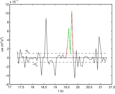
u′ >0 in the quadrant analysis plot, when using data acquired by Acoustic Doppler Velocimetry (ADV). Equations 2.5 and 2.6 show how these values are calculated and figure 2.5 shows graphically the threshold system used over the flow velocity fluctuation data.

σ+=2.5_×urms (2.5)

σ−=₋2.5_×urms (2.6)

It is commonly adopted that σh=σIh=σhII=σIIIh =σIVh and the domains that identify the occurrence of each event are described as:

• Outward interactions:Qout={u′,w′∈R:u′>0∧w′>σh_u′ ∧u′<σ+};

• Ejection interactions:Qe j={u′,w′∈R:u′<0∧ {w′>_|σh_u′_|∨u′<σ−}};

• Inward interactions:Qin={u′,w′∈R:u′<0∧w′<0∧ |w′|> _|σh_u′_|∧u′>σ−};

• Sweep interactions:Qsw={u′,w′∈R:u′>0∧ {{w′<0∧ |w′|>σh_u′} ∨u′>σ+}}.

Out Ej

In Sw

σ−

σ+ σ_h

(44)

(45)

Chapter 3

Particle Image Velocity

3.1 Principles

The Particle Image Velocimetry technique is based on the flow digital image processing and it is commonly addressed as non-intrusive because it is one of the less intrusive known techniques, as it only uses tracer particles in the stream. These tracers are illuminated by a pulsed light sheet in subsequent shots allowing to trace the stream turbulent structures.

In order to capture the tracing particles in a certain plane, the pulsed laser light is shaped into a thin light sheet by means of cylindrical and spherical lenses. While the tracer particles are being illuminated by the light sheet, they are captured by the camera, registering its positioning in two consecutive time instants.

This technique was incredibly improved in recent years, mainly due to the development of digital cameras and charge couple device technology, pulsed laser light and computer processing capabilities. Its main advantage is that it provides instantaneous velocity fields instead of punctual measurements or profiles in a single direction.

The method is mainly focused on the determination of displacement fields along a known time interval. This time interval must be short when compared to the minor time scales characteristics of the flow, in order to consider small displacements.

By knowing the particles displacement(∆di), and the time interval between two consecutive laser pulses(∆t), both components of instantaneous flow velocity are suitable to be calculated, as shown in equations 3.1 and 3.2.

u(x,z)_≃(x+∆dx)−x

∆t (3.1)

w(x,z)_≃(z+∆dz)−z

∆t (3.2)

The following Fig. 3.1 elucidates schematically how the method works.

(46)

Figure 3.1:PIV experimental setup. Adapted from Raffel et al. (1998).

It is of extreme importance to synchronize the camera with the laser beam, because they must be adjusted to a time interval adequate to the flow conditions. The camera may capture an image pair that occurs in a reduced time frame, so that the same set of particles is registered in both the images. This is possible to achieve recurring to a CCD high speed shutter camera, allowing the capture of images continuously and within a very short exposure time when compared to the time between two consecutive pulses(∆t). Fig. 3.2 represents schematically the synchronization of the laser beam with the CCD camera (Raffel et al., 1998).

Figure 3.2:Synchronization of the CCD camera with the laser pulses. From Lory (2011).

As represented in Fig. 3.2, the first laser pulse corresponds to the closing of the camera shutter and the next light beam corresponds to the opening of the camera shutter (Raffel et al., 1998). To help with this, there is a synchronization box in the laboratory, where both the CCD camera and the laser head are connected allowing to synchronize them by using a software in a personal computer.

The time interval between each frame pair is controlled by the user as it is input in the begin-ning of the experiments and kept constant during all procedure. If the first image frame is captured in the time instanttand the second image frame is captured in the time instantt, the time interval,

∆t, results from the 3.3.

t′=t+∆t (3.3)

(47)

Figure 3.3: A pair of images in the same frame position, results in an average displacement in an interro-gation area (Raffel et al., 1998).

An error is introduced when dividing the image frame in interrogation areas because this implies that the same particles are located inside the same interrogation area for both images of the same pair. This error grows with the increasing of the interrogation areas number inside the same image frame, which is the same as increasing the spatial resolution.

The Dynamic Studio software computes each interrogation area separately in correlation maps based in the correspondent image pair, interpreting the correlation function peak as being the average displacement vector of the correspondent interrogation area.

3.2 Correlation methods

A correlation method is a method of analysis based on a statistical approach that results in the most probable correspondence for each particle image pair between each captured pair of frames. Regarding each interrogation area, the correlation methods set that for a particle image in the first frame, all the particle images in the remaining frame are equally probable to be its pair, re-presenting a certain potential displacement. This is processed to all the particles and then these displacements are represented in a histogram. After setting this procedure for all particle images placed within the interrogation area, the effective displacement will be dominant over every other displacement.

To validate this procedure, there have to be two important requirements: The particle displa-cement inside each interrogation area have to be near uniform and each interrogation area have to contain a considerable number of particle images.

The Dynamic Studio software works with three different correlation methods,namely, the cross-correlation, the average-correlation and the adaptive-correlation, and the user must choose the most suitable method for the characteristics of the laboratorial experiments undertaken.

A correlation analyses results in a correlation plot such as the one in Fig. 3.4, where the coor-dinates of the peak correspond to the mean values of displacement in that interrogation area.

The cross correlation method is more often used as it improves the signal-to-noise ratio and eli-minates the ambiguity regarding flow direction (Westerweel, 1997; Raffel et al., 1998; Campbell, 2005).

(48)

Figure 3.4: Example of a correlation plot. The peak corresponds to the coordinates where the mean displacement estimation stands (Tropea et al., 2007).

These experiments were undertaken using the adaptive-correlation method, which results from improving the cross-correlation method by providing accuracy based on an adaptive interrogation area. This interrogation area is continuously decreased for a certain number of steps or until achieving a certain interrogation area previously introduced.

When achieving a first approach based on the simple cross-correlation method, the interrogation area becomes smaller and it is re-centred based on the highest peak.

This correlation method is particularly recommended in measurements where the flow velocity gradients are not negligible. However, the adaptive-correlation methods time consuming, around 3 times more than the simple cross-correlation method, under the same conditions (Simão et al., 2009).

Other methods are being developed in recent years, such as the adaptive central difference interrogation algorithm and adaptive forward difference algorithm. These methods allow maximi-zing the spatial resolution of the PIV technique.

The great advantage of using this technique, particularly the adaptive central difference interrogation algorithm, is because it improves accuracy as it produces better results when measuring flow near the boundaries and it produces results with higher signal-to-noise ratios, when compared to the simple cross-correlation (Wereley and Meinhart, 2000). These modified cross-correlation algorithms prove to be very helpful when high accuracy measurements are demanded.

3.3 Errors in PIV

In PIV measurements it is important to know and understand the possible error factors, in order to control them and minimize the spurious data as much as possible.

The most common limitations in PIV are related to camera damages, non-homogeneous laser light sheet, insufficient particles inside the interrogation areas or it can be limited by phenomena like:

(49)

The in-place loss of pairs occurs when tracer particles leave the interrogation area because they are a lot faster than the mean velocity within the image frame. This phenomenon con-tributes to lower the flow velocity estimation because the faster particles are not considered in the correlation function.

In order to prevent the in-plane loss of pairs there may be applied a sub-area in the borders of the interrogation area before performing the correlation method (Ferreira, 2011).

• Velocity gradients

The velocity gradients phenomenon is also a contribution to the in-plane loss of pairs and it happens when the velocity is not uniform inside the interrogation area. Therefore not all the tracer particles inside de interrogation area correlate equally well. This error becomes significant when the displacement of tracer particles due to local flow gradients becomes larger than the diameter of the particle (Tropea et al., 2007).

• Out-of-plane loss of pairs

This phenomenon results from particle movements in the camera axis, because tracer parti-cles may enter or leave the exposure sheet between the two pulses losing the correspondent pair. This results in a reduction of the signal-to-noise ratio and it is a PIV limitation that can be improved by simply adjusting the light sheet thickness (Tropea et al., 2007). Fig. 3.5 exemplifies the light sheet intensity profile where particles must stand to be captured by the camera. The light intensity is not constant in its whole thickness, which may result in particles less illuminated and therefore, with an inferior contrast in the captured image.

Figure 3.5:Laser sheet thickness (Raffel et al., 1998).

• Peak-locking

Peak-locking is mainly caused by improper sub-pixel estimation when the input data is dis-tributed asymmetrically around the maximum peak and therefore resulting in a displacement bias error (Tropea et al., 2007). It can be seen in Fig. 3.6 that there is not a clear peak, but the noise is dominating a possible true peak.

• Computational limitations

(50)

Figure 3.6: Example of a peak-locking phenomena in the correlation plot. The true peak is wrap-ped between noise (Ferreira et al., 2010).

The size of the interrogation area is of extreme importance because there have to be achieved a compromised between the accuracy and the spatial resolution. Using larger interrogation areas has the advantage of empowering the accuracy and it is very useful for larger motions but the large velocity gradients affect the results. On the other hand, choosing smaller interrogation areas improves the spatial resolution and it is less affected by the velocity gradients but raises inaccuracy and tracer particles must be smaller.

The choice of the interrogation area size depends on the characteristics of the flow and on the equipment available. However, a compromise must be achieved between the interrogation area size and the seeding quantity inserted in the flow, too.

In order to have a good particle density and homogeneity in the PIV images, Raffel et al. (1998) refers that in each interrogation area must be 12 seeding particles and its displacement may not be higher than 25% of the interrogation area side.

However, in the experiments previously performed at this laboratory with similar flow conditions, a number of 5 particles per interrogation area has been producing good results. It corresponds to around 56_{seeding particles per square meter of fluid.}

This is fundamental, regarding the choice of the interrogation area size. It means that when choosing a smaller interrogation area it is mandatory that the seeding quantity is increased also, in order to achieve the number of seeding particles needed per interrogation area.

3.4 Tracer particles

Choosing the right seeding or tracer particles is a factor of extreme importance to achieve reliable data. The seeding must represent precisely all flow motions because they are responsible for the achievement of punctual displacements by registering its successive position.

The tracer particles behaviour is mainly influenced by external forces, such as, gravity, centri-fugal and electrostatic, and by its own shape, diameter and specific mass. It is also influenced by the fluid characteristics, such as fluid density and dynamic viscosity.

Although the particle shape affects the flow resistance, it is neglected. All the particles are assumed to be spherical due to its small size, which is of around 10 to 80µm.

The contact between particles when suspended in the flow is neglected because under con-centrations around 109_particles_/_m3_{it is known that the distance between particles is around 1000}

(51)

According to Prasad (2000) there are two main conditions that tracer particles must satisfy in order to be used in PIV measurements. It has to follow the flow streamlines without slipping and they must be efficient light scatterers because if they are not, it must be compensated by improve-ments in the laser and camera technology which are very expensive.

The main condition for the particles to follow all flow fluctuations is the settling velocity under gravity in stagnant water. Assuming that the process is governed by Stokes drag, thus the settling velocity is given by equation 3.4.

Vsp=

g_×d2_p_×(ρp−ρf)

18_×µ (3.4)

whereVspstands for the settling velocity, grepresents the gravity acceleration,dp is the particle diameter,ρpandρf are the density of the particles and fluid, respectively and theµrepresents the fluid dynamic viscosity.

If theVspof a certain sort of particles is negligible when compared to the flow velocity, then it is warranted that these particles can represent perfectly all flow fluctuations.

Melling (1997) have also used a solution, based on Hjemfelt and Mockros (1996) results, to eva-luate the seeding particles ability to follow the flow without slipping. They applied the equation 3.5 to evaluate if the seeding is good enough to be used in PIV measurements.

V_p2

V2rp= (1+

2_×π_×fc 18_×µ )

−1 _(3.5)

where,ν, represents the kinetic fluid viscosity and fcis the frequency of turbulent structures. It relates the absolute particle velocity,Vpto the absolute flow velocity,V. Thus, ifρp=ρf then, Vp=V and the particles follow the fluid motion exactly, becauserp=1 (Chao, 1964). Melling (1997) stated that it is acceptable thatrpstand between 0.95 and 1.

Because it is difficult and considerably expensive to acquire particles with such characteristics, it is thus considered thatrp=0.95 represents a considerable significance. Andrpis then compared to the frequency of turbulent structures value, fc, achieving the relation represented in Fig. 3.7, which valid to the tracer particles used.